Sage Journals: Discover world-class research

Abstract

Issues with inflated false positive rates (FPRs) in brain imaging have recently received significant attention. However, to what extent FPRs present a problem for voxelwise analyses of Positron Emission Tomography (PET) data remains unknown. In this work, we evaluate the FPR using real PET data under group assignments that should yield no significant results after correcting for multiple comparisons. We used data from 159 healthy participants, imaged with the serotonin transporter ([¹¹C]DASB; N = 100) or the 5-HT₄ receptor ([¹¹C]SB207145; N = 59). Using this null data, we estimated the FPR by performing 1,000 group analyses with randomly assigned groups of either 10 or 20, for each tracer, and corrected for multiple comparisons using parametric Monte Carlo simulations (MCZ) or non-parametric permutation testing. Our analyses show that for group sizes of 10 or 20, the FPR for both tracers was 5-99% using MCZ, much higher than the expected 5%. This was caused by a heavier-than-Gaussian spatial autocorrelation, violating the parametric assumptions. Permutation correctly controlled the FPR in all cases. In conclusion, either a conservative cluster forming threshold and high smoothing levels, or a non-parametric correction for multiple comparisons should be performed in voxelwise analyses of brain PET data.

Keywords

Positron emission tomography false positives brain preprocessing multiple comparisons

Introduction

In recent years, there has been an increased focus on questioning the statistically significant findings in neuroimaging. The community has had a rising interest in the statistical validity of neuroimaging findings including general discussions regarding publication bias¹ and sample size.² There has even been a movement for redefining what statistical significance level should be used³ and a contra-movement arguing that a p-value threshold should be abandoned altogether.⁴ Most of these discussions are driven by theoretical considerations and general statistical arguments making them hard to follow for a general community.

But there have also been efforts to call attention to the effects of overestimating the statistical significance in real data. In spring of 2016, Eklund et al.⁵ showed that parametric-based clusterwise inferences have inflated false-positive rates (FPRs) in fMRI group analyses. In 2017, Greve and Fischl⁶ followed by highlighting the fact that surface-based anatomical analyses also have inflated FPRs. Furthermore, a few studies have addressed the FPRs in voxel-based morphometry (VBM),⁷ reporting elevated FPRs in the range of 10–50%, when using parametric clusterwise inferences.^8,9 Across these studies and across neuroimaging modalities, the authors have used real data and showed, using experiments mimicking common practices, how many false positive findings a regular analysis would yield. This has underscored the need for researchers to show more consideration of the underlying assumptions of their statistical models. These reports from fMRI, VBM and surface-based anatomical analyses also show that (non-parametric) permutation-based clusterwise inference properly controlled the FPR.

In the spirit of Eklund et al.⁵ and Greve and Fischl,⁶ we used a common analysis workflow for a voxelwise PET analysis^10,11 and investigated the FPR based on real PET data of 100 healthy controls scanned with the radioligand [¹¹C]DASB, targeting the serotonin transporter, and 59 healthy controls scanned with [¹¹C]SB207145, targeting the 5-HT₄ receptor. While the methodology is very similar to previous work in structural and functional MRI, the novelty of this work is in applying it to a new modality where the source of FPRs will be different and so the ability to control the FPRs with parametric methods uncertain.

PET analysis is most often performed on anatomically defined regions of interest (ROIs) in the brain. However, voxelwise analyses in PET neuroimaging are also prominent (see Table 1) as an exploratory technique to identify areas showing an effect when no a priori anatomical hypothesis exists.²² Voxelwise analyses have been applied in PET with varying preprocessing or statistical parameter choices (Table 1) such as sample size, motion correction (yes/no), spatial smoothing (6–12 mm), statistical analysis type (one-sided vs. two-sided group difference), and correction type for multiple spatial comparisons across voxels (multiple hypothesis testing). Currently, there exist no unified guidelines for carrying out voxelwise PET analyses, but in recent years the impact of preprocessing and statistical analyses on the final results have been investigated.^10,22,23 The application of motion correction has been shown to have a large impact on the results, as motion artefacts can invalidate the PET data.^10,24 However, while motion correction has been shown to be important, less attention has been given to the impact of smoothing levels, and the correction for multiple hypothesis testing. Typically, the spatial smoothing level and correction level for multiple testing are chosen with limited explicit knowledge of the exact impact on the results. Spatial smoothing is used to reduce noise and boost signal-to-noise ratio, and exploratory analyses have shown that it has a substantial effect.¹² In neuroimaging, correction for multiple testing has gained much attention due to work by Eklund et al.⁵ and Greve and Fischl.⁶ However, despite these alarming studies, several researchers still choose a cluster forming threshold (CFT) of p = 0.05, largely ignoring that this threshold will result in inflated false-positive rates.

Table 1.

Previous PET studies carrying out a voxelwise analysis.

Reference	N	MC	FWHM	Analysis type	Correction type
Matsumoto et al.¹²	18/4	No	12	One-sided test	CFT<0.001, 25v
Hesse et al.¹³	21/19	No	12	One-sided test	CFT<0.001, 30v
Lanzenberger et al.¹⁴	19	Yes	–	–	CFT<0.05, FDR
Hesse et al.¹⁵	22/23	No	12	One-sided test	CFT<0.005, 30v
Frick et al.¹⁶	18/18	Yes	12	–	CFT<0.005, FWE
Frick et al.¹⁷	18/18	Yes	8	Two-sided test	CFT<0.001, 640 mm³
Hesse et al.¹⁸	15/30	Yes	8	Two-sided test	CFT<0.005, 30v
McMahon et al.¹⁹	23	Yes	10	Two-sided test	Permutations
Deen et al.²⁰	16/15	Yes	6	Two-sided test	CFT<0.05, FWE
Hjort et al.²¹	43/27	Yes	12	One-sided test	CFT<0.05, FWE

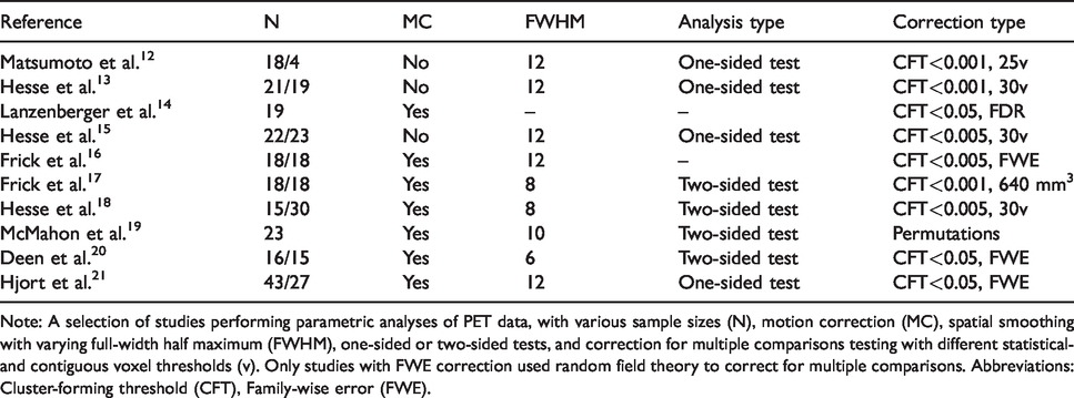
Note: A selection of studies performing parametric analyses of PET data, with various sample sizes (N), motion correction (MC), spatial smoothing with varying full-width half maximum (FWHM), one-sided or two-sided tests, and correction for multiple comparisons testing with different statistical- and contiguous voxel thresholds (v). Only studies with FWE correction used random field theory to correct for multiple comparisons. Abbreviations: Cluster-forming threshold (CFT), Family-wise error (FWE).

The aim of this paper is to evaluate the impact of voxelwise PET analyses and corrections for multiple testing on the FPR. We will investigate several aspects of voxelwise PET analyses ranging from preprocessing to correction for multiple comparisons and explore how these may have an impact on the FPR. This includes 1) the effect of different corrections for multiple statistical hypothesis tests, and 2) the effect of preprocessing choices, such as motion correction or spatial smoothing. Based on these results, we will provide guidelines that will adequately control the FPR. Furthermore, we will highlight which brain areas seem to be more sensitive to false positive results so that this information can be taken into account when interpreting and reporting results in future PET studies.

Methods

Dataset

The dataset used in this study is from the CIMBI database;²⁵ all data from this database are accessible upon request. A total of 159 unique PET scans and corresponding structural MRI scans were used to image either the serotonin transporter using the radioligand [¹¹C]DASB (N = 100) or the 5-HT₄ receptor using [¹¹C]SB207145 (N = 59).¹¹ Thirty of the available subjects also received a second [¹¹C]DASB scan, allowing for a longitudinal analysis. The acquisition of data was approved by the ethics committee for the capital region of Copenhagen. All subjects provided written informed consent prior to participation, in accordance with The Declaration of Helsinki II.

Acquisition and preprocessing

All PET and MR scans were analyzed in the individual’s volume space as described in Beliveau et al.¹¹ Briefly, the PET data was acquired on a Siemens High-Resolution Research Tomography (HRRT) PET scanner with a 90 and 120 minutes scan for [¹¹C]DASB and [¹¹C]SB207145, respectively (matrix size = 256 × 256 × 207; voxel size = 1.2 mm). PET data was reconstructed using a 3 D-OSEM-PSF^26–28 with a point spread function (PSF) of 4 mm and was corrected for head motion using AIR (v. 5.2.5). The MRI data was acquired as an isotropic T1-weigthed MP-RAGE for all participants (matrix size = 256 × 256 × 192; voxel size = 1 mm; TR/TE/TI = 1550/3.04/800 ms; flip angle = 9°) using either a Siemens Magnetom Trio 3 T or a Siemens 3 T Verio MR scanner. All MR data was processed using FreeSurfer v.5.3²⁹ (but no surface-based analysis was used). For each subject, the PET data was co-registered to the MRI data using a boundary-based registration (BBR),³⁰ and subsequently spatially normalized with an affine transform to a 2 × 2 × 2 mm standard space using the MNI305 atlas provided by FreeSurfer (matrix size: 76 × 76 × 93). The total size of the mask covering the brain was 304,611 voxels. All group analyses were carried out in MNI305 space. The PET data was smoothed with 4, 6, 8, 10 or 12 mm full width half maximum (FWHM) using a 3 D Gaussian kernel, and the non-displaceable binding potential (BP_ND) was then quantified for each voxel in PETsurfer,²² based on dynamic PET acquisitions and kinetic modeling with MRTM2 with cerebellum (excluding vermis) as reference region.³¹ This results in voxelwise maps of BP_ND for each subject and at each smoothing level. For the longitudinal data, the data were additionally processed either with/without motion correction, or with 0 or 6 mm spatial smoothing using a 3 D Gaussian kernel. Longitudinal data allows us to evaluate the impact of possible subject-specific neuroreceptor features (similar to the effect of unique anatomical features as found in Greve and Fischl⁶).

Random group analyses

Following Eklund et al.⁵ and Greve and Fischl,⁶ for each of the two radioligands, 20 (or 40) subjects were randomly selected, and randomly assigned to one of two groups of size 10 (or 20). The motivation for choosing these group sizes is that they reflect common sample sizes of clinical PET studies. A two-group two-sided voxelwise GLM analysis was performed on the BP_ND maps for each of the five selected spatial smoothing levels. As no covariates (e.g. age or sex) were added in the GLM analysis, the model simply corresponds to a t-test of independent group means. Clusters were formed by thresholding the voxel-wise maps at cluster forming thresholds (CFT) of 0.05, 0.01 and 0.001. Since we assume that there are no actual group differences, any significant cluster (p < 0.05) is interpreted as a false positive outcome. The analysis was repeated 1,000 times and the resulting fraction of false positives represented our estimate of the FPR (Figure S1). The FPR is expected to be 50/1,000 = 5% false positives. P-values for clusters were estimated using permutations and Monte Carlo (MCZ) simulations, as implemented in FreeSurfer.²⁹ MCZ simulations are simply volumes of simulated Gaussian noise smoothed with a Gaussian kernel at a FWHM equal to that found in the residuals of the group analysis; the volume is thresholded at the CFT and the maximum cluster size recorded and used to estimate the null distribution of the cluster size in real data. Conclusions that apply to MCZ will also apply to random field theory (see Greve and Fischl⁶ for more details). In total, we performed 120,000 group analyses (see Table 2). For MCZ, look up tables of cluster p-values were created for thresholds of CFT<.05, .01, .001 over a FWHM range of 1–30 mm of smoothing levels measured in the data. The probability of a cluster at a given size can therefore be computed for a given smoothness level, by indexing it into the look up table. One of the main parametric assumptions in the MCZ method is that the smoothness of the data follows a Gaussian distribution, determined by the estimated global FWHM. The global FWHM was computed using the correlation coefficient between the residuals of the GLM analysis between neighboring voxels (first lag of a spatial autoregressive model), and then averaged over all voxels. The residuals were estimated from the GLM by subtracting the fitted data from the actual data. The full spatial autocorrelation function (ACF) can be computed by estimating the correlation between the residuals at different spatial distances. Skewness was estimated from the residuals at each voxel.

Table 2.

Parameter choices.

Parameter	Values used
PET data	[¹¹C]DASB (100 subjects), [¹¹C]SB207145 (59 subjects)
Smoothing	4, 6, 8, 10 or 12 mm FWHM
Analysis type	Two-sample t-test (group difference)
No. of subjects	20, 40
Correction type	Permutations, Gaussian-based Monte Carlo Simulation (MCZ)
CFT	p = 0.05 (z = 1.96), p = 0.01 (z = 2.3), p = 0.001 (z = 3.1)

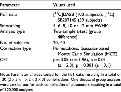
Note: Parameter choices tested for the PET data, resulting in a total of 120 (2 × 5 × 1 × 2 × 2 × 3) combinations. One thousand group analyses were carried out for each combination of parameters resulting in a total of 120,000 analyses.

For permutations, the design matrix was permuted, followed by the recomputation of significance maps, thresholding, and extraction of the cluster with maximal size.³² This was repeated 1,000 times to generate a null distribution of maximal cluster sizes. The empirical p-value for a given cluster was then computed as the probability of seeing a cluster larger than the observed size in the permuted null distribution. Confidence intervals (CI) for the estimated FPR were computed using a binomial model with 5% frequency and 1,000 trials.⁶ All code used to generate the results presented in this paper can be found on GitHub (github.com/Neurobiology-Research-Unit/PET_FPR). In addition, the reporting of the experimental setup used in this work is in accordance with the guidelines for the content and format of PET brain data.³³

Results

Figure 1 shows the empirical FPRs for [¹¹C]DASB and [¹¹C]SB207145 group analyses, corrected for multiple comparisons using MCZ and permutations. For MCZ, the FPRs are highly inflated for both radioligands, both displaying an interaction between the CFT and smoothing level. Only a CFT = 0.001 and a FWHM of 12 mm result in an expected range of 5% FPR. For permutations, only a CFT = 0.05 and a FWHM of 4 mm result in marginally inflated FPRs. The remaining settings behaved with little dependency on CFT and FWHM, with all combinations falling within the nominal 95% confidence interval of the expected FPR. Notably, the dependencies between FPR, FWHM and smoothing level were comparable between the two tracers.

Figure 1.

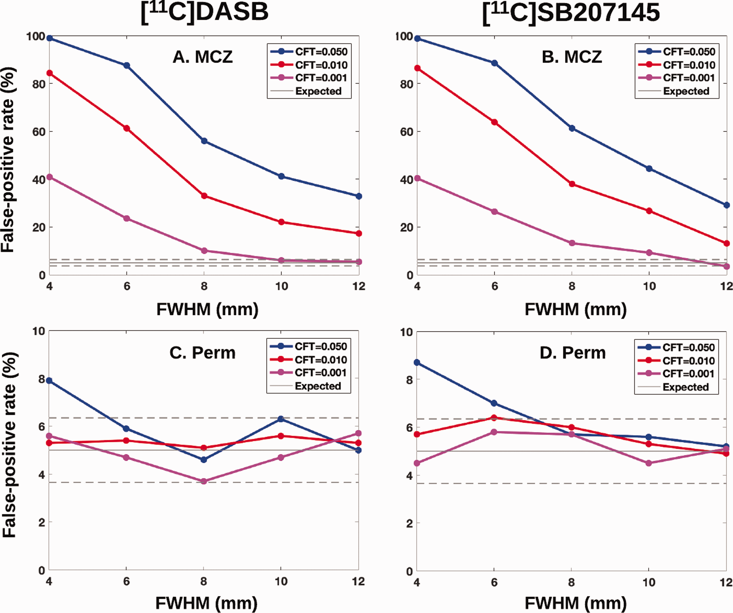
Clusterwise false positive rates (%) versus applied smoothing level for the two radioligands [¹¹C]DASB and [¹¹C]SB207145 (10/group) and for either parametric Monte Carlo simulations (A-B, MCZ) or permutations (C-D, Perm). Dashed lines are the 95% significance level. Abbreviations: Full-Width Half Maximum (FWHM).

Extent of false-positive clusters

The cluster extent thresholds to obtain significance at CFT = 0.05 were 3-4 times higher for permutation correction than MCZ (Table 3 and S1). For example, for [¹¹C]DASB with 8 mm smoothing a significant mean cluster size was 6,766 voxels (CI: 1,947;34,415) using MCZ and p < 0.05, whereas a mean cluster size using permutations was 37,968 voxels (CI: 18,155; 69,887). According to Figure 1, permutation correction and MCZ correction became very similar at high CFT and high smoothing levels, whereas the high FPR for low smoothing levels and low CFT were largely driven by small clusters.

Table 3.

Cluster sizes for significant cluster at different cluster forming thresholds.

	p < 0.05	p < 0.01	p < 0.001
4 mm	942 (275;4,340)	203 (86;713)	62 (30;202)
4 mm	13,737 (5,202;33,994)	1,245 (695;3,110)	184 (107;422)
6 mm	2,761 (778;16,087)	593 (235;2,055)	159 (80;482)
6 mm	26,743 (11,868;54,719)	3,129 (1,410;10,850)	372 (215;422)
8 mm	6,766 (1,947;34,415)	1,518 (574;6,865)	420 (205;1,579)
8 mm	37,968 (18,155;69,887)	5,708 (2,125;21,075)	659 (313;2,094)
10 mm	13,528 (3,755;56,476)	3,448 (1,168;16,179)	1,041 (380;3,618)
10 mm	45,038 (24,401;108,680)	10,081 (3,408;41,540)	1,267 (425;4,164)
12 mm	19,064 (5,953;69,090)	5,583 (1,984;38,693)	1,778 (645;10,226)
12 mm	55,820 (29,807;113,165)	13,153 (4,203;55,126)	1,708 (557;9,808)

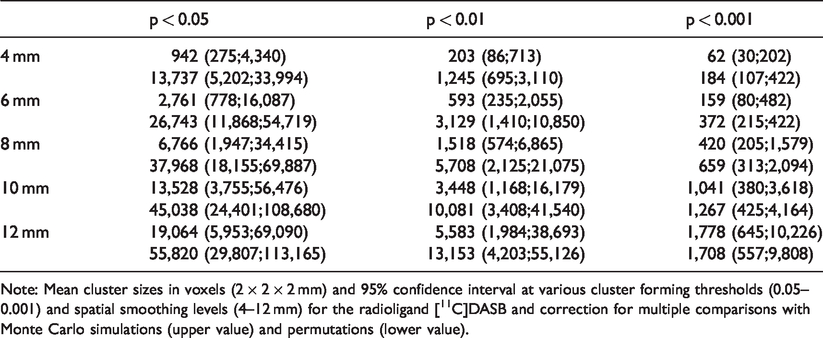
Note: Mean cluster sizes in voxels (2 × 2 × 2 mm) and 95% confidence interval at various cluster forming thresholds (0.05–0.001) and spatial smoothing levels (4–12 mm) for the radioligand [¹¹C]DASB and correction for multiple comparisons with Monte Carlo simulations (upper value) and permutations (lower value).

Spatial distribution of false-positives clusters

To investigate whether the spatial distribution of false-positive clusters was randomly distributed throughout the brain, all significant clusters were binarized and summed together to create a frequency map of clusters. The frequency map in Figure 2 for [¹¹C]DASB (10/group) reflects the brain areas that are more likely to be significant in a voxelwise analysis using clusterwise parametric correction. The insula, temporal and anterior cingulate cortices were the most likely areas to contain a cluster, whereas white matter, cerebellum and the brainstem were least likely. These local hot spots are likely to reflect higher than average local smoothness, violating the main parametric assumption of stationary smoothing across the entire brain. Notably, the effect was found to be radioligand-specific, with [¹¹C]SB207145 displaying a completely different spatial distribution of false-positive clusters with increased FPRs in the hippocampus, amygdala, ventricles, orbitofrontal cortex, and parietal and occipital cortices (Figure S2). This suggests that the non-stationary smoothing is not necessarily a scanner artefact, but rather interacts with the radioligand to affect the spatial smoothness.

Figure 2.

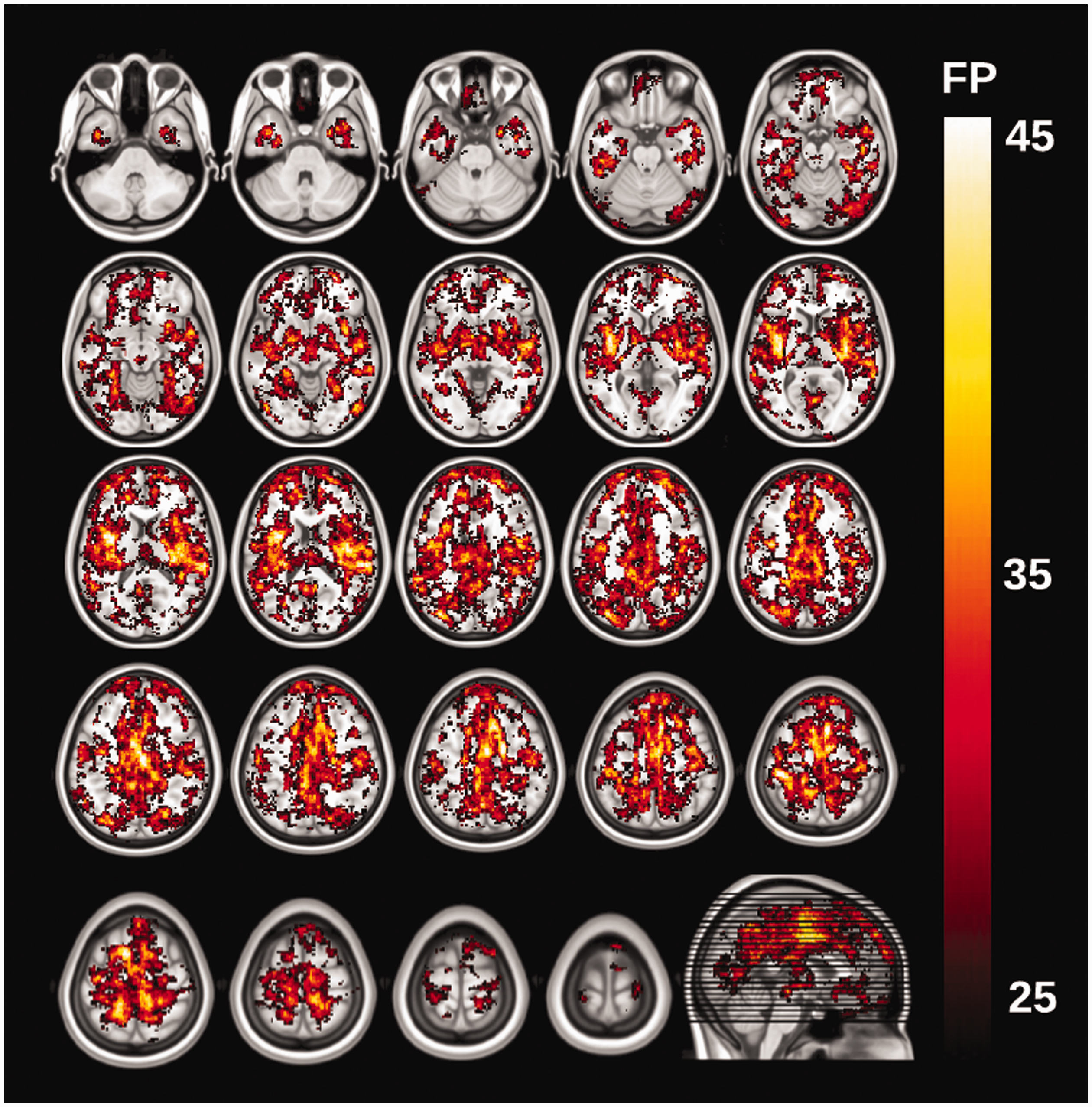
The maps show the spatial distribution of false-positive clusters. The image intensity of the overlay (red/yellow) is the number of instances (false positives, FP), out of 1,000 random group analyses for [¹¹C]DASB (10/group, 8 mm smoothing), a significant cluster occurred at a given voxel (CFT = 0.05, p < 0.05).

Spatial autocorrelation function of the noise

The behavior of the spatial ACF, averaged over all brain voxels, was investigated for distances of 1–30 mm and for spatial smoothing levels of 4–12 mm FWHM. The empirical ACFs are given in Figure 3, including a reference squared exponential based on the computed global FWHM. The empirical ACFs are far from following a squared exponential, having much heavier tails. Consistently with Eklund et al.⁵ and Greve and Fischl,⁶ this explains why the parametric methods work well for a high CFT and not as well for a low CFT, reflecting local and distant autocorrelation, respectively.

Figure 3.

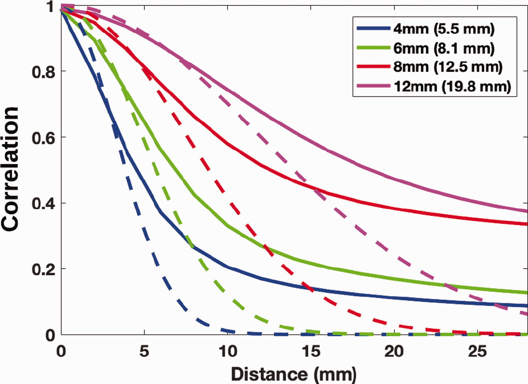
Spatial autocorrelation function (SACFs) for the [11C]DASB data (10/group) for nominal smoothing levels of 4, 6, 8 and 12 mm. The values in the parentheses are the estimated FWHM of the residuals. The dashed lines are the theoretical Gaussian ACF computed using the estimated FWHM. All SACFs are heavy-tailed compared to the Gaussian ACF.

Longitudinal analysis and preprocessing

To understand the origin of the heavy tails, the spatial autocorrelation function was estimated with various combinations of preprocessing (after motion correction and spatial smoothing) using the longitudinal dataset (Figure 4). The residuals from the longitudinal data set were estimated by subtracting the mean difference over the 30 subjects at each voxel from each of the 30 BP_ND estimates. The ACFs were then estimated from the paired difference residuals.⁶ The longitudinal dataset was used to investigate the possibility of anatomical features unique to individuals being the explanation for the heavy tails.⁶ Consistently with Eklund et al.,⁵ we observed that the heavy tails exist in the raw data. The longitudinal analysis slightly decreased the size of the tails compared to the cross-sectional analysis but was still far from the theoretical squared exponential. Overall, because the heavy tails seem to be present in the data without preprocessing, this suggests that the heavy tails originate from the PET acquisition and/or reconstruction and are amplified during the various preprocessing steps.

Figure 4.

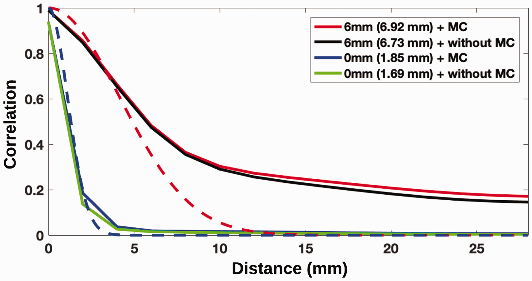
Spatial autocorrelation function (SACFs) for raw PET data (no MC and smoothing), PET data after smoothing, and PET data after motion correction. A theoretical squared exponential is displayed as a reference (dotted line) at smoothing level 0 mm (blue) and level 6 mm (red). The SACFs were estimated using the longitudinal DASB dataset (N = 30). Abbreviations: Motion Correction (MC).

Skewness

There was no consistent pattern of skewness in either the cross-sectional or longitudinal data examined (skewness ranging between -0.19 and 0.16), suggesting that the data are symmetrical and normally distributed.

Discussion

In this study, we tested whether parametrically computed clusterwise p-values are valid in voxelwise group analyses of PET BP_ND data by empirically measuring the FPRs. Across different radioligands, the FPRs were largely inflated up to 99% for CFT’s larger than 0.001 and smoothing levels below 12 mm. This is worse than for structural MRI⁶ and functional MRI⁵ at matching CFT and smoothing levels. These results were consistent across different tracers, group sizes (Figure S3), longitudinal and cross-sectional analyses, and for different preprocessing choices. Similar to structural MRI⁶ and fMRI,⁵ the FPRs were well-controlled at 5% by using high CFT and high smoothing levels or by using non-parametric permutation correction instead of a parametric correction. While we focused on controlling the FPR at the cluster level, a post hoc analysis at the voxel level using parametric correction showed conservative FPRs, consistent with previous observations⁵ (Figure S5).

Like fMRI and structural MRI, the source of the problem was found to be spatial ACFs whose tail was heavier than the Gaussian assumed by the parametric correction. Looking at the residual for two subjects from the cross-sectional group analysis (Figure S4A-B), one can see that there are large patches where the residuals are either positive or negative (indicating that the BP_ND is above or below the group mean). The same effect was found in structural data.⁶ These large patches are an indication of long-range spatial correlations in the BP_ND within subject that are not captured well by a Gaussian kernel. Unlike structural data, the spatial pattern of these patches appears to change over time within subject (as indicated by the longitudinal analysis, Figure S4C) and hence this probably does not represent an underlying subject-specific pattern of neuroreceptor density; this also suggests that a longitudinal analysis would not be spared from inflated FPRs.

The source of these patches is most likely due to the nature of the acquisition and analysis. The PET acquisition is dynamic with multiple time points. The quantification of PET data is based on dynamic data acquisitions where the time-activity data are modeled based on a reference region, meaning that brain regions are likely to be correlated with each other as in resting state fMRI³⁴; use of an arterial input function (AIF), instead of a reference region TAC, may result in lower spatial correlation due to it being independent of the imaging data.

This is now the fourth neuroimaging modality to demonstrate elevated FPRs caused by heavy-tailed ACFs, the other three being fMRI, VBM MRI, and surface-based morphometry (SBM) MRI. Given the results in these other modalities, it might not be surprising to find them in PET. However, each modality will have its own unique source of long-range spatial correlation, so each modality needs to be evaluated separately. For example, the heavy-tailed ACFs disappeared in longitudinal SBM but are still present in longitudinal PET, and different PET tracers had a different spatial distribution of false clusters.

Impact of inflated false-positive rates

Focusing specifically on the inflated FPRs, it is important to be aware of the implications of our results. As previously mentioned, it is common to perform PET voxelwise analysis in an exploratory fashion. On the one hand this is reassuring, since, in PET, biological findings are more often based on ROI, not voxelwise, analyses. But in practice, inflated FPRs will lead to false signals in exploratory analyses which, in turn, can lead to the false selection of a priori regions for future analyses. This should be considered carefully when screening the literature for support of scientific hypotheses previously to designing new studies. In addition, this should be especially considered when performing human studies involving PET, since PET is more costly and invasive than other neuroimaging techniques, such as structural or functional MRI. We point out that our results apply to clusterwise p-values near the .05 level; if previous studies had clusters that were nominally more significant, then they might still be significant at the .05 level even after proper correction.

Effects of the spatial distribution of false-positive clusters

The spatial distribution of false-positive clusters was found to be distinct between the two radioligands, with region-specific non-stationary smoothing, affecting the local frequency of false positives. The most likely regions to contain a cluster were found to be areas with high radioligand uptake in combination with high susceptibility to partial volume effects. This included the putamen-insula region for [¹¹C]DASB, and the ventricles for [¹¹C]SB207145. While meta-analyses and comparisons between different studies can often help to tease apart true biological from false findings for generating new biological hypotheses, it is problematic if the FPRs are higher for certain areas in the brain, such as high-binding areas, because those areas will be repeatedly falsely activated and result in false positives in a meta-analysis. Therefore, it is crucial not to be misled by spurious findings in exploratory analyses when designing new biological hypotheses and to use accurate statistical tools that give valid results for each and every study.

Effects of radioligand

While [¹¹C]DASB and [¹¹C]SB207145 had similar overall FPRs, the distribution of false clusters was wildly different. For [¹¹C]DASB, the cluster frequency map showed evidence of hot spots in the insula and anterior cingulate cortex, suggesting that these areas have high smoothness. We speculate that this high smoothness might be caused by nearby high-binding regions (putamen and caudate) and partial volume effects. For [¹¹C]SB207145, the main hot spot was the ventricles. Notably, the high FPR in the ventricles was only present in the CFT = 0.05 threshold but was removed for CFT = 0.01. In a post-hoc analysis, we identified that all voxels in the ventricles had BP_ND below 0, suggesting that a proper threshold and/or better definition of a whole brain mask will limit the degree of false positives. For example, Deen et al. 2018, using [¹¹C]SB207145 and a threshold of BP_ND > 0.3 to create a brain mask a priori to any statistical analysis, obtained no significant clusters despite a parametric correction for multiple comparisons using a CFT = 0.05. It is of note though, that it is not standard procedure to threshold BP_ND values in voxelwise analysis, but this should be considered.

However, for both radioligands, the uptake in high-binding regions is slow and shows lower identifiability of the BP_ND, and a high variability in the estimate between subjects.³⁵ Consequently, the higher variability in BP_ND between subjects in the high-binding regions compared to low and/or medium binding regions, may make the spatial smoothness vary across the brain, leading to a higher degree of FPRs. Notably, it has been shown for VBM data that local smoothness systematically varies with tissue type, with frontal and temporal areas displaying a high degree of false positives.⁸ For resting-state fMRI, Eklund et al.⁵ identified the posterior cingulate, part of the default mode network (DMN), as a local hot spot with high smoothness, arguing that non-stationarity is a possible contributing factor. The DMN will be constantly activated in resting-state fMRI, similarly to high signal in high-binding regions for dynamic PET, and we speculate that the non-stationary smoothness is the primary cause of the spatial distribution of FPRs.

Effects of preprocessing and kinetic modeling

The degree of smoothing had a major effect on the ACF (Figure 3). While we smoothed the voxelwise time activity curves (TACs) before kinetic modeling, it is possible to smooth the BP_ND maps after kinetic modeling, and this may have an effect on the correlation and the FPRs. In the vast majority of studies, smoothing is carried out before performing kinetic modeling because the noise at the voxel level is high and will consequently lead to an unstable solution of the model fit (Greve et al.⁶). However, there are also examples in the literature applying spatial smoothing after kinetic modeling (e.g. Frick et al.¹⁶). To investigate the effect further, we carried out a post hoc analysis using the first time point of the longitudinal data set. Specifically, we applied a 6 mm filter either before or after kinetic modeling using MRTM2 and estimated the corresponding ACFs (Figure S6). The ACF with smoothing after kinetic modeling was markedly lower compared to the ACF with smoothing applied before, approaching the theoretical ACF. However, when inspecting the residual variance maps of the group analysis (Figure S7), the variance when smoothing after kinetic modeling was dramatically higher than smoothing before. This suggests that the noisy estimates from kinetic modeling and subsequent smoothing breaks the spatial correlation structure in the BP_ND maps and produces a lower ACF. While this is positive in the sense that the corresponding FPR will be lower, it comes at the expense of higher variance and inaccurate estimates at the subject-level, potentially producing spurious results in a group analysis.

Various kinetic modeling approaches have also been used in voxelwise analyses of PET data such as MRTM2¹⁴ and Logan Graphical analyses.¹⁶ These kinetic models do not have the same variance properties²⁴ and may result in different ACFs and consequently affect the FPR. To investigate this further, we also analyzed the first time point of the longitudinal data with 6 mm smoothing and Logan graphical analysis³⁸ and compared the ACF between MRTM2 and Logan (Figure S8). The ACF for Logan was similar but slightly more heavy-tailed than MRTM2. When inspecting the residual variance maps of the group analysis (Figure S9), we found that Logan produced lower between-subject variance compared to MRTM2, in line with previous work.²⁴ These results suggest that kinetic models with varying variance properties will have an impact on the FPRs but that elevated FPRs in parametric clusterwise analysis will remain.

Feasibility of using non-parametric testing

Based on our data, we strongly recommend that in the future, voxelwise PET analyses should adapt more stringent multiple comparison correction and higher smoothing levels. We advocate for the use of non-parametric methods for multiple comparison correction. While previously the computational complexity was the main drawback of permutation tests, this is not an issue with the recent increase in computational power. Also, we would like to point out that although permutation tests in voxelwise analyses have only rarely been used in PET, all major neuroimaging packages (SPM, FSL, FreeSurfer, PALM) and their extensions offer the possibility of calculating empirical cluster p-values via permutations. Hence, the statistical tools are also freely available. The presence of non-stationarity can cause the p-values to be too conservative in less smooth regions, but it is possible to account for this by modifying the computation of the cluster size to incorporate local smoothness information.³⁶ While permutation tools are readily available and easy to apply, it is not always possible to apply them correctly because the data must be exchangeable. Exchangeability means that the joint distribution of the data is invariant under permutation. This can be violated when PET data are skewed. Eklund et al.⁵ reported skewness in the fMRI one-sample t-tests, where the aim is to compare a sample mean to a hypothesized population mean, and that this skewness caused the permutation correction to be inaccurate; they found no skewness in the two-sample t-tests, where they compare the means of two samples. We found no significant skewness in our two-sample tests. While skewness should always be tested, our results suggest that skewness is not a barrier to perform proper permutation tests in PET. Exchangeability can also be violated by the presence of systematic effects across subjects (e.g., age effects), though approximations exist for the latter violation.³⁷ While permutations can be difficult to apply correctly, the tradeoffs in using permutations seem worthwhile in the face of such inflated FPRs with parametric methods.

Conclusions

We found that voxelwise analyses of PET data using parametric clusterwise correction for multiple comparisons can result in highly inflated FPRs up to 99%, much higher than for structural and functional MRI. The FPR at various smoothing levels and CFTs is independent of the tracer, but the spatial location of the false positives depends on the tracer. The FPRs were properly controlled by using non-parametric permutation.

Supplemental Material

sj-pdf-1-jcb-10.1177_0271678X20974961 - Supplemental material for False positive rates in positron emission tomography (PET) voxelwise analyses

Supplemental material, sj-pdf-1-jcb-10.1177_0271678X20974961 for False positive rates in positron emission tomography (PET) voxelwise analyses by Melanie Ganz, Martin Nørgaard, Vincent Beliveau, Claus Svarer, Gitte M Knudsen and Douglas N Greve in Journal of Cerebral Blood Flow & Metabolism

Footnotes

Funding

The author(s) disclosed receipt of the following financial support for the research, authorship, and/or publication of this article: Dr. Ganz’s work was supported by the Lundbeck (R181-2014-3586) and Elsass (18-3-0147) foundations. Dr. Norgaard was supported by funding from the Independent Research Fund Denmark (0129-00004B). Dr. Greve was supported by funding from the US National Institutes of Health grants U24DA041123, R01NS083534, R01EB023281, R01NS105820, R01NS112161.

Acknowledgements

We wish to thank all the participants for kindly joining the research project. We thank the John and Birthe Meyer Foundation for the donation of the cyclotron and PET scanner. Finally, we thank the anonymous reviewers for their comments that helped improve this paper.

Declaration of conflicting interests

The author(s) declared no potential conflicts of interest with respect to the research, authorship, and/or publication of this article.

Authors’ contributions

GMK acquired the data. MN, MG, DNG, GMK, CS, VB analyzed the data. MN, MG and DNG drafted the manuscript, and MG, MN, VB, CS, GMK and DNG revised and contributed to the final version.

ORCID iDs

Melanie Ganz

Martin Nørgaard

Claus Svarer

Supplementary material

Supplementary material for this article is available online.

References

Ioannidis

JPA.

Why most published research findings are false. PLoS Med 2005; 2: e124.

Button

Ioannidis

JPA

Mokrysz

, et al. Power failure: why small sample size undermines the reliability of neuroscience. Nat Rev Neurosci 2013; 14: 365–376.

Benjamin

Berger

Johannesson

, et al. Redefine statistical significance. Nat Hum Behav 2018; 2: 6–10.

McShane

Gal

Gelman

, et al. Abandon statistical significance. Am Stat 2019; 73: 235–245.

Eklund

Nichols

Knutsson

Cluster failure: why fMRI inferences for spatial extent have inflated false-positive rates. Proc Natl Acad Sci 2016; 113: 7900–7905.

Greve

Fischl

False positive rates in surface-based anatomical analysis. NeuroImage 2018; 171: 6–14.

Ashburner

Friston

KJ.

Voxel-based morphometry the methods. NeuroImage 2000; 11: 805–821.

Silver

Montana

Nichols

TE.

False positives in neuroimaging genetics using voxel-based morphometry data. NeuroImage 2011; 54: 992–1000.

Scarpazza

Nichols

Seramondi

, et al. When the single matters more than the group (ii): addressing the problem of high false positive rates in single case voxel based morphometry using non-parametric statistics. Front Neurosci 2016; 10: 6.

10.

Nørgaard

Ganz

Svarer

, et al. Cerebral serotonin transporter measurements with [11C]DASB: A review on acquisition and preprocessing across 21 PET centres. J Cereb Blood Flow Metab 2019; 39: 210--222

11.

Beliveau

Ganz

Feng

, et al. A high-resolution in vivo atlas of the human brain’s serotonin system. J Neurosci 2017; 37: 120–128.

12.

Matsumoto

Ichise

Ito

, et al. Reduced serotonin transporter binding in the insular cortex in patients with obsessive-compulsive disorder: a [11C]DASB PET study. NeuroImage 2010; 49: 121–126.

13.

Hesse

Stengler

Regenthal

, et al. The serotonin transporter availability in untreated early-onset and late-onset patients with obsessive-compulsive disorder. Int J Neuropsychopharmacol 2011; 14: 606–617.

14.

Lanzenberger

Kranz

Haeusler

, et al. Prediction of SSRI treatment response in major depression based on serotonin transporter interplay between median raphe nucleus and projection areas. NeuroImage 2012; 63: 874–881.

15.

Hesse

van de Giessen

Zientek

, et al. Association of central serotonin transporter availability and body mass index in healthy Europeans. Eur Neuropsychopharmacol 2014; 24: 1240–1247.

16.

Frick

Ahs

Engman

, et al. Serotonin Synthesis and Reuptake in Social Anxiety Disorder: A Positron Emission Tomography Study. JAMA Psychiatry 2015; 72: 794--802.

17.

Frick

Ahs

Palmquist

, et al. Overlapping expression of serotonin transporters and neurokinin-1 receptors in posttraumatic stress disorder: a multi-tracer PET study. Mol Psychiatry 2015; 21: 1400–1408.

18.

Hesse

Rullmann

Luthardt

, et al. Central serotonin transporter availability in highly obese individuals compared with non-obese controls: a [11C] DASB positron emission tomography study. Eur J Nucl Med Mol Imaging 2016; 43: 1096–1104.

19.

McMahon

Nørgaard

Svarer

, et al. Seasonality- resilient individuals downregulate their cerebral 5-HT transporter binding in winter: a longitudinal combined 11C-DASB and 11C-SB207145 PET study. Eur Neuropsychopharmacol 2018; 28: 1151–1160.

20.

Deen

Hansen

Hougaard

, et al. High brain serotonin levels in migraine between attacks: a 5-HT4 receptor binding PET study. NeuroImage Clin 2018; 18: 97–102.

21.

Hjorth

Frick

Gingnell

, et al. Expression and co-expression of serotonin and dopamine transporters in social anxiety disorder: a multitracer positron emission tomography study. Mol Psychiatry. Epub ahead of print 10 December 2019. DOI: 10.1038/s41380-019-0618-7.cs

22.

Greve

Svarer

Fisher

, et al. Cortical surface-based analysis reduces bias and variance in kinetic modeling of brain PET data. NeuroImage 2014; 92C: 225–236.

23.

Greve

Salat

Bowen

, et al. Different partial volume correction methods lead to different conclusions: an 18F-FDG-PET study of aging. NeuroImage 2016; 132: 334–343.

24.

Nørgaard

Ganz

Svarer

, et al. Optimization of preprocessing strategies in positron emission tomography (PET) neuroimaging: a [11C]DASB PET study. NeuroImage 2019; 199: 466–479.

25.

Knudsen GM, Jensen PS, Erritzoe D, et al. The Center for Integrated Molecular Brain Imaging (Cimbi) database. Neuroimage 2016; 124: 1213--1219.

26.

Comtat C, Sureau FC, Sibomana M, et al. Image based resolution modeling for the HRRT OSEM reconstructions software. In: 2008 IEEE Nuclear Science Symposium Conference Record, Dresden, Germany, 2008, pp. 4120--4123.

27.

Hong

Chung

Kim

, et al. Ultra-fast symmetry and SIMD-based projection-backprojection (SSP) algorithm for 3-D PET image reconstruction. IEEE Trans Med Imaging 2007; 26: 789–803.

28.

Sureau

Reader

Comtat

, et al. Impact of image-space resolution modeling for studies with the high-resolution research tomograph. J Nucl Med 2008; 49: 1000–1008.

29.

Fischl

FreeSurfer. NeuroImage 2012; 62: 774–781.

30.

Greve

Fischl

Accurate and robust brain image alignment using boundary-based registration. NeuroImage 2009; 48: 63–72.

31.

Ichise

Liow

J-S

J-Q

, et al. Linearized reference tissue parametric imaging methods: application to [11C]DASB positron emission tomography studies of the serotonin transporter in human brain. J Cereb Blood Flow Metab 2003; 23: 1096–1112.

32.

Nichols

Holmes

AP.

Nonparametric permutation tests for functional neuroimaging: a primer with examples. Hum Brain Mapp 2002; 15: 1–25.

33.

Knudsen

Ganz

Appelhoff

, et al. Guidelines for the content and format of PET brain data in publications and archives: A consensus paper. J Cereb Blood Flow Metab 2020; 40: 1576--1585.

34.

Biswal

Zerrin Yetkin

Haughton

, et al. Functional connectivity in the motor cortex of resting human brain using echo-planar MRI. Magn Reson Med 1995; 34: 537–541.

35.

Ogden

Ojha

Erlandsson

, et al. In vivo quantification of serotonin transporters using [(11)C]DASB and positron emission tomography in humans: modeling considerations. J Cereb Blood Flow Metab 2007; 27: 205–217.

36.

Hayasaka

Phan

Liberzon

, et al. Nonstationary cluster-size inference with random field and permutation methods. NeuroImage 2004; 22: 676–687.

37.

Winkler

Ridgway

Webster

, et al. Permutation inference for the general linear model. NeuroImage 2014; 92: 381–397.

38.

Logan

Fowler

Volkow

, et al. Distribution volume ratios without blood sampling from graphical analysis of PET data. J Cereb Blood Flow Metab 1996; 16: 834–840.

Supplementary Material

Please find the following supplemental material available below.

For Open Access articles published under a Creative Commons License, all supplemental material carries the same license as the article it is associated with.

For non-Open Access articles published, all supplemental material carries a non-exclusive license, and permission requests for re-use of supplemental material or any part of supplemental material shall be sent directly to the copyright owner as specified in the copyright notice associated with the article.

0.00 MB

1.24 MB