Sage Journals: Discover world-class research

Abstract

The functional connectivity of the default-mode network (DMN) monitored by functional magnetic resonance imaging (fMRI) in Alzheimer's disease (AD) patients has been found weaker than that in healthy participants. Since breathing and heart beating can cause fluctuations in the fMRI signal, these physiological activities may affect the fMRI data differently between AD patients and healthy participants. We collected resting-state fMRI data from AD patients and age-matched healthy participants. With concurrent cardiac and respiratory recordings, we estimated both physiological responses phase-locked and non-phase-locked to heart beating and breathing. We found that the cardiac and respiratory physiological responses in AD patients were 3.00 ± 0.51 s and 3.96 ± 0.52 s later (both p < 0.0001) than those in healthy participants, respectively. After correcting the physiological noise in the resting-state fMRI data by population-specific physiological response functions, the DMN estimated by seed-correlation was more localized to the seed region. The DMN difference between AD patients and healthy controls became insignificant after suppressing physiological noise. Our results indicate the importance of controlling physiological noise in the resting-state fMRI analysis to obtain clinically related characterizations in AD.

Keywords

Respiratory response function cardiac response function resting-state classification physiological noise fMRI network

Introduction

Different from identifying active brain areas by examining the correspondence between the regional waveform and the modeled responses informed by the experimental paradigm in task-related fMRI,¹ resting-state fMRI studies how hemodynamics at brain areas are correlated to each other in the resting condition, where participants do not explicitly engage in specific tasks and/or stimuli processing.² Since the first study demonstrating such a correlation between bi-hemispheric sensorimotor areas, the topology of the resting-state network has been reported extensively (for review, see Cole et al.³ and Rosazza and Minati⁴). One resting-state network includes the posterior cingulate cortex (PCC), medial prefrontal cortex (mPFC), hippocampus, and lateral parietal lobes.⁵ During a broad range of cognitive processing, these areas are routinely exhibiting task-related deactivations.⁶ Thus, this resting-state network has been named as the “default mode” network (DMN) because it supports the default activity of the human brain.^7–9

Compared with healthy participants, Alzheimer’s disease (AD) patients have significantly decreased activity at the DMN.^10–15 The spatial topology of the DMN revealed in these studies matches the distribution of the amyloid-beta (Aβ) plaque deposition.¹⁶ The spatial association suggests the neurochemical basis of the DMN and the application of using DMN as an imaging marker to distinguish between AD patients and healthy participants.

The noise in DMN affects the sensitivity and specificity of DMN characterization. One dominant noise source in the blood-oxygen-level-dependent (BOLD)-contrast fMRI signal, particularly at the MRI field strength higher than 3 T, is the physiological noise,^17,18 the fluctuation in fMRI time series caused by physiological processes unrelated to the experimental manipulation. Physiological noise ultimately limits the time-domain signal-to-noise ratio (tSNR) to be obtained at high MRI field strength,¹⁹ because the noise amplitude scales with the signal strength.¹⁷ Studies have suggested the importance of suppressing the physiological noise from cardiac pulses and respiration in order to delineate the DMN with higher specificity by avoiding the inflated estimate of the strength of the functional connectivity and the spatial extent of the DMN.¹⁷ In addition to cardiac and respiratory cycles, other physiological processes, such as heart beat-to-beat variability and the variation on the respiration volume across respiratory cycles, can also cause BOLD signal fluctuations.²⁰ Previous studies found that AD patients have altered vascular structures^21,22 and blood flow regulation.²³ The hemodynamic response is known to be affected by cardiac and respiratory cycles, which are likely to be different between AD patients and healthy participants.^24,25 Therefore, it is possible that the differences found in previous papers can be attributed to such differences but not the underlying neuronal processes. These sources of noise should be correctly estimated in order to provide more accurate functional connectivity characterization.

In this study, we investigated how physiological fluctuations affect the DMN in AD patients using BOLD fMRI. In particular, we compared the DMN in AD patients with healthy age-matched participants. Previous studies showed that the DMN in AD patients is less active than healthy participants.^10–14 Here we tested two hypotheses. First, the vascular responses to cardiac and respiratory cycles are different between AD patients and healthy participants because the vascular responses and neurovascular coupling have been pathophysiologically altered in AD patients.²⁶ Second, without controlling the physiological noise using the population-specific physiological response function, the difference in DMN between AD patients and healthy participants can be erroneously inflated. The novelty of our study is thus to provide quantitative models for physiological response functions for AD and age-matched healthy participants and to quantify the difference in the functional connectivity between healthy and AD cohorts after physiological noise suppression.

Methods

Demographics

Fifteen patients with AD (9 females; 77.9 ± 5.9 years) and 17 age-matched healthy participants (10 females; 77.4 ± 7.2 years) were recruited in the experiment. The number of participated patients and healthy participants matched that in a previously published study.¹³ The age of the healthy subjects did not differ significantly from those of the AD group (t = 0.18, p = 0.85). No significant difference in the educational background between both participant groups. This study was approved by the Institutional Review Board at National Taiwan University Hospital. All participants provided written informed consent before the experiment. This study followed the guidelines in the Declaration of Helsinki.

MRI data acquisition

All MR scanning was performed on a 3 T MRI scanner (Magnetom Tim Trio, Siemens, Erlangen, Germany) with a 32-channel head coil array. Brain structural images were acquired using a T₁-weighted pulse sequence (MPRAGE; TR = 2530 ms, TE = 3.03 ms, FOV = 256 mm, flip angle = 7^°, matrix size = 224 × 256, voxel size = 1 × 1×1 mm³, GRAPPA acceleration = 2).

Resting-state fMRI scans used a T₂*-weighted echo-planar imaging (EPI) sequence. Imaging parameters were: TR = 2 s, TE = 30 ms, FOV = 220 mm, flip angle = 90°, matrix size = 64 × 64, slice thickness = 3.5 mm; total acquisition = 400 s. All participants were instructed to keep their eyes closed and not engage in any particular thought. They were also instructed to stay awake, alert, and not to move their bodies as best as they can.

Physiological signal monitoring

Cardiac and respiratory cycles were measured by a photoplethysmograph placed on the index fingertip and a respiration belt strapped around the upper abdomen (Siemens, Erlangen, Germany) for each participant, respectively. Cardiac and respiratory cycle waveforms, as well as the onset of each EPI volume, were recorded. The sampling rate of measuring cardiac and respiration cycles was 50 Hz.

Data analysis

Preprocessing of fMRI data included: intra-session 3D motion correction, slice timing correction, co-registration between fMRI and anatomical data, spatial normalization to the MNI space, and spatial smoothing. The spatial smoothing used an isotropic Gaussian kernel of 5-mm full-width-half-maximum. These pre-processing steps were done by Statistical Parametric Mapping (SPM8, Wellcome Department, University College London, UK; http://www.fil.ion.ucl.ac.uk/spm/software/spm8/) and the Resting State fMRI Data Analysis Toolkit (REST 1.8, State Key Laboratory of Cognitive Neuroscience and Learning, Beijing Normal University; http://restfmri.net/forum/REST_V1) implemented in Matlab (version R2014a, MathWorks, Sherborn, MA, USA).

The BOLD signals included temporal confounds not related to physiological noise. In this study, confounds included motion (three translation terms and three rotation terms), average white matter (WM) signal, average cerebrospinal fluid (CSF) signal, a constant and a linear term to describe temporal drift. Six motion-related terms were estimated by image realignment using SPM8. Average WM and CSF signals were extracted by the REST toolbox. These covariates were included in the design matrix as regressors to model confounds in all analyses.²⁷

Physiological response function estimation

We separately estimated both the respiratory response function (RRF)²⁸ and cardiac response function (CRF)²⁰ for healthy participants and AD patients. The estimation started from calculating the “respiratory variations (RV)” time series, which was the standard deviation of the respiratory cycle waveform within a 6-s window,²⁹ and heart rate (HR) time series, which was the inverse of the beat-to-beat interval between two cardiac pulses smoothed over a 6-s window²⁹ for each participant. RV and HR were first normalized to Z-scores by subtracting the mean of the RV (or HR) and then dividing by the standard deviation of the mean-removed RV (or HR) time series.

We took an iterative process to estimate brain areas that were significantly affected by RV and HR and their response functions (RRF and CRF). The algorithm of this iterative estimation is described below.

The estimation of RRF and CRF waveforms started by identifying the image voxels, where their fMRI time series were significantly affected by RRF and CRF. These locations were initially estimated by using previously published RRF and CRF models.^20,28 Once these regions were revealed, their time series were concatenated to obtain the first RRF and CRF estimates using the CVX package. This procedure suggested by a previous study²⁹ prevented us from being biased toward any specific RRF or CRF model.

Estimate brain areas affected by RV/HR:

1.1 RV was first convolved with the RRF, and HR was convolved with the CRF. These two convoluted time series were then used as regressors in a general linear model (GLM) to identify brain areas where the fMRI time series had significant (FDR corrected p < 0.001) regression coefficients. In this GLM, two temporal confounds (constant and linear terms) were added to the design matrix.

Estimate the response function

2.1The ROI was identified as the intersection of brain areas with significant regression coefficients with RV convolved with RRF and with HR convolved with CRF. Times-series data of these ROI areas were first averaged across voxels and then concatenated across participants.

2.2Another GLM was performed on the concatenated average time series. The design matrix of this GLM consisted of the RV convolved with RRF waveform and its 1st and 2nd-order temporal derivative as well as the HR convolved with CRF waveform and its 1st and 2nd-order temporal derivative.

2.3The estimated response function was updated by a linear combination of the 0th, 1st, and 2nd-order temporal derivative of the currently estimated response function. The coefficients for the linear combination were estimated coefficients of corresponding terms.

2.4Go to step 1.1.

This iterative estimation was repeated multiple times to ensure convergence. Supplementary Figure 1 illustrates this process. To ensure the convergence of the calculation, we compared how the estimated response function varied between iterations by calculating the sum of squares of the difference (SSD) between two consecutive response function estimates. When the estimated response function did not change significantly between iterations, we considered that we had a converged estimate of the response function.

Upon reaching convergence in RRF and CRF estimation, a GLM was performed to estimate their latencies with respect to the previously published RRF²⁸ and CRF²⁹ models. Specifically, the 0th and 1st-order temporal derivatives of the model were used as regressors to fit the iteratively estimated RRF and CRF. The latency was taken as the ratio between the 1st and the 0th-order coefficients.³⁰ This latency estimate was based on Taylor’s expansion: the response function with the unknown latency was best approximated by the sum of the 0th-order response model weighted by the 0th-order coefficient and the 1st-order response model with the latency to be estimated. Thus, the ratio between the coefficients for the 1st and the 0th-order term provided the latency estimate. Direct estimating the peak timing of the response function is error-prone because the sampling rate was too coarse (with TR = 2 s). In other words, we cannot differentiate timing differences confidently if it is within 2 s.

To further estimate the variability of population-specific RRF and CRF estimates and their latencies, we used the bootstrap method to repetitively estimate RRF and CRF and their latencies by resampling participants within each group with replacement 100 times. For the visualization purpose, estimated physiological response functions for AD patients and healthy participants were normalized by dividing the physiological response waveform to their maximal values.

Physiological noise suppression

Physiological noise suppression included two steps. First, the RETROICOR method³¹ was applied after spatial normalization and before slice timing³² to remove time-locked artifacts related to cardiac rhythms and respiratory cycles. The RETROICOR was implemented by in-house codes. Specifically, by simultaneously recording the respiration cycles and heartbeats during the fMRI acquisition, we first convert the cardiac rhythm and breathing time series into phases (between 0 and 2π). Then, low-order Fourier series were fit to the image data based on time of each image acquisition relative to the phase of the cardiac and respiratory cycle.³¹ The fitted sinusoidal oscillation was subsequently removed from the original time series. Non-time locked physiological noise (fluctuations not depending on the phase of the cardiac/respiratory activity) was estimated by the RVHRCOR method²⁰ to remove effects related to the respiration volume (RV) and heart rate variability (HR). Specifically, the RV waveform was convolved with the estimated RRF to generate the expected BOLD response of the RV time series. Similarly, the HR waveform was convolved with the estimated CRF, which was either the previously published CRF²⁰ or our group-specific estimate, to generate the expected BOLD response of the HR time series. The RV and HR covariates were included in the design matrix together with the motion, temporal drift, WM, and CSF time series as regressors to model confounds.²⁷ For comparison, we also calculated results after RVHRCOR with previously published RRF and CRF. This approach was described as “standard RVHRCOR” in order to contrast the RVHRCOR with group-specific RRF and CRF.

It is possible that adding more regressors to suppress the physiological noise may reduce the degree of freedom and over-fit the fMRI time series. To address this concern, in a separate analysis, we randomly shuffled the estimated RRF and CRF to generate two artificial response functions. Then, the shuffled RRF and CRF were convolved with RV and HR, respectively, as two additional regressors in the design matrix. This analysis was denoted as “RF-shuffled RVHRCOR” to reveal the effect of the different degrees of freedom in the analysis.

Image quality analysis

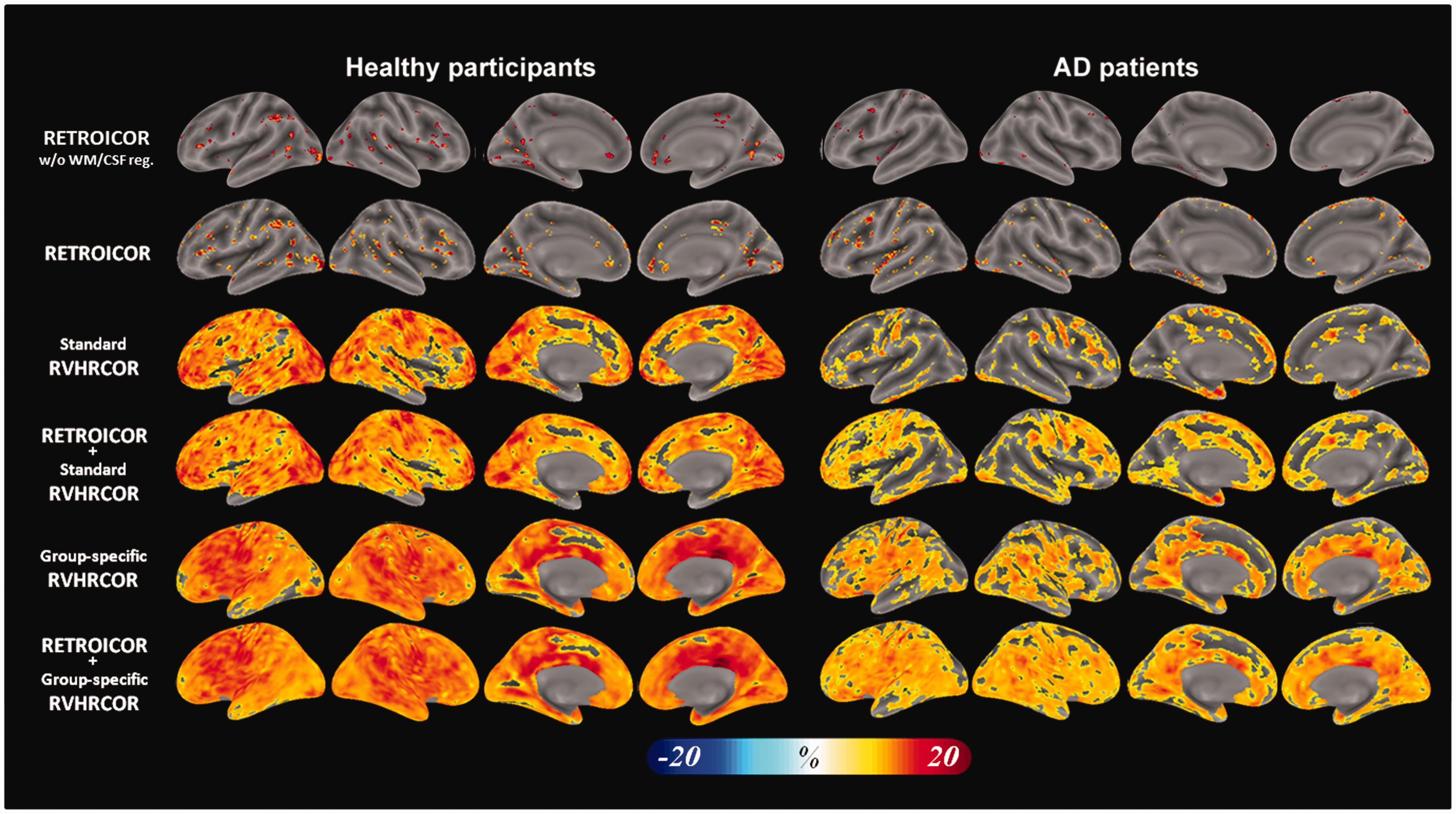
We assessed the image quality by calculating the time-domain signal-to-noise ratio (tSNR) maps. The temporal drift modeled by a constant and a linear trend term was first removed from the fMRI time series by regression. Labeling the average signal intensity as s and its standard deviation over time as $σ$ , the tSNR at a specific location in the brain was calculated

tSNR = \frac{S}{σ}

(1)

A paired t-test was applied to each voxel in the tSNR maps to test whether the tSNR was improved after RETROICOR and/or RVHRCOR. The tSNR difference (before and after physiological noise suppression) maps between healthy participants and AD patients were also compared. Statistical tests were corrected for multiple comparisons by controlling the false discovery rate (FDR) q = 0.05 to avoid errors related to multiple comparisons in these calculations.

Resting-state functional connectivity analysis

Functional connectivity was estimated by the seed-based correlation method.³³ A band-pass filter with cutting-off frequencies of 0.01 Hz and 0.08 Hz was used to filter the fMRI time series before the functional connectivity analysis.² Then, we calculated correlation maps with seeds at the PCC (Brodmann Area 10) and mPFC (Brodmann Area 31), respectively. Each seed region was defined by a 5-mm diameter sphere centered at previously published MNI coordinates: PCC [0, −53, 26] and mPFC [0, 52, −6].^34,35

Correlation coefficients maps were transformed to Z-score maps. These DMN’s with or without physiological noise suppression in AD patients or healthy participants were then compared. We were specifically interested in two contrasts: (i) between healthy participants and AD patients, and (ii) with and without physiological noise suppression. Statistical tests were corrected for multiple comparisons by controlling the false discovery rate (FDR) q = 0.05 to avoid errors related to multiple comparisons in these calculations.

Results

Motion analysis

The head motion was not significantly different between the two groups of participants (translation: healthy participants = 0.44 ± 0.27 mm, AD = 0.50 ± 0.28 mm, t = 0.62, p = 0.54; rotation: healthy participants = 0.68 ± 0.45°, AD = 0.65 ± 0.38°, t = 0.20, p = 0.84).

Physiological response functions

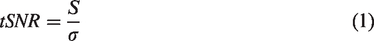
Figure 1(a) shows the RRF and CRF estimated from healthy participants, AD patients, and previously published models.^28,29 The amplitudes of the estimated CRF and RRF were scaled, such that their maximal values were 1. The variation shown with each RRF and CRF was derived from bootstrap samples. We found 20 iterations gave convergent estimates of RRF and CRF (Supplementary Figure 2) in both participant groups. The estimated RRF latencies for the healthy participants and AD patients were 1.23 ± 0.38 s earlier and 2.73 ± 0.37 s later than the previous RRF model,²⁸ respectively. The estimated CRF latencies for the healthy participants and AD patients were 0.33 ± 0.34 s earlier and 2.67 ± 0.38 s later than the previous CRF model,²⁹ respectively. We found that AD patients have more delayed RRF (3.96 ± 0.52 s, t = 27.87, p < 0.0001) and CRF (3.00 ± 0.51 s, t = 29.06, p < 0.0001) than healthy participants. We found that the CRF may appear similar between the group-specific estimate (in this study) and the one derived from young healthy participants,²⁹ their waveforms still differed between each other in the widths of post-stimulus over-shoot and under-shoot. Figure 1(b) and (c) shows the areas whose BOLD signal has significant regression coefficients with the RV/HR using the convolution of RV/HR and group-specific RRF/CRF or previously published RRF/CRF (standard RVHRCOR). We found that, in healthy participants, the regions significantly affected by RV cover almost the entire brain. In contrast, regions significantly affected by HR were more focused, primarily in the occipital cortex, PCC, and lateral prefrontal cortex. Comparing healthy participants with AD patients, we found that physiological noise caused by RV and HR was stronger in healthy participants than in AD patients. Specifically, physiological components related to RV were found to be stronger in healthy participants in the occipital cortex, middle temporal cortex, medial prefrontal cortex (mPFC), and PCC. On the other hand, physiological components related to HR were found to be stronger in healthy participants in the occipital cortex.

Figure 1.

Group-specific physiological response functions and brain areas sensitive to physiological response functions. (a) Respiratory response function (RRF) and cardiac response function (CRF) estimated from AD patients (red), healthy participants (blue), and previously published data (green). (b) Spatial distributions of Z-scores characterizing the significance of the correlation between local fMRI time series and RV convolved with previously published RRF (left) or HR convolved with previously published CRF (right) in healthy controls (top row), AD patients (middle row). The difference in the significance of this correlation between population groups is shown in the bottom row. (c) Spatial distributions of Z-scores characterizing the significance of the correlation between local fMRI time series and RV convolved with group-specific RRF (left) or HR convolved with group-specific CRF (right) in healthy controls (top row), AD patients (middle row). The difference in the significance of this correlation between population groups is shown in the bottom row.

fMRI time-series analysis

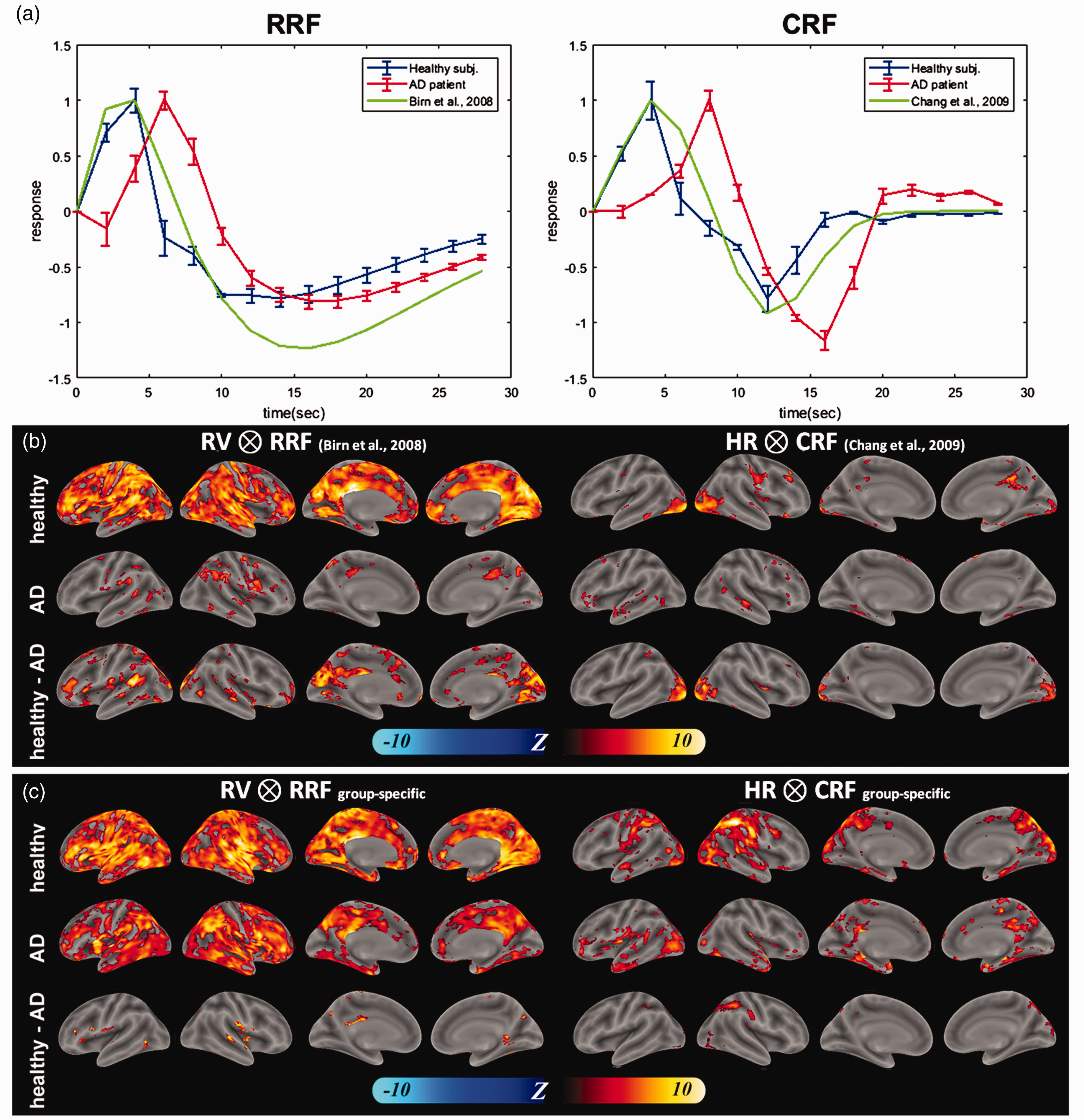
Here we quantified how physiological noise suppression affected the tSNR of the fMRI time series. Figure 2 shows the mean and standard deviation of the tSNR in AD patients and healthy participants over the whole brain and over gray matter. Significant tSNR improvement was found after RETROICOR and/or RVHRCOR. Applying both RETROICOR and RVHRCOR provided the largest tSNR improvement and caused larger differences between subject groups than applying either method alone. Data after RVHRCOR using group-specific response functions had significantly higher tSNR than data after RVHRCOR using previously published response functions (standard RVHRCOR).²⁰

Figure 2.

Physiological noise suppression improves tSNR, which differs between healthy participants and AD patients at gray matter (left) and whole brain (right). The bar height and the vertical black bar represent the average and the standard deviation of the tSNR, respectively. Physiological noise suppression significantly improves the tSNR across the whole brain (left) and at gray matter (right). Data were (1) without physiological noise suppression (“uncorrected”; yellow), with RETROICOR only (orange), with group-specific RVHRCOR only (red), with both RETROICOR and group-specific RVHRCOR (blue), and with both RETROICOR and standard RVHRCOR (cyan). The largest improvement was found using both group-specific RETROICOR and RVHRCOR. Single and double asterisks represent the statistically significant difference with the threshold of p = 0.05 and p = 0.01, respectively (uncorrected for multiple comparison).

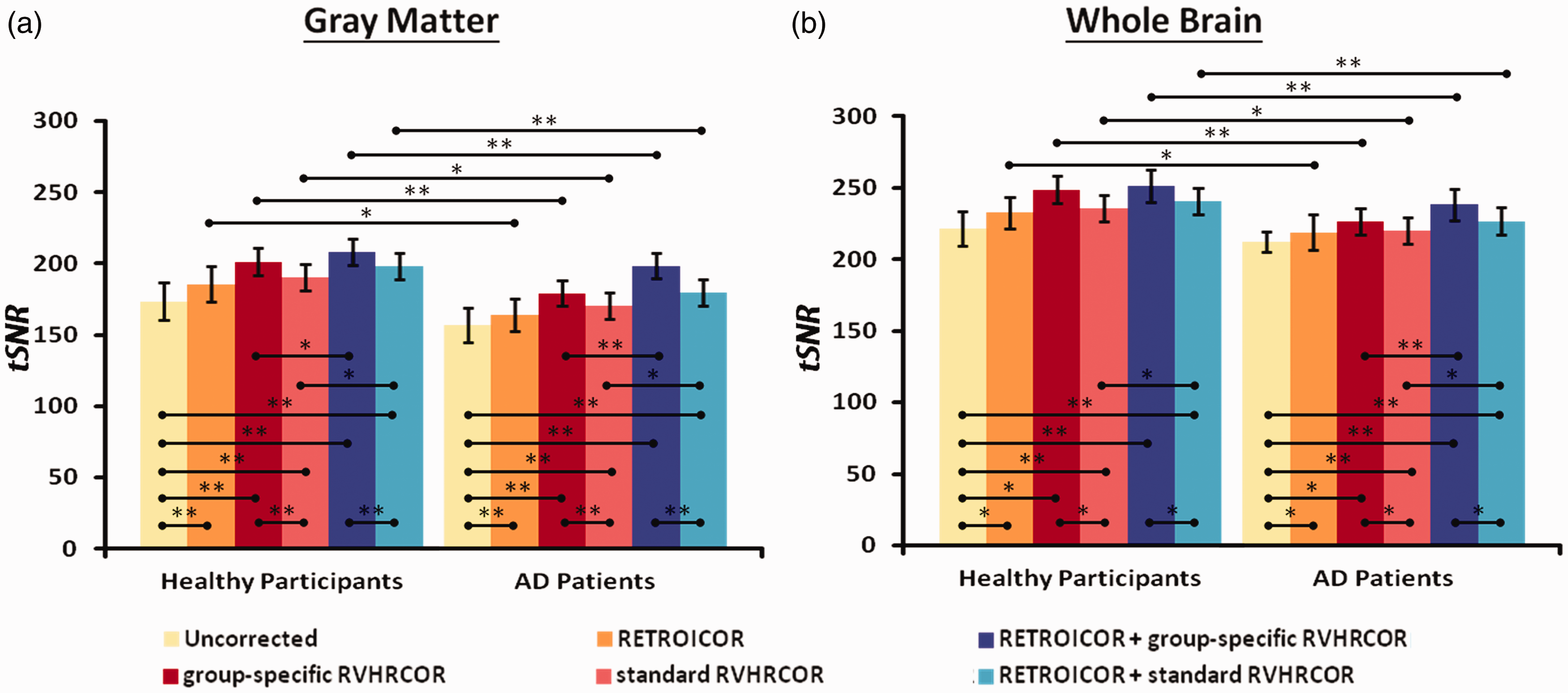
Figure 3 shows tSNR difference maps using fMRI data before and after physiological noise suppression. These maps were separately calculated for healthy participants and AD patients. The regions with significant tSNR improvement by RETROICOR were sparsely distributed. RETROICOR improved the tSNR at scattered locations at the cortex (the top row in Figure 3). The regression using the time series from WM and CSF after RETROICOR only marginally improved the tSNR (the 2nd row in Figure 3). Group-specific RVHRCOR, on the other hand, contributed to significant tSNR improvement almost over the entire brain (the 3rd row in Figure 3). The improvement was stronger – covering even more voxels in healthy participants than in AD patients. Applying both RETROICOR and group-specific RVHRCOR provided the largest tSNR improvement than applying either method alone (the 4th row in Figure 3). Group-specific RVHRCOR caused more tSNR improvement than standard RVHRCOR, particularly for AD patients (the 5th and bottom rows in Figure 3). Figure 3 did not show a sharp transition between corrections using RVHRCOR and RETROICOR as Figure 2. This was likely due to the fact that we also presented the uncorrected baseline condition in Figure 3.

Figure 3.

The distribution of significant tSNR improvement by different physiological noise suppression methods in healthy participants (left) and AD patients (right). The top row shows the results without WM and CSF regression. All other rows show the results with WM and CSF regression. Physiological noise suppression used RETROICOR (the 1st and the 2nd rows) caused spatially scattered tSNR improvement. Standard RVHRCOR (the 3rd and 4th rows) improved the tSNR across the whole cortex. The largest tSNR improvement was found after both RETROICOR and group-specific RVHRCOR (the bottom row).

Figure 4 shows the comparison between healthy participants and AD patients in the tSNR difference map before and after physiological noise suppression. We found that (1) the tSNR improvement by RETROICOR did not differ much between groups; (2) The tSNR improvement by group-specific RVHRCOR was more in healthy participants than AD patients in the lateral prefrontal cortex, temporal cortex, and cingulate cortex; (3) Applying both RETROICOR and group-specific RVHRCOR, we observed higher tSNR improvement at similar areas as in (2); 4) Applying both RETROICOR and standard RVHRCOR caused higher tSNR across the whole brain in healthy participants than in AD patients. This is likely due to the relative minor tSNR improvement by standard RVHRCOR in AD patients (Figure 4).

Figure 4.

The difference in the distribution of significant tSNR improvement by different physiological noise suppression methods between healthy participants and AD patients. These maps were comparison between left and right columns of Figure 5. Physiological noise suppression used RETROICOR (top row), group-specific RVHRCOR (the 2nd row), the combination of RETROICOR and group-specific RVHRCOR (the 3rd row), and the combination of RETROICOR and standard RVHRCOR (bottom row). Significance level: p < 0.001 after controlling the false discovery rate.

Functional connectivity analysis

DMN characterization

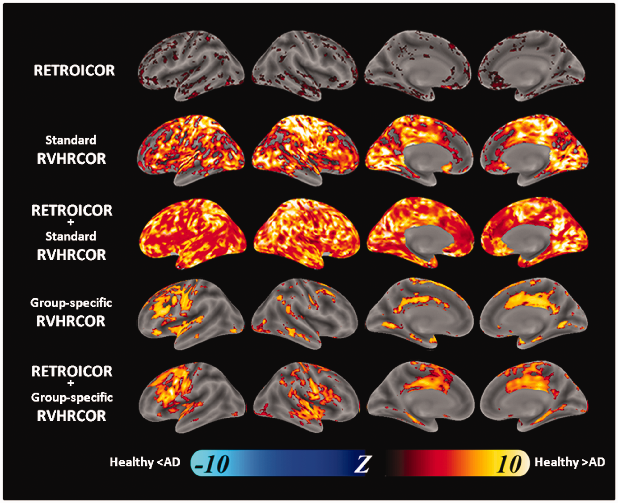
Figure 5 shows significant DMN maps. Using PCC as the seed region (Figure 5(a)), we found that its functional connectivity with mPFC was reduced after physiological noise suppression. Specifically, RETROICOR marginally reduced the extent of the DMN, while group-specific RVHRCOR caused much reduced DMN. Bi-hemispheric middle temporal gyri were estimated to be a part of DMN in the healthy participants. However, they were no longer considered to be functionally connected to PCC after group-specific RVHRCOR. The functional connectivity between PCC and the bi-hemispheric sensorimotor cortices in both groups became insignificant after group-specific RVHRCOR. Similarly, taking mPFC as the seed region (Figure 5(b)), we found that the functional connectivity at PCC was mostly reduced after physiological correction. This difference was larger after group-specific RVHRCOR than after RETROICOR. For example, the functional connectivity between mPFC and anterior temporal lobes became insignificant after group-specific RVHRCOR. As for the comparison between standard RVHRCOR and group-specific RVHRCOR, data after group-specific RVHRCOR had more focal DMN than data after standard RVHRCOR. The effect of physiological noise suppression using shuffled RRF and CRF was minimal compared with the uncorrected results.

Figure 5.

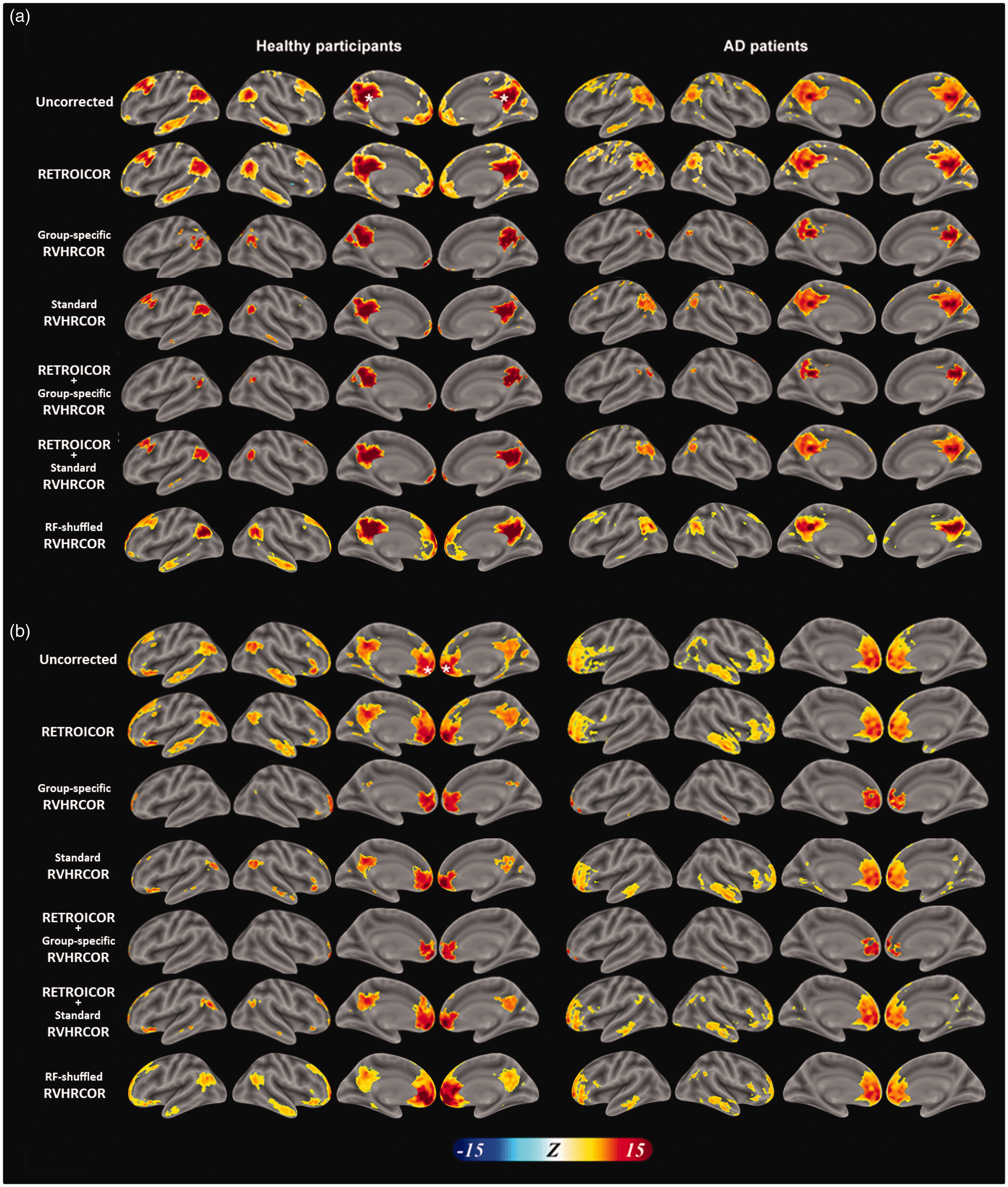
DMN maps before and after physiological noise suppression. DMN maps in healthy participants (left) and AD patients (right) derived from time series with the seeds at posterior cingulate cortex (PCC; a) and medial pre-frontal cortex (mPFC; b) with different combinations of physiological noise suppression. Different rows represent DMN estimated from the uncorrected time series, time series after RETROICOR, time series after group-specific RVHRCOR, time series after the combination of RETROICOR and group-specific RVHRCOR, or time series after the combination of RETROICOR and standard RVHRCOR. White asterisks denote the location of the seed regions.

Comparing DMN’s between AD patients and healthy participants

We further compared the DMN difference (before and after physiological noise) between AD patients and healthy participants (Figure 6). It depicts how physiological noise suppression affects the functional connectivity difference between groups. Taking PCC as the seed region, we found that AD patients showed a larger DMN difference than healthy subjects in mPFC, inferior parietal lobule (IPL), and right inferior temporal cortex. While this difference was still significant after RETROICOR, it was not significant in IPL and right inferior temporal cortex using group-specific RVHRCOR. The DMN difference in mPFC was still significant but with a much-reduced size even after applying both RETROICOR and group-specific RVHRCOR. Similarly, taking mPFC as the seed region (Figure 6(b)), the DMN difference in healthy participants was found to be larger than that of AD patients in PCC and IPL. Again, the DMN difference between groups was insignificant in PCC. This difference became much reduced in IPL after suppressing physiological noise using both RETROICOR and group-specific RVHRCOR. Overall, applying group-specific RVHRCOR made the DMN difference between AD and healthy participants less distinct than applying RETROICOR. This reduction in DMN difference was even more prominent when two approaches were jointly used than either method alone. The same finding was found in standard RVHRCOR. The effect of physiological noise suppression using shuffled RRF and CRF was minimal compared with the uncorrected results.

Figure 6.

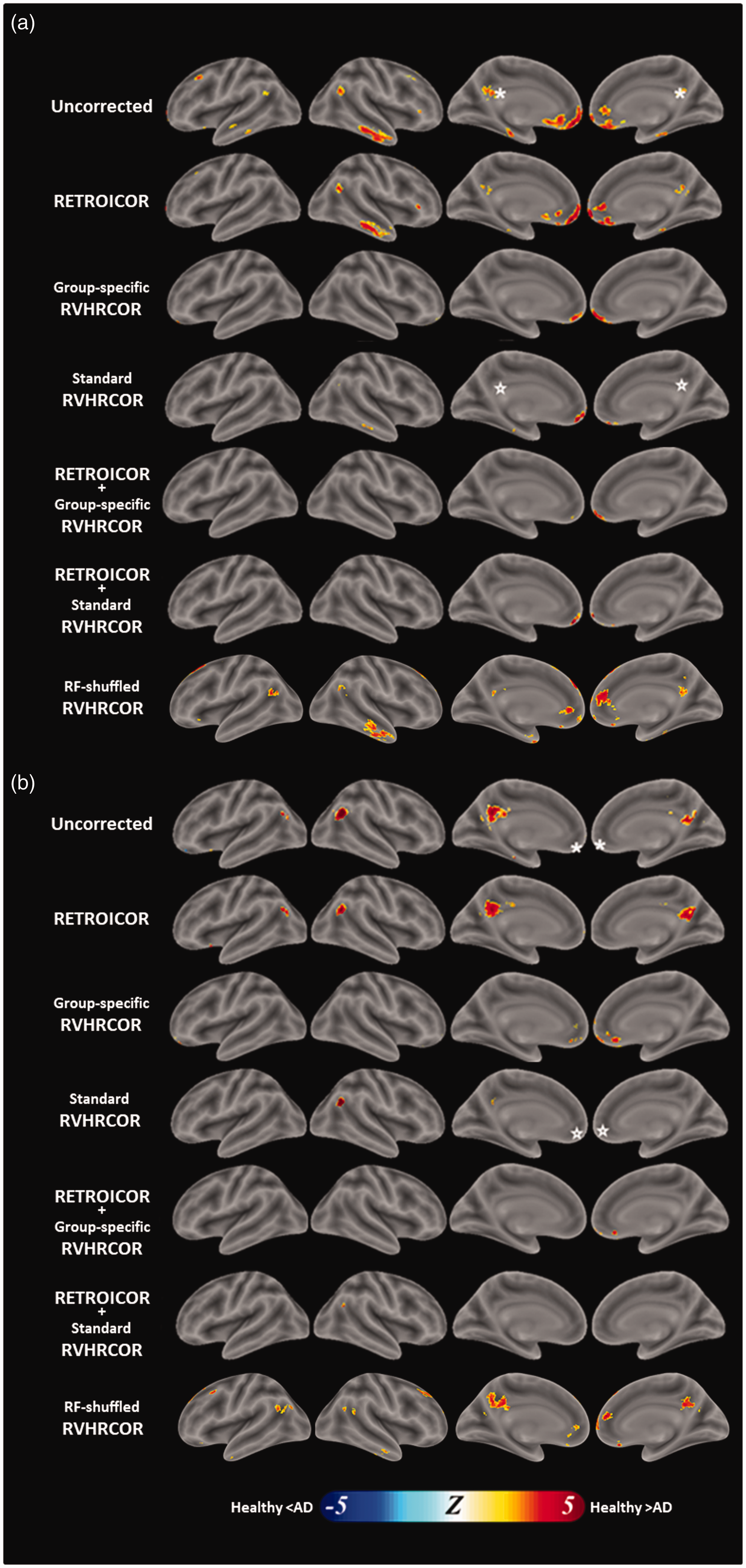
Statistical difference of physiological noise suppression on DMN identification between healthy participants and AD patients. This is the comparison between healthy (left) and AD cohorts (right) in Figure 5. The DMN was estimated by data without physiological noise suppression, with RETROICOR, with group-specific RVHRCOR, with both RETROICOR and group-specific RVHRCOR, and with both RETROICOR and standard RVHRCOR using PCC (a) and mPFC (b) as the seed region. The significance level was p < 0.05 after controlling the false discovery rate. White asterisks denote the location of the seed regions.

As to the comparison between standard RVHRCOR and group-specific RVHRCOR, we found that using group-specific response functions caused (1) reduced DMN difference between AD patients and healthy participants in the right temporal cortex when taking the PCC as the seed, (2) reduced DMN difference between AD patients and healthy participants at right LPL when taking the mPFC as the seed, and (3) increased DMN difference between AD patients and healthy participants at a few sporadic locations around the medial frontal lobe when taking the mPFC as the seed.

DMN’s difference before and after physiological noise suppression

The DMN differences between the estimate using data with and without physiological noise suppression are shown in Figure 7. It depicts how physiological noise suppression affects the functional connectivity within a group. Significant changes caused by suppressing physiological noise were found both inside and outside the DMN: physiological noise suppression (RETROICOR + group-specific RVHRCOR) significantly reduced the functional connectivity with PCC at the right frontal lobe, bilateral LPLs, bilateral temporal poles, mPFC, precuneus, and several other locations outside the DMN in healthy participants. Such a reduction in functional connectivity with PCC was also found in AD patients at bilateral mPFC, sensorimotor cortices, and the frontal poles.

Figure 7.

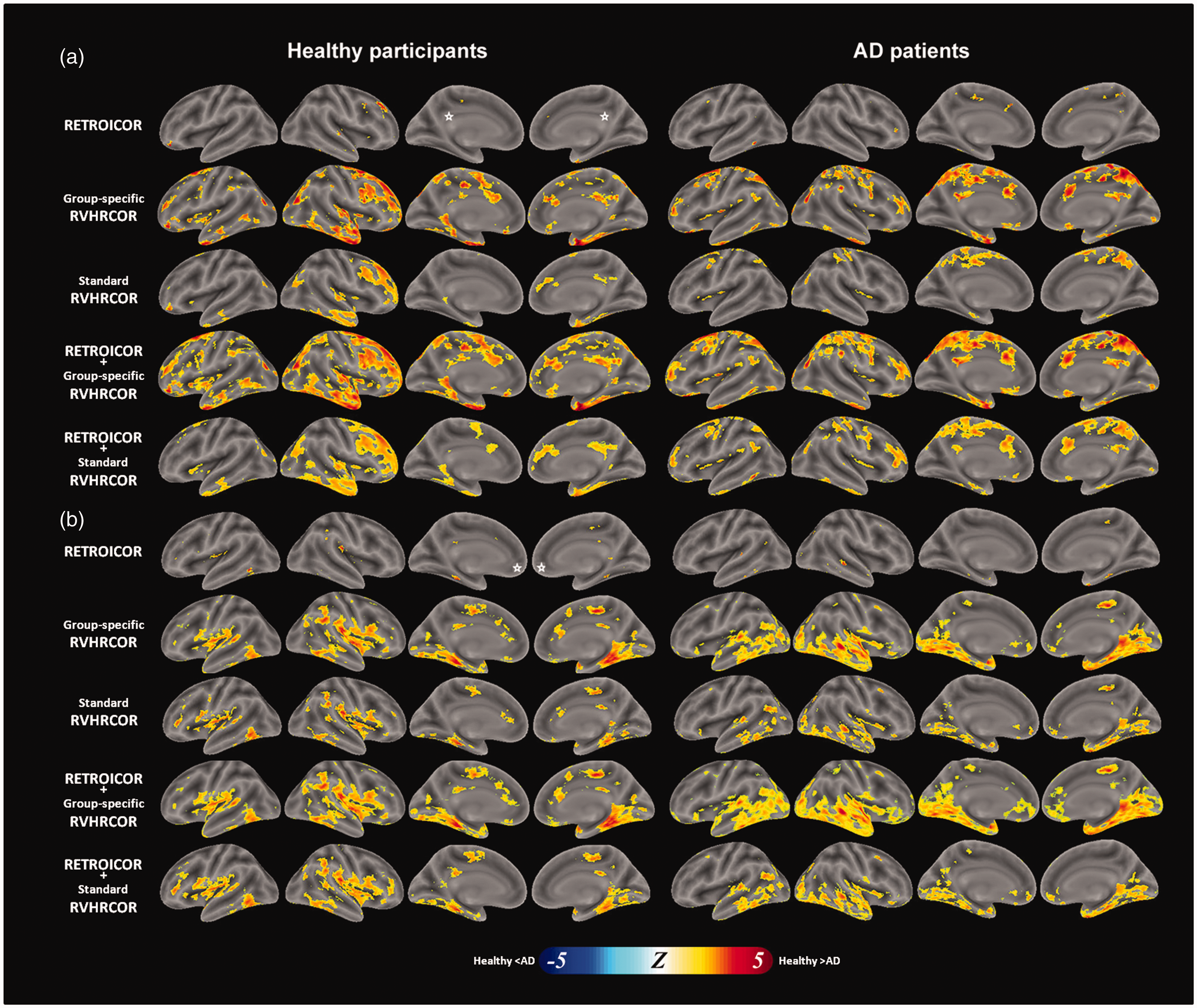
The DMN difference after methods of physiological noise suppression for healthy participants (left) and AD patients (right) using PCC (a) or mPFC (b) as the seed region. The comparison was made with respect to the DMN without physiological noise suppression. Methods of physiological noise suppression include RETROICOR (top row), group-specific RVHRCOR (the 2nd row), the combination of RETROICOR and group-specific RVHRCOR (the 3rd row), and the combination of RETROICOR and standard RVHRCOR (bottom row). The significance level was p < 0.05 after controlling the false discovery rate. White asterisks denote the location of the seed regions.

Taking mPFC as the seed region, physiological noise suppression (RETROICOR + group-specific RVHRCOR) reduced the functional connectivity near bilateral parahippocampal gyrus, PCC, supplementary motor area, bilateral insula, and right LPL in healthy participants. Physiological noise suppression (RETROICOR + group-specific RVHRCOR) reduced the DMN at bilateral LPL and ventral occipital lobes, superior temporal gyrus, medial temporal gyrus, insula, and parahippocampal gyrus in AD patients. Regardless of the seed region and the subject group, applying group-specific RVHRCOR caused more DMN changes than applying RETROICOR. A larger change was made by using both RETROICOR and group-specific RVHRCOR than using both RETROICOR and standard RVHRCOR.

Discussion

This study investigated how physiological noise affects the characterization of the resting-state DMN between AD patients and healthy participants. Compared to healthy participants, AD patients had significant delays in the hemodynamic responses to cardiac and respiratory cycles (Figure 1). These findings suggested the pathophysiological modulation on hemodynamic responses related to heart rhythms and breathing. Delayed RRF and CRF in AD patients may be attributed to the dysfunction of neurovascular coupling. Significant tSNR improvement in the fMRI data can be obtained after removing the hemodynamic changes caused by heart beating and breathing from the fMRI time series (Figures 2 to 4). The topology of the DMN was successfully identified (Figure 5). However, the difference in DMN between healthy participants and AD patients using data after physiological noise suppression became less significant (Figures 6). The DMN identification and the difference in the DMN between healthy participants and AD patients matched previous studies using fMRI data without physiological noise suppression.^10–13,35 No significant DMN’s difference between the RF-shuffled RVHRCOR and the uncorrected results (Figure 7). The result suggested that our functional connectivity estimates were minimally attributed to the degree of freedom. Collectively, our results demonstrated how controlling physiological noise affects DMN characterization, particularly when contrasting between disease states. Specifically, group-specific denoising reduced the DMN difference. Based on current findings, we suggest to properly denoise fMRI using group-specific response function in order to attribute the DMN more specifically to its neurophysiological origin. We want to emphasize that this study does not suggest the DMN is similar between AD patients and healthy participants. Instead, we would like to bring a cautious note that the difference in DMN between AD patients and healthy subjects can be erroneously inflated if physiological noise is not appropriately controlled. Caution should be taken when using fMRI DMN as an imaging marker to differentiate between two population groups if physiological noise is not properly suppressed.

RETROICOR was performed after spatial normalization and before slice timing correction. Such a procedure was recommended by a previous study.³² RETROICOR and RVHRCOR reduced different fluctuations in a BOLD waveform. Specifically, RETROICOR estimated phase-locked fluctuations in the BOLD waveform by fitting it to a low-order Fourier series. On the other hand, RVHRCOR modeled BOLD fluctuations related to breathing depth and heart rate variability. In our data processing, RVHRCOR was done after RETROICOR. This order was suggested by a previous study,²⁰ which also showed that reversing the order of RETROICOR and RVHRCOR made little difference in the effect of physiological noise suppression.

The regions showing significant improvement with RETROICOR were sparsely distributed over the brain (Figure 3). The sparse distribution of the RETROICOR improvement was consistent with a previous study.³⁶ The RETROICOR method accounts for physiological noise influences from distant pulsatile blood vessels (Circle of Willis), while the RVHRCOR method removes structured and temporally repeating physiological noise arising from the dense vasculature.³⁶ Compared to RVHRCOR, RETROICOR had relatively smaller effects, possibly because the cortical areas examined in this study were relatively distant from the source of pulsatile blood vessels.³⁶

In this study, we used both RETROICOR and the regression with WM and CSF time series to reduce the physiological noise. This combined approach may raise the concern about introducing noise back into the data, as they both dealt with some common noise effects. However, we would like to point out one important difference between RETROICOR and WM/CSF regression related to this concern: the removed signal in WM/CSF regression had an intact temporal structure as that in the acquired fMRI time series, while the removed signal in RETROICOR was temporally shuffled based on cardiac and respiratory phases. The difference in the temporal structure of the time series in WM/CSF regression and RETROICOR (intact vs. shuffled) made the concern of increasing the noise when performing both corrections less likely. Additionally, studies suggested that the RETROICOR accounts for the most variance in pulsatile blood vessels near the base of the brain and the circle of Willis³⁷ and the brainstem,^38,39 while the WM/CSF regression has relatively less spatial specificity. The spatiotemporal difference between WM/CSF regression and RETROICOR suggested that both methods can work together without artificially inflating the noise. To empirically test our argument, we performed only RETROICOR without WM/CSF regression. We found that the tSNR difference between RETROICOR without WM/CSF regression (Figure 3, the top row) and RETROICOR with WM/CSF regression (Figure 3, the 2nd row) was relatively minor, suggesting that WM/CSF regression and RETORICOR can be used together without inflating the noise. These results were consistent with previous studies^37,40 using both WM/CSF regression and RETROICOR to suppress the physiological noise.

In our study, we used RV²⁰ rather than respiratory volume per time (RVT)²⁸ to model the hemodynamic response related to breathing. RV was derived from the standard deviation of the respiratory waveform on a sliding window of 3 TRs (6 s) centered at each TR. The RV measure is easier to derive and more robust to noise than RVT, as it calculates the RMS average fluctuation over a window rather than taking a single peak-to-valley difference. Thus, RV does not depend on the accuracy of peak detection, which is required for breath-to-breath computations.²⁰ A previous study shows that RV measure was correlated with RVT, and the average RV transfer function agreed with the RVT transfer function.²⁰ The analysis using RV yielded similar results to those using RVT.²⁹

Three recent studies^41–43 explicitly considered the time lag of the cardiac/respiratory response functions. In this study, we also estimated the latency of the response function. Physiological response functions with different latencies were then used to remove physiological noise (Figure 6). While using a different approach, our results can be similar to what would be obtained by other approaches.

In addition to the respiration depth and heart rate variabilities, fluctuations in the end-tidal CO₂ (PETCO₂) can also cause noise in resting-state fMRI signal. This artifact has been characterized in healthy adults.^44,45 The spatial pattern of the PETCO₂ effect was found similar to that of RV.⁴⁴ Thus, we speculated that suppressing the physiological noise modeled by both RV and HR in this study may partially account for the effects related to PETCO₂. This speculation needs further experiments to verify.

While the phase-dependent physiological responses are likely to be related to pressure-changes and tissue motion caused by respiration and pulsation, the phase-independent effects related to the cardiac frequency or respiratory depth are of more uncertain origins. In this study, we speculated that the origin of these effects is vascular. However, there are also studies suggesting the potential neuronal mechanisms underpinning the fMRI timing difference between the healthy and AD cohorts. Specifically, RVT and HR have been found associated with vigilance and autonomic nervous control,^46,47 respectively. Attributing RVT and HR as vascular noise can be overly simplified. Clarifying the physiological origin of these effects is beyond the scope of this study. We plan to pursue this topic in the next study.

In addition to the seed-based correlation method, independent component analysis (ICA) can also analyze the resting-state fMRI data. Using fMRI data collected on a 1.5 T scanner, Starck et al.⁴⁸ have applied ICA to separate both DMN and low-frequency fluctuations. However, they found little difference between DMNs characterized by data before and after physiological noise suppression. This discrepancy from our results may be due to the fact that the physiological noise was smaller at 1.5 T than at 3 T.¹⁸ It may be argued that physiological noise suppression was not as important as what we found in the seed-based analysis because ICA automatically classifies the whole fMRI data into signal and noise components, including components associated with the physiological noise. However, such an argument was built upon the assumption that the DMN and the spatial patterns associated with physiological noise were spatially independent. Nevertheless, this assumption is directly challenged by a previous study showing the significant overlap between the DMN and areas showing a significant correlation between local hemodynamic responses and respiratory depth.²⁸ Taken together, we suggest that estimating DMN by ICA should consider using the data after physiological noise suppression in order to minimize the effects related to cardiac and respiratory cycles.

Physiological response functions

In RVHRCOR, the RV and the HR regressors were computed by convolving the RV or the HR waveforms with RRF and CRF, respectively. Note that the ages of participants in those two published studies^20,28 were much younger than ours (31.8 and 31.4 years old, respectively; our study: 77 years old). Participants at different ages may have different physiological response functions. Using the same physiological response functions for participants across different ages may confound the analyses.

Previously, it has been suggested that AD patients had abnormal neurovascular coupling²⁶ due to cerebral blood flow alteration possibly caused by the cerebrovascular disease and the amyloid-beta (Aβ) plaque deposition.^49,50 The change in neurovascular coupling can cause BOLD response delay.⁵¹ Our results directly support this hypothesis by showing (1) a more delayed physiological response functions in AD patients (Figure 1), and (2) significantly improved tSNR across the whole brain after removing hemodynamic responses to cardiac and respiratory response functions using RVHRCOR (Figure 3).

In this study, we obtained group-specific RRF and CRF for physiological noise suppression. While it is possible to estimate participant-specific RRF and CRF, such estimates can be less reliable, because the data size will be decreased dramatically (from n participants to 1). Even so, we still estimated the participant-specific RRF and CRF and then averaged across participants (Supplementary Figure 3). In fact, both methods showed delayed RRF and CRF in the AD patient group (group-specific RFs: Figure 1; participant-specific RFs: Supplementary Figure 3). However, the group-specific response functions showed a smaller variance, potentially due to the pooled data in RF estimation. Consequently, we took group-specific RRF and CRF in this study.

A previous study suggested that effective connectivity estimates can be biased by hemodynamic response function estimates.⁵² Here, we show that an inaccurate physiological response function can bias functional connectivity estimates. A more accurate estimate of the physiological response function should improve the sensitivity and specificity of using functional connectivity to characterize the difference between groups. We understand that the RRF and CRF can vary not only across participants but also across brain areas. However, in this study, we only estimated one set of RRF and CRF for a group of participants because of the trade-off between the stability of RRF/CRF estimates and their variabilities across participants and brain areas. We concatenated the time series from brain areas significantly affected by RRF and CRF during iterative RRF and CRF estimation. This data pooling increased the signal-to-noise ratio of the RRF and CRF estimates at the cost of ignoring region-specific CRF and RRF features.

Even the RRF and CRF latencies may vary spatially, how these latency differences affect the residual fMRI time series, and the subsequent functional connectivity estimates are yet to be studied systematically. Our results show that functional connectivity was weaker after physiological noise suppression (Figure 5). If considering the true functional connectivity due to neuronal activity is confounded by hemodynamic fluctuations, our results can be explained by the fact that we used the same, but sub-optimal estimated CRF and RRF waveforms to suppress noise across the whole brain inefficiently. With CRF and RRF estimates varying between locations, we may better suppress these hemodynamic fluctuations more efficiently and consequently have higher functional connectivity between target and seed regions. In other words, the reduced functional connectivity found in our study can be attributed to the sub-optimal and spatially invariant physiological response function estimates, which were, nevertheless, taken in this study because of the signal-to-noise ratio concerns.

tSNR improvement and DMN characterization

Using group-specific RVHRCOR caused more tSNR improvement in both healthy participants and AD patients than using standard RVHRCOR (Figure 3). Such a tSNR improvement caused more specific DMN characterization (Figure 5). As DMN estimates were more specific after removing contributions from RV and HR variability, the difference in DMN between healthy participants and AD patients is reduced (Figures 6). Overall, we found that the tSNR improvement in the resting-state fMRI data by suppressing the physiological noise significantly affects DMN characterization. However, the tSNR measure should be taken cautiously, because it can be improved by over suppression of the fMRI signal fluctuation at the cost of reduced detection of functionally connected networks.⁵³ The denoising processes can accidentally suppress both noise and signal. However, we attempted to avoid such over-fitting (to noise) by using the same physiological response functions (CRF and RRF) across participants in the same population group. We acknowledged that tSNR is neither the only nor the best means for assessing the quality of resting-state fMRI data. Caution must be taken in interpreting tSNR after different processing.

In conclusion, our study exemplifies the need to suppress the physiological noise in the fMRI data. This is particularly important in studying fMRI data collected from neurological/psychiatric diseases patients, such as hypertension, stroke, AD, and other cerebral vascular diseases,^26,49 where there exist pathophysiological changes in the vasculature, vascular reactivity, or neurovascular coupling.

Supplemental Material

JCB897442 Supplemental material - Supplemental material for Impact of physiological noise in characterizing the functional MRI default-mode network in Alzheimer’s disease

Supplemental material, JCB897442 Supplemental material for Impact of physiological noise in characterizing the functional MRI default-mode network in Alzheimer’s disease by Yi-Tien Li, Chun-Yuan Chang, Yi-Cheng Hsu, Jong-Ling Fuh, Wen-Jui Kuo, Jhy-Neng Tasso Yeh and Fa-Hsuan Lin in Journal of Cerebral Blood Flow & Metabolism

Footnotes

Funding

The author(s) disclosed receipt of the following financial support for the research, authorship, and/or publication of this article: This work was partially supported by Ministry of Science and Technology, Taiwan (103-2628-B-002-002-MY3, 105-2221-E-002-104), National Health Research Institute (NHRI-EX107-10727EI), and the Academy of Finland (No. 298131).

Acknowledgment

We thank Dr. Shih-Wei Wu’s comments on the manuscript.

Declaration of conflicting interests

The author(s) declared no potential conflicts of interest with respect to the research, authorship, and/or publication of this article.

Authors’ contributions

Lin F-H and Kuo W-J designed the experiment. Li Y-T, Hsu Y-C, and Yeh J-N analyzed data. Chang C-Y, Fuh J-L, and Li Y-T interpreted the patient data. Li Y-T and Lin F-H were major contributors in writing the manuscript. All authors read and approved the final manuscript.

Supplemental material

Supplemental material for this article is available online.

ORCID iD

Yi-Tien Li

References

Yee

S-H

Liu

H-L

Hou

, et al. Detection of the brain response during a cognitive task using perfusion‐based event‐related functional MRI. Neuroreport 2000; 11: 2533–2536.

Biswal

Yetkin

Haughton

, et al. Functional connectivity in the motor cortex of resting human brain using echo-planar MRI. Magn Reson Med 1995; 34: 537–541.

Cole

Smith

Beckmann

CF.

Advances and pitfalls in the analysis and interpretation of resting-state FMRI data.

Front Syst Neurosci 2010; 4: 8.

Rosazza

Minati

Resting-state brain networks: literature review and clinical applications.

Neurol Sci 2011; 32: 773–785.

Buckner

Andrews‐Hanna

Schacter

DL.

The brain's default network: anatomy, function, and relevance to disease. Ann N Y Acad Sci 2008; 1124: 1–38.

Fox

Snyder

Vincent

, et al. The human brain is intrinsically organized into dynamic, anticorrelated functional networks. Proc Natl Acad Sci U S A 2005; 102: 9673–9678.

Ghatan

Hsieh

Wirsén-Meurling

, et al. Brain activation induced by the perceptual maze test: a PET study of cognitive performance. Neuroimage 1995; 2: 112–124.

Hutchinson

Schiffer

Joseffer

, et al. Task-specific deactivation patterns in functional magnetic resonance imaging. Magn Reson Imag 1999; 17: 1427–1436.

Gusnard

Raichle

ME.

Searching for a baseline: functional imaging and the resting human brain.

Nat Rev Neurosci 2001; 2: 685–694.

10.

Allen

Bernard

McColl

, et al. Reduced hippocampal functional connectivity in Alzheimer disease. Arch Neurol 2007; 64: 1482–1487.

11.

Rombouts

Barkhof

Goekoop

, et al. Altered resting state networks in mild cognitive impairment and mild Alzheimer's disease: an fMRI study. Hum Brain Mapp 2005; 26: 231–239.

12.

Wang

Zang

, et al. Changes in hippocampal connectivity in the early stages of Alzheimer's disease: evidence from resting state fMRI. Neuroimage 2006; 31: 496–504.

13.

Wang

Liang

Wang

, et al. Altered functional connectivity in early Alzheimer's disease: a resting-state fMRI study. Hum Brain Mapp 2007; 28: 967–978.

14.

Zhang

Rane

Huang

, et al. Mapping resting-state brain networks in conscious animals. J Neurosci Meth 2010; 189: 186–196.

15.

Greicius

Srivastava

Reiss

, et al. Default-mode network activity distinguishes Alzheimer's disease from healthy aging: evidence from functional MRI. Proc Nat Acad Sci U S A 2004; 101: 4637–4642.

16.

Sheline

Raichle

Snyder

, et al. Amyloid plaques disrupt resting state default mode network connectivity in cognitively normal elderly. Biol Psychiatry 2010; 67: 584–587.

17.

Krüger

Glover

GH.

Physiological noise in oxygenation‐sensitive magnetic resonance imaging.

Magn Reson Med 2001; 46: 631–637.

18.

Triantafyllou

Hoge

Krueger

, et al. Comparison of physiological noise at 1.5 T, 3 T and 7 T and optimization of fMRI acquisition parameters. Neuroimage 2005; 26: 243–250.

19.

Hutton

Josephs

Stadler

, et al. The impact of physiological noise correction on fMRI at 7 T. Neuroimage 2011; 57: 101–112.

20.

Chang

Glover

GH.

Effects of model-based physiological noise correction on default mode network anti-correlations and correlations.

Neuroimage 2009; 47: 1448–1459.

21.

Fischer

Siddiqi

Yusufaly

Altered angioarchitecture in selected areas of brains with Alzheimer's disease.

Acta Neuropathol 1990; 79: 672–679.

22.

Kalaria

Hedera

Differential degeneration of the cerebral microvasculature in Alzheimer's disease.

Neuroreport 1995; 6: 477–480.

23.

Mazza

Marano

Traversi

, et al. Primary cerebral blood flow deficiency and Alzheimer's disease: shadows and lights. J Alzheimers Dis 2011; 23: 375–389.

24.

Asemani

Morsheddost

Shalchy

MA.

Effects of ageing and Alzheimer disease on haemodynamic response function: a challenge for event-related fMRI.

Healthcare Technol Lett 2017; 4: 109–114.

25.

Winter

Bludszuweit-Philipp

Wolkenhauer

Mathematical analysis of the influence of brain metabolism on the BOLD signal in Alzheimer’s disease.

J Cereb Blood Flow Metab 2018; 38: 304–316.

26.

Girouard

Iadecola

Neurovascular coupling in the normal brain and in hypertension, stroke, and Alzheimer disease.

J Appl Physiol 2006; 100: 328–335.

27.

Satterthwaite

Elliott

Gerraty

, et al. An improved framework for confound regression and filtering for control of motion artifact in the preprocessing of resting-state functional connectivity data. Neuroimage 2013; 64: 240–256.

28.

Birn

Smith

Jones

, et al. The respiration response function: the temporal dynamics of fMRI signal fluctuations related to changes in respiration. Neuroimage 2008; 40: 644–654.

29.

Chang

Cunningham

Glover

GH.

Influence of heart rate on the BOLD signal: the cardiac response function.

Neuroimage 2009; 44: 857–869.

30.

Friston

Fletcher

Josephs

, et al. Event-related fMRI: characterizing differential responses. Neuroimage 1998; 7: 30–40.

31.

Gary

H and

Glover

T-QLaR.

Image-based method for retrospective correction of physiological motion effects in fMRI: RETROICOR.

Magn Reson Med 2000; 44: 162–167.

32.

Jones

Bandettini

Birn

RM.

Integration of motion correction and physiological noise regression in fMRI.

Neuroimage 2008; 42: 582–590.

33.

Margulies

Kelly

Uddin

, et al. Mapping the functional connectivity of anterior cingulate cortex. Neuroimage 2007; 37: 579–588.

34.

Gorges

Müller

H-P

Lulé

, et al. Functional connectivity within the default mode network is associated with saccadic accuracy in Parkinson's disease: a resting-state fMRI and videooculographic study. Brain Connect 2013; 3: 265–272.

35.

Zhang

Raichle

ME.

Disease and the brain's dark energy.

Nat Rev Neurol 2010; 6: 15–28.

36.

Krishnamurthy

Schwam

, et al. Retrospective correction of physiological noise: impact on sensitivity, specificity, and reproducibility of resting-state functional connectivity in a reading network model. Brain Connect 2018; 8: 94–105.

37.

Birn

Cornejo

Molloy

, et al. The influence of physiological noise correction on test–retest reliability of resting-state functional connectivity. Brain Connect 2014; 4: 511–522.

38.

Brooks

JCW

Faull

Pattinson

, et al. Physiological noise in brainstem FMRI. Front Hum Neurosci 2013; 7: 623.

39.

Harvey

Pattinson

Brooks

, et al. Brainstem functional magnetic resonance imaging: disentangling signal from physiological noise. J Magn Reson Imaging 2008; 28: 1337–1344.

40.

Bartoň

Mareček

Krajčovičová

, et al. Evaluation of different cerebrospinal fluid and white matter fMRI filtering strategies – quantifying noise removal and neural signal preservation. Hum Brain Mapp 2019; 40: 1114–1138.

41.

Pinto

Nunes

Bianciardi

, et al. Improved 7 Tesla resting-state fMRI connectivity measurements by cluster-based modeling of respiratory volume and heart rate effects. Neuroimage 2017; 153: 262–272.

42.

Birn

Cornejo

Molloy

, et al. The influence of physiological noise correction on test–retest reliability of resting-state functional connectivity. Brain Connect 2014; 4: 511–522.

43.

Bianciardi

Fukunaga

van Gelderen

, et al. Sources of functional magnetic resonance imaging signal fluctuations in the human brain at rest: a 7 T study. Magn Reson Imaging 2009; 27: 1019–1029.

44.

Golestani

Chang

Kwinta

, et al. Mapping the end-tidal CO2 response function in the resting-state BOLD fMRI signal: spatial specificity, test–retest reliability and effect of fMRI sampling rate. Neuroimage 2015; 104: 266–277.

45.

Golestani

Kwinta

Strother

, et al. The association between cerebrovascular reactivity and resting-state fMRI functional connectivity in healthy adults: the influence of basal carbon dioxide. Neuroimage 2016; 132: 301–313.

46.

Engelhardt

Laks

Alzheimer disease neuropathology: understanding autonomic dysfunction.

Dement Neuropsychol 2008; 2: 183–191.

47.

Ozbay

Chang

Picchioni

, et al.

Contribution of sympathetic vasoconstriction to the fMRI global signal during autonomic arousals.

Proc Intl Soc Mag Reson Med 2019; 27: 512.

48.

Starck

Remes

Nikkinen

, et al. Correction of low-frequency physiological noise from the resting state BOLD fMRI – effect on ICA default mode analysis at 1.5 T. J Neurosci Meth 2010; 186: 179–185.

49.

Carusone

Srinivasan

Gitelman

, et al. Hemodynamic response changes in cerebrovascular disease: implications for functional MR imaging. Am J Neuroradiol 2002; 23: 1222–1228.

50.

Zlokovic

BV.

Neurovascular pathways to neurodegeneration in Alzheimer's disease and other disorders.

Nat Rev Neurosci 2011; 12: 723–738.

51.

Rombouts

SARB

Goekoop

Stam

, et al. Delayed rather than decreased BOLD response as a marker for early Alzheimer's disease. Neuroimage 2005; 26: 1078–1085.

52.

G-R

Liao

Stramaglia

, et al. A blind deconvolution approach to recover effective connectivity brain networks from resting state fMRI data. Med Image Anal 2013; 17: 365–374.

53.

Bright

Murphy

Is fMRI “noise” really noise? Resting state nuisance regressors remove variance with network structure.

Neuroimage 2015; 114: 158–169.

Supplementary Material

Please find the following supplemental material available below.

For Open Access articles published under a Creative Commons License, all supplemental material carries the same license as the article it is associated with.

For non-Open Access articles published, all supplemental material carries a non-exclusive license, and permission requests for re-use of supplemental material or any part of supplemental material shall be sent directly to the copyright owner as specified in the copyright notice associated with the article.

0.00 MB

0.51 MB