Predicting 15 O-Water PET cerebral blood flow maps from multi-contrast MRI using a deep convolutional neural network with evaluation of training cohort bias

Abstract

To improve the quality of MRI-based cerebral blood flow (CBF) measurements, a deep convolutional neural network (dCNN) was trained to combine single- and multi-delay arterial spin labeling (ASL) and structural images to predict gold-standard ¹⁵O-water PET CBF images obtained on a simultaneous PET/MRI scanner. The dCNN was trained and tested on 64 scans in 16 healthy controls (HC) and 16 cerebrovascular disease patients (PT) with 4-fold cross-validation. Fidelity to the PET CBF images and the effects of bias due to training on different cohorts were examined. The dCNN significantly improved CBF image quality compared with ASL alone (mean ± standard deviation): structural similarity index (0.854 ± 0.036 vs. 0.743 ± 0.045 [single-delay] and 0.732 ± 0.041 [multi-delay], P < 0.0001); normalized root mean squared error (0.209 ± 0.039 vs. 0.326 ± 0.050 [single-delay] and 0.344 ± 0.055 [multi-delay], P < 0.0001). The dCNN also yielded mean CBF with reduced estimation error in both HC and PT (P < 0.001), and demonstrated better correlation with PET. The dCNN trained with the mixed HC and PT cohort performed the best. The results also suggested that models should be trained on cases representative of the target population.

Introduction

Cerebral blood flow (CBF) is the fundamental rate constant of the brain, determining the delivery of oxygen and other nutrients, the lysis of microclots, and the removal of waste products. Adequate CBF is essential for neurological health and is altered in many diseases, including cerebrovascular diseases. In addition, evidence suggests that CBF changes are important in other disorders, such as neurodegenerative disease and multiple sclerosis.^1,2 Even though it is crucial to monitor CBF changes, imaging methods to assess perfusion remain underdeveloped. ³ Reference standard methods such as ¹⁵O-water positron emission tomography (¹⁵O-water PET) and Xenon-enhanced CT (XeCT) are laborious to implement and are not FDA-approved. Furthermore, they require radiation and thus cannot be obtained in large cohorts. As such, establishing a radiation- and contrast-free quantitative CBF method that is robust and accurate even in severe, large vessel arterial disease is a high priority.

Arterial spin labeling (ASL) is an MRI method that enables CBF measurement without contrast.^4,5 Much progress has been made over the past decade, culminating in consensus guidelines for clinical application of ASL. ⁶ However, the risk of underestimating local CBF in cerebrovascular disease patients as well as the underlying low signal-to-noise ratio (SNR) of the technique call for new approaches. ⁷ These include new pulse sequences such as extremely long-label long-delay, ⁸ multi-delay,^9–11 and velocity-selective labeling,^12–14 which address the problem of imaging slow flow. However, all of these methods still have limited accuracy to measure CBF in cerebrovascular disease patients with long transit delays. ¹⁵O-water PET is considered the “gold standard” for CBF quantification, has high SNR, and is less sensitive to arrival times. However, due to the requirements mentioned above, PET is not feasible in most clinical settings.

Recently, deep convolutional neural networks (dCNN) have shown superior performance to other machine learning techniques on image recognition tasks ¹⁵ and more recently have been applied in medical imaging,^16–20 including image reconstruction, improving the quality of medical images, and synthesizing image contrasts from a different imaging modality. Although dCNNs have shown utility in ASL de-noising,^21,22 the current methods have yet to address the issue of regional CBF estimation bias and error due to slow flow and/or pathology. In improving medical image quality, a critical question is whether a dCNN needs to train on examples of pathology to successfully predict pathology when it is deployed on a separate group of patients. In our task to predict CBF, it is important to know whether a dCNN trained only on healthy controls would generalize to a patient cohort comprised of patients with cerebrovascular disease. Any potential prediction bias when the training and prediction were performed on cohorts with different distribution characteristics should be carefully evaluated and has implications well beyond CBF prediction for medical imaging. ²³

In this study, we propose a deep learning-based method that takes multiple MRI scans, including ASL, as inputs to predict a simultaneously obtained ¹⁵O-water PET CBF map. If such a method can be validated, the parameters of the model can be used in patients who receive only MRI to produce more accurate CBF maps, allowing higher quality CBF imaging in settings without the capability to perform ¹⁵O-water PET scans.

Materials and methods

Image acquisition and data preprocessing

This is a retrospective study, approved by the Institutional Review Board of the Stanford University in accordance with the ethical standards of the Helsinki declaration of 1975/1983, and HIPAA compliant. All patients provided written consent prior to the study. Some of the patients participated in a previous study described in Fan et al. ⁸ Thirty-two subjects underwent simultaneous time-of-flight enabled 3.0 T PET/MRI (SIGNA, GE Healthcare, Milwaukee, WI, USA) with injection of 490–960 MBq ¹⁵O-water for the purposes of CBF imaging. The group included 16 healthy controls (HC) and 16 cerebrovascular disease patients (PT, 13 with Moyamoya disease and 3 with atherosclerotic steno-occlusive disease of the carotid arteries). The demographics of the subjects are summarized in Table 1. Each scan included one CBF measurement at baseline, and one 20 min after injection of a vasodilator (acetazolamide, 15 mg/kg IV).

Table 1.

Demographics of the subjects included in this study.

Healthy controls
Number	Sex	Age
16	9 F/7 M	41.4 ± 12.0 (22–62)
Patients
PT #	Sex	Age	Disease
1	M	74	ASD; right CCA stenosis, right VA occlusion.
2	F	25	MMD; bilateral MCA occlusion.
3	F	49	MMD; right M1 occlusion, left ICA stenosis.
4	F	38	MMD; left ICA stenosis, left A1 stenosis.
5	M	33	MMD; bilateral occlusion of supraclinoid ICA.
6	M	46	MMD; right ICA stenosis, right MCA occlusion.
7	F	46	MMD; stenosis of supraclinoid ICA, right M1, and right A1.
8	F	66	ASD; left ICA occlusion.
9	M	34	MMD; bilateral supraclinoid ICA occlusion.
10	M	34	MMD; bilateral occlusion of ICA, early termination of posterior artery.
11	F	35	MMD; bilateral ICA occlusion.
12	M	52	MMD; right ICA stenosis, occlusion of right M1 MCA.
13	F	34	MMD; right M1 occlusion, left M1 stenosis.
14	F	16	MMD; bilateral ICA stenosis, M1 occlusion.
15	F	26	MMD; bilateral stenosis of supraclinoid ICA.
16	M	73	ASD; proximal right ICA stenosis.
Summary	9 F/7 M	42.6 ± 16.9 (16–74)

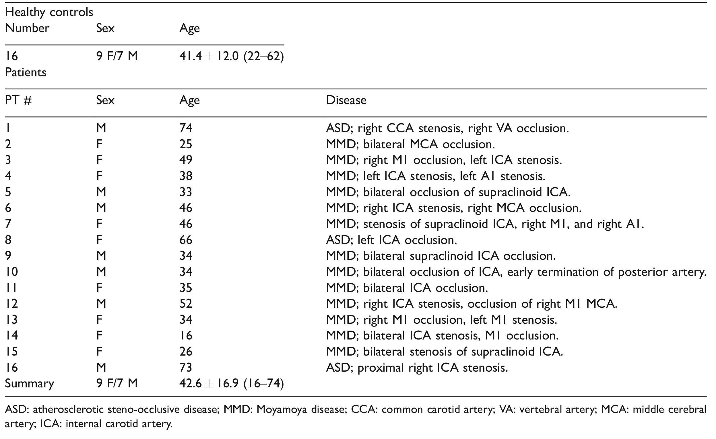
ASD: atherosclerotic steno-occlusive disease; MMD: Moyamoya disease; CCA: common carotid artery; VA: vertebral artery; MCA: middle cerebral artery; ICA: internal carotid artery.

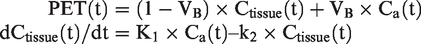
The PET images were reconstructed with a resolution of 1.56 × 1.56 × 2.78 mm³ and were corrected for ¹⁵O-water tracer signal decay, attenuation, scatter, random counts, and dead time. The quantitative PET CBF maps were generated using an image-derived input function (IDIF) method ²⁴ and Zhou’s one-tissue compartment model ²⁵ using PMOD software:

$$\begin{array}{l}\text{PET}\left(\text{t}\right)=\left(\text{1}-{\text{V}}_{\text{B}}\right)\times {\text{C}}_{\text{tissue}}\left(\text{t}\right)+{\text{V}}_{\text{B}}\times {\text{C}}_{\text{a}}\left(\text{t}\right)\\ {\text{dC}}_{\text{tissue}}\left(\text{t}\right)/\text{dt}={\text{K}}_{\text{1}}\times {\text{C}}_{\text{a}}\left(\text{t}\right)–{\text{k}}_{\text{2}}\times {\text{C}}_{\text{tissue}}\left(\text{t}\right)\end{array}$$

where K₁ is the perfusion rate constant, k₂ is the clearance rate constant, V_B is the blood volume, C_tissue(t) is the tissue time activity curve for each pixel and C_a(t) is the arterial blood concentration over time estimated by the IDIF method. For attenuation correction, we used the manufacturer’s single-atlas-based method based on 2-point Dixon images. The PET CBF measurement in this study was not used in clinical reading.

The MRI scans included both ASL scans and structural imaging. ASL scans included single-delay pseudocontinuous ASL ²⁶ with labeling duration (LD) = 1.45 s, post-labeling delay (PLD) = 2.025 s, and acquisition resolution = 3.64 × 3.64 × 4 mm³; and a multi-delay (5-delay) ASL with LD = 2 s, PLD = 0.7, 1.275, 1.85, 2.425 and 3 s, and acquisition resolution = 5.52 × 5.52 × 4 mm³. Proton density (PD)-weighted reference images were collected for CBF quantification. Background suppression (BGS) was used in both ASL sequences and the labeling efficiency loss due to BGS (∼25%) was corrected in the quantification of CBF. ²⁷ The ASL images were reconstructed with an interpolated resolution of 1.88 × 1.88 × 4 mm³. For single-delay ASL, the CBF maps were quantified using the simplified equation from Alsop et al. ⁶ with T₁ decay correction performed with assumed arterial T₁ of 1.65 s. ⁶ For multi-delay ASL, arterial transit time (ATT) maps and ATT-corrected CBF maps were generated from a kinetic ASL signal model^9,28,29 with T₁ decay correction performed with assumed arterial and tissue T₁ of 1.65 s and 1.5 s, ³⁰ respectively

$$\begin{array}{l}{\text{S}}_{\text{ASL},\text{i}}=2\cdot {\text{M}}_{\text{t},0}\cdot \text{CBF}\cdot \alpha \cdot {\text{T}}_{1\text{t}}\cdot {\text{e}}^{-\frac{\text{ATT}}{{\text{T}}_{1\text{a}}}}\\ \cdot \left({\text{e}}^{\frac{-\max \left({\text{PLD}}_{\text{i}}-\text{ATT},0\right)}{{\text{T}}_{1\text{t}}}}–{\text{ e}}^{\frac{-\max \left({\text{PLD}}_{\text{i}}+{\text{LD}}_{\text{i}}-\text{ATT},0\right)}{{\text{T}}_{1\text{t}}}}\right)/\lambda \end{array}$$

where M_t,0 is fully relaxed brain tissue magnetization in equilibrium, $\alpha$ is the labeling efficiency (0.85), ²⁶ T_1t and T_1a are the T₁ of tissue and arterial blood, respectively, LD_i is the i-th LD, and $\lambda$ is the tissue-to-blood partition coefficient of water (0.9 ml/g). ³¹

T₁-weighted (T_1w) 3D structural and T₂-weighted (T_2w) FLAIR images were acquired with a resolution of 0.94 × 0.94 × 1 mm³ (repetition time (TR)/echo time (TE)/inversion time (TI) = 9.5/3.8/400 ms) and 0.47 × 0.47 × 5 mm³ (TR/TE/TI = 9500/141/2300 ms).

All images were co-registered to the T_1w structural images using Statistical Parametric Mapping software (SPM12), and then normalized to the Montreal Neurological Institute (MNI) brain template ³² with 2 mm isotropic resolution using Advanced Normalization Tools (ANTs) software. ³³ The brain was extracted using FSL software. ³⁴ To reduce computation requirements, all images were resized to 96 × 96.

Deep convolutional neural network

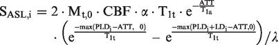
We developed a dCNN to synthesize high-quality, PET-like CBF maps from only MRI inputs including ASL. dCNN was chosen in this task because it is a powerful tool to efficiently extract and integrate intrinsic features in the input contrasts. The overall layout of the processing pipeline is shown in Figure 1(a). The detailed architecture of the dCNN is shown in Figure 1(b). We created a U-Net dCNN ³⁵ which includes three encoder layers and three decoder layers. Each encoder layer consists of three 2 D convolutional layers with a 3 × 3 kernel, a batch normalization layer, ³⁶ a rectifier linear unit (ReLU) activation layer, ³⁷ and a 2 × 2 maximum pooling (down-sampling) layer. A residual connection ¹⁹ is placed at the central layer. Each decoder layer consists a 2 × 2 up-sampling layer followed by three 2 D convolutional layers and ReLU activation layers. Bypassing shortcuts connect corresponding encoder-decoder layers to retain high-resolution information in the images. ³⁸

Figure 1.

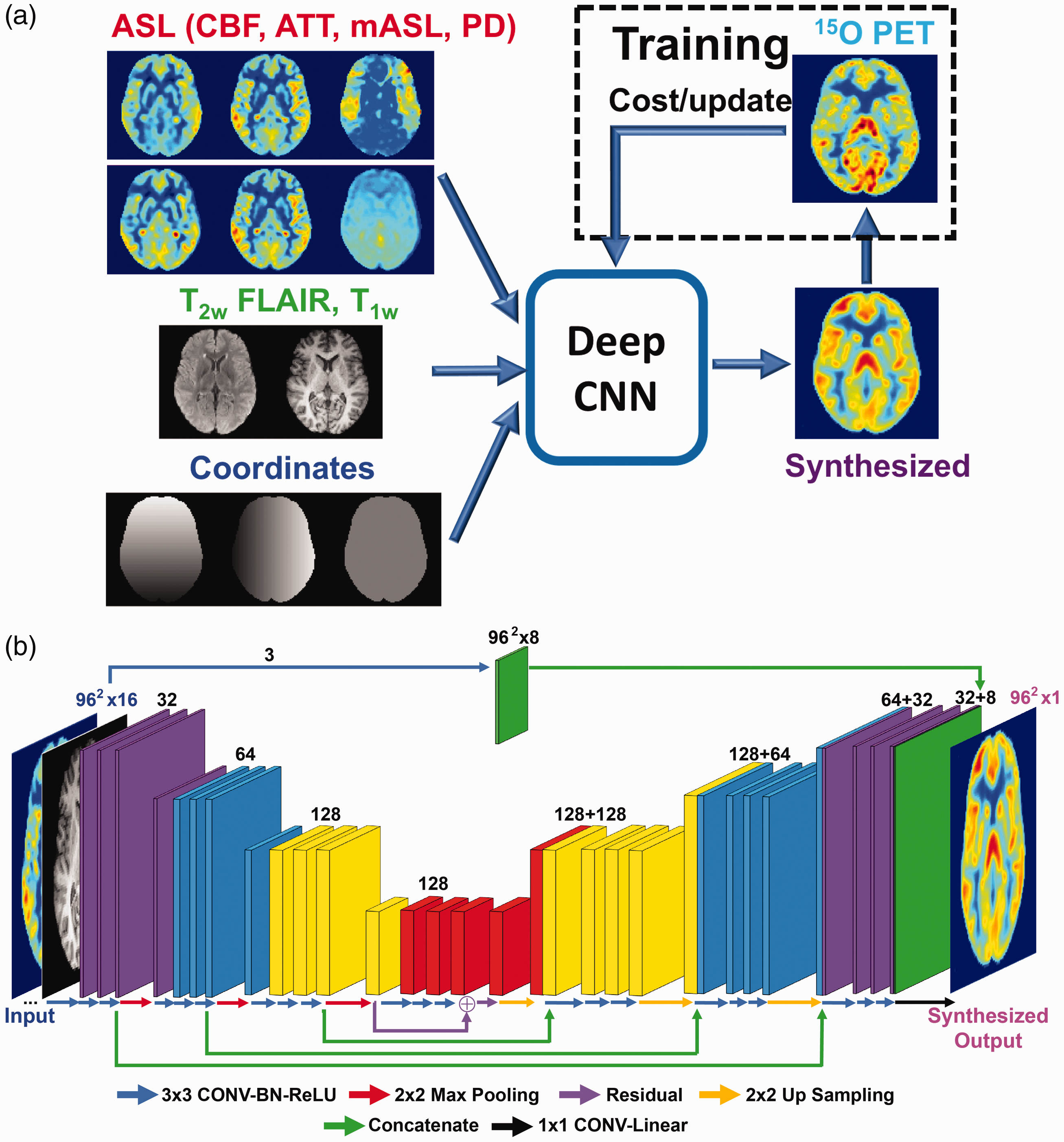
(a) Conceptual framework of the deep convolutional neural network (dCNN) methodology that combines multi-contrast MRI to improve cerebral blood flow (CBF) quantification; (b) the detailed network architecture of the dCNN, where the network components are color-coded and labeled at the bottom, and the input and output image dimensions are labeled. The channel numbers in each step are shown above the blocks. A detailed description of the network can be found in the text. CONV: convolutional layer; BN: batch normalization layer; ReLU: rectifier linear unit.

The input to the dCNN included 16 individual images: (1) ASL scans: quantitative CBF maps, mean ASL difference signal, PD_w reference images from both single-delay and multi-delay ASL scans, ATT maps and the raw ASL difference signal at each delay from multi-delay ASL; (2) structural scans: T_1w and T_2w FLAIR images; and (3) the pixel coordinate information in template space. To emphasize the perfusion information, the first three quantitative maps (CBF and ATT maps) were filtered by an additional convolution path (the path at the top in Figure 1(b)), and then appended to the last up-sampling layer of the U-Net before the final output. To improve convergence, all input images were normalized so that they had a mean intensity of 1 in the whole brain. The output of the dCNN was synthesized CBF maps that were normalized. During training, the synthesized CBF maps were compared with the reference ¹⁵O-water CBF images, using a cost function to minimize the mean absolute error, i.e. L1-norm, and update the parameters of the network. During testing, the input images directly passed through the fixed dCNN model to generate synthesized CBF maps. The synthesized normalized CBF maps were then scaled by the mean CBF values from the multi-delay ASL scans, which are more robust to transit delays than single-delay ASL, to yield the final quantitative CBF maps.

Model training and testing

A total of 64 PET/MRI datasets were included in this study, consisting of 62,720 images (excluding pixel coordinate information) before data augmentation, which was used to introduce controllable variations into and enlarge the size of the dataset. The augmentation included flipping along x and y directions, and a transpose within each slice of the input channels, resulting in a three-fold increase of the dataset size. Four-fold cross-validation was used in training and testing: the datasets were randomly divided into 4 sub-groups, each with 16 datasets from 4 HC and 4 PT. For each of the four trained dCNN models, the datasets from three sub-groups (48 datasets total) were used in training with 10% of the images randomly selected from shuffling for validation, and then the corresponding model was tested on the unused sub-group for performance evaluation. In addition, another set of training with the same cross-validation split was performed without the structural inputs to examine the effects of the structural input channels on the performance of the dCNN.

To examine the effect of potential training bias using different cohorts on the dCNN’s performance, the network was also trained on: (1) HC only, (2) PT only and (3) a mix of HC and PT with matched dataset size. Similar four-fold cross-validation aforementioned was used. For each HC-only (or PT-only) model, 24 HC (or PT) datasets in three sub-groups were used in training and tested on the unused sub-group, which contained both HC and PT datasets. For the mixed training dataset models, 12 HC and 12 PT datasets were randomly selected from three sub-groups, so a matched dataset size was achieved, which was half of that in the original mixed training. All training and testing were performed on a Linux system with a GTX 1080 Ti GPU (Nvidia, Santa Clara, CA). The training and validation losses were monitored to confirm that overfitting did not occur during training.

Image quality metrics, including structural similarity index (SSIM) ³⁹ and normalized root mean square error (NRMSE), were calculated by comparing the normalized ASL CBF and the PET reference maps, i.e. the CBF maps that have a mean intensity of 1 in the whole brain as described in the previous section. For accurate image quality assessment, five slices at the top and the bottom of the brain were excluded due to small numbers of brain voxels in these slices, leaving a total of 60 slices in each dataset. The SSIM and NRMSE were calculated in each slice, averaged across the whole brain and then compared in all subjects.

For quantification accuracy evaluation, mean regional cortical gray matter CBF values were calculated in 20 regions of interest (ROIs) derived from the Alberta Stroke Programme Early Computed Tomography Score (ASPECTS), ⁴⁰ corresponding to one anterior, three middle, and one posterior vascular territories per hemisphere, at each of the two slice locations, ⁴¹ within gray matter masks generated with the gray matter probability >0.8 in each voxel, and then compared with the corresponding PET reference values. The gray matter masks were applied on both ASL and PET CBF maps. The analysis was performed on both normalized (all subjects, normalization as defined above) and quantitative (some subjects excluded, see below) CBF maps.

As the IDIF method for PET quantification has not yet been extensively validated, to ensure a fair and informative comparison, the datasets suspected with PET quantification errors were identified and excluded from the analysis on quantification accuracy. The exclusion criteria included: (1) the datasets with error scores more than 1.5 × interquartile range above the third quartile or below the first quartile (six subjects excluded); to avoid bias for or against the dCNN method, the error scores were an average of NRMSE for single-delay ASL, multi-delay ASL and dCNN; and (2) failure of PET to detect CBF augmentation between pre- and post-acetazolamide injection in the cerebellum, which should be present in both HC and PT populations (three subjects excluded). Subjects with at least one scan identified with quantification errors were excluded (all cases shown in Supplementary Figure S2), leaving 12 HC and 11 PT subjects for the quantitative analysis.

Statistical analyses

Wilcoxon signed-rank tests were used to compare the image quality metrics and ROI CBF values due to non-normality detected in some of these values. Statistical significance was defined as P < 0.05 with Bonferroni correction applied on the critical P-value for multiple comparisons, e.g. between ASL and dCNN (n = 3), between dCNN trained with different cohorts (n = 6). All P-values reported are raw numbers. The analyses were performed in MATLAB R2015b (The Mathworks, Natick, USA). Linear regression and Bland–Altman plots were also constructed to examine the correlation and the agreement between the MRI-derived (single-delay ASL, multi-delay ASL, and dCNN) CBF and that from the PET reference scan. A mixed-effects generalized linear regression model was used to further evaluate the relationship between CBF quantification and the method (ASL and dCNN) used, while controlling for acetazolamide administration and taking into account clustering within patients, with the CBF quantified by PET as the reference. The coefficients of each method estimated from the model were then compared to show whether or not there was any significant difference in CBF quantification.

Results

Image quality assessment

Quantitative CBF maps and corresponding absolute error maps compared to PET from representative HC and PT subjects are shown in Figure 2(a). Normalized CBF for all subjects can be found in Supplementary Figure S1, and quantitative CBF maps are shown in Supplementary Figure S2. By visual inspection, the dCNN-predicted CBF maps resembled the PET reference maps more closely and had lower error in both HC and PT groups. Compared to PET, single- and multi-delay ASL tended to produce lower CBF values with underestimation in the basal ganglia, and the dCNN mitigated the errors in these regions. Quantitatively, the dCNN significantly improved image quality with higher SSIM and reduced NRMSE in HC, PT, and combined (HC and PT) groups compared to ASL CBF images (Table 2 and Figure 2(b) and (c)).

Table 2.

Cerebral blood flow image quality metrics (mean ± standard deviation (median)) measured with arterial spin labeling (ASL) alone and deep convolutional neural network (dCNN).

Methods	SSIM			NRMSE
	HC	PT	Combined	HC	PT	Combined
Single-delay ASL	0.768 ± 0.035 (0.764)	0.719 ± 0.041 (0.715)	0.743 ± 0.045 (0.745)	0.295 ± 0.026 (0.293)	0.357 ± 0.049 (0.356)	0.326 ± 0.050 (0.315)
Multi-delay ASL	0.753 ± 0.039 (0.749)	0.710 ± 0.031 (0.711)	0.732 ± 0.041 (0.730)	0.320 ± 0.044 (0.320)	0.368 ± 0.046 (0.363)	0.344 ± 0.055 (0.332)
dCNN	0.875 ± 0.020 (0.878)	0.832 ± 0.035 (0.837)	0.854 ± 0.036 (0.860)	0.184 ± 0.019 (0.180)	0.234 ± 0.039 (0.224)	0.209 ± 0.039 (0.199)

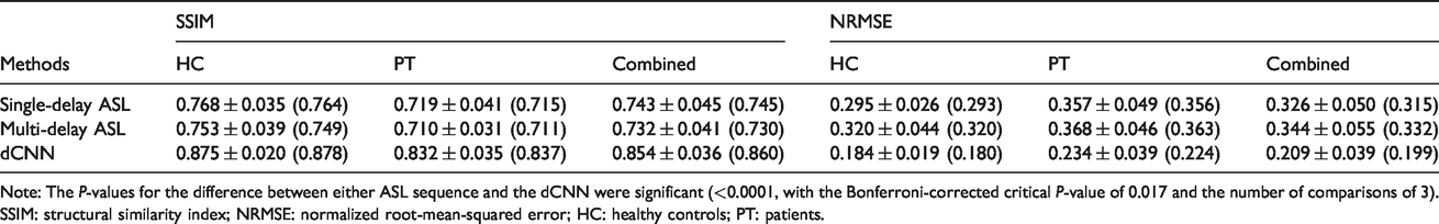
Note: The P-values for the difference between either ASL sequence and the dCNN were significant (<0.0001, with the Bonferroni-corrected critical P-value of 0.017 and the number of comparisons of 3). SSIM: structural similarity index; NRMSE: normalized root-mean-squared error; HC: healthy controls; PT: patients.

Figure 2.

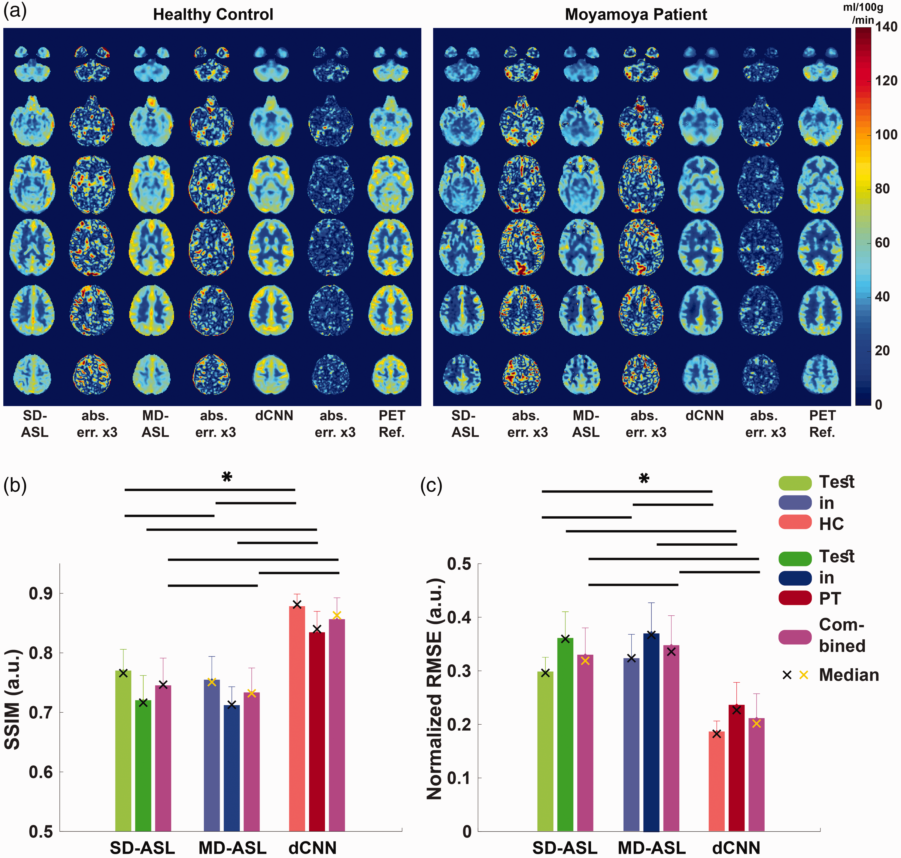
Examples of quantitative CBF maps and corresponding absolute error maps (magnified) (a) obtained using single-delay (SD), multi-delay (MD) ASL, and the deep convolutional neural network (dCNN), in a healthy control (HC) (left) and a patient with Moyamoya disease (right). Five slices across the brain are shown. Quality metrics (mean and standard deviation) of normalized CBF maps were measured by structural similarity (SSIM) (b), normalized root-mean-square error (NRMSE) (c). In b and c, light colors represent the test results in healthy controls (HC), the dark colors represent the test results in patients (PT), and the magenta represents the test results in the combined group. The cross symbols represent the median values, where yellow cross symbols indicate non-normal distribution. The dCNN showed significantly higher SSIM and lower NRMSE compared to either ASL method. Significant differences are indicated by black lines and asterisks at the top (with Bonferroni correction for multiple comparison, P < 0.0021).

CBF quantification accuracy assessment

For the normalized CBF values in all testing subjects, the dCNN showed improved correlation with PET measurements (coefficient of determination, r² = 0.488 (P < 0.001), 0.602 (P < 0.014), and 0.575 (P < 0.001) in HC, PT, and combined groups, respectively), compared with single-delay ASL (r² = 0.151, 0.439, and 0.364 in HC, PT, and combined groups, respectively) and multi-delay ASL (r² = 0.161, 0.518, and 0.405 in HC, PT, and combined groups, respectively), shown in Figure 3(a). We attribute the higher correlations in the PT group to the wider CBF dynamic range in this group.

Figure 3.

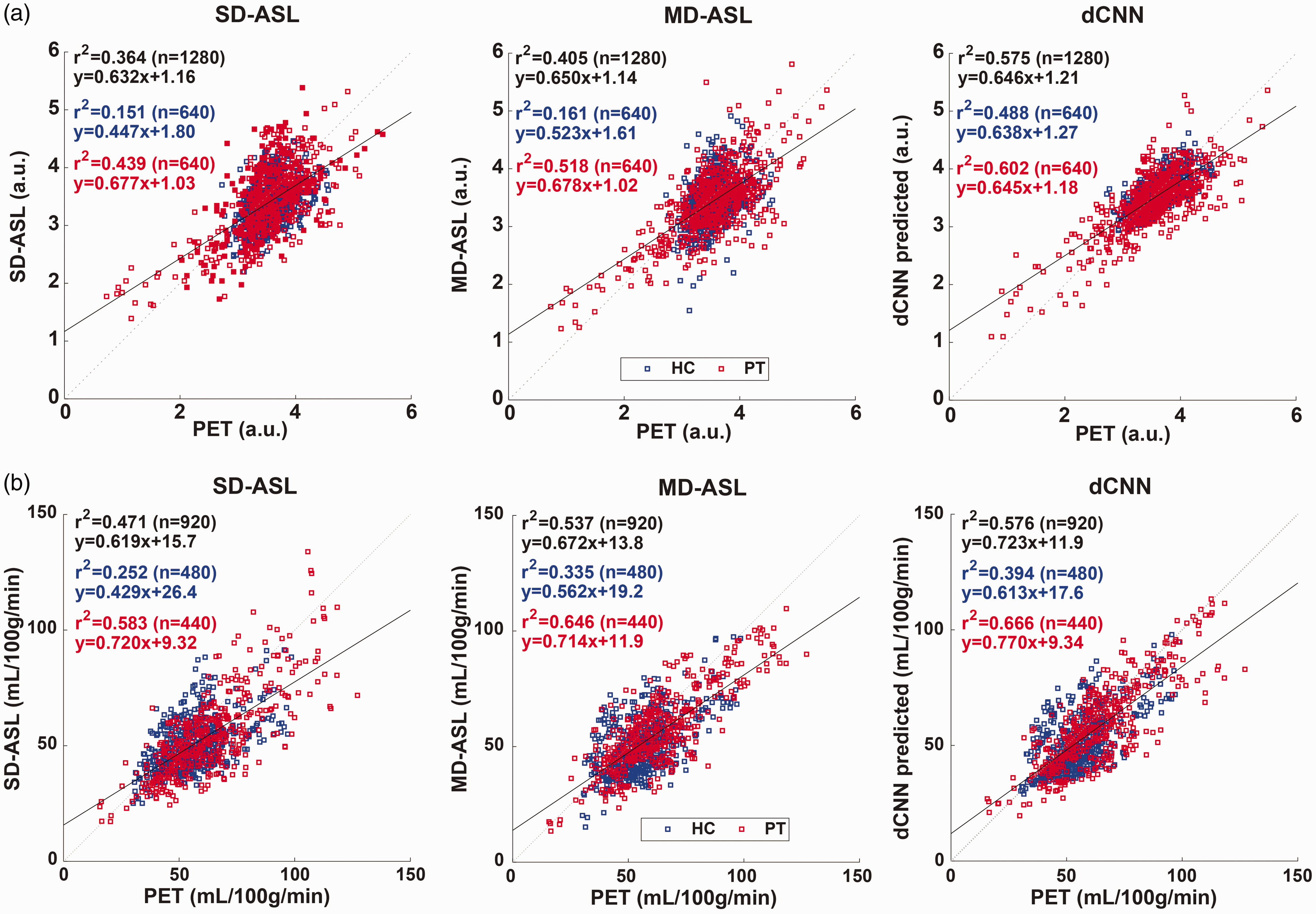
Linear regression plots of the normalized (a) and quantitative (b) mean CBF in regions of interests from single-delay (SD, left) and multi-delay (MD, middle) ASL and that produced by the deep convolutional neural network (dCNN, right). The blue and red square symbols represent the data in the healthy control (HC) and patient (PT) groups, respectively. The solid black lines and fitted parameters in black show the regression results in the combined groups (HC + PT), while the fitted parameters in the HC and PT groups are shown in blue and red, respectively. Note that a few subjects were excluded from both groups in quantitative analysis (b) due to images quality concerns (see text and Supplementary Figure S2). The dCNN showed improved correlation (in both normalized and quantitative comparisons) with measurements by PET in the HC, PT, and combined groups.

For the quantitative CBF values, the dCNN also showed improved correlation with PET measurements in HC and combined groups (r² = 0.394 (P < 0.001) and 0.576 (P < 0.001), respectively), compared with single-delay ASL (r² = 0.252 and 0.471 in and combined groups, respectively) and multi-delay ASL (r² = 0.335 and 0.537 in HC and combined groups, respectively). In the PT group, the dCNN improved correlation compared with single-delay ASL (r² = 0.666 vs. 0.583, P < 0.001), but not significantly so compared with multi-delay ASL (r² = 0.666 vs. 0.646, P = 0.039) (Figure 3(b)).

Averaging quantitative CBF values in the ASPECTS ROIs, the mean reference PET CBF (mean ± standard deviation (median)) was 56.3 ± 13.3 (55.5) and 63.0 ± 19.2 (60.6) ml/100 g/min in HC and PT groups, respectively. The dCNN model produced less biased mean CBF values of 52.1 ± 13.0 (49.7) and 57.9 ± 18.1 (55.3) ml/100 g/min in HC and PT groups, respectively, compared to single-delay ASL (50.6 ± 11.3 (48.8) and 54.7 ± 18.1 (51.9) ml/100 g/min with P < 0.0001 in HC and PT groups, respectively) and multi-delay ASL (50.8 ± 12.9 (48.4) and 56.9 ± 17.0 (54.4) ml/100 g/min with P < 0.002 in HC and PT groups, respectively). The reduced estimation error of the dCNN results is shown in the Bland–Altman plots in Supplementary Figure S3.

Examining the contribution from structural MRI input channels

The results obtained by the dCNN trained without the structural MRI input channels can be found in Supplementary Figures S4 and S5. Including the structural images as inputs to the dCNN resulted in better anatomical details, e.g. gray matter/white matter delineation, and improved regional CBF quantification compared to that without structural information. Using the anatomical channels improved SSIM and NRMSE scores (P < 0.0001), as well as improved correlation with measurements by PET in the HC group (significant, P = 0.011), although the improvement in the PT or combined groups was not significant (P > 0.097).

Examining bias of models trained on different cohorts

Examples of the CBF maps and corresponding error maps for dCNN’s trained with different cohorts (i.e. either HC, PT, or a mix of both HC and PT groups) are shown in Figure 4(a) with the averaged SSIM and NRMSE scores shown in Figure 4(b).

Figure 4.

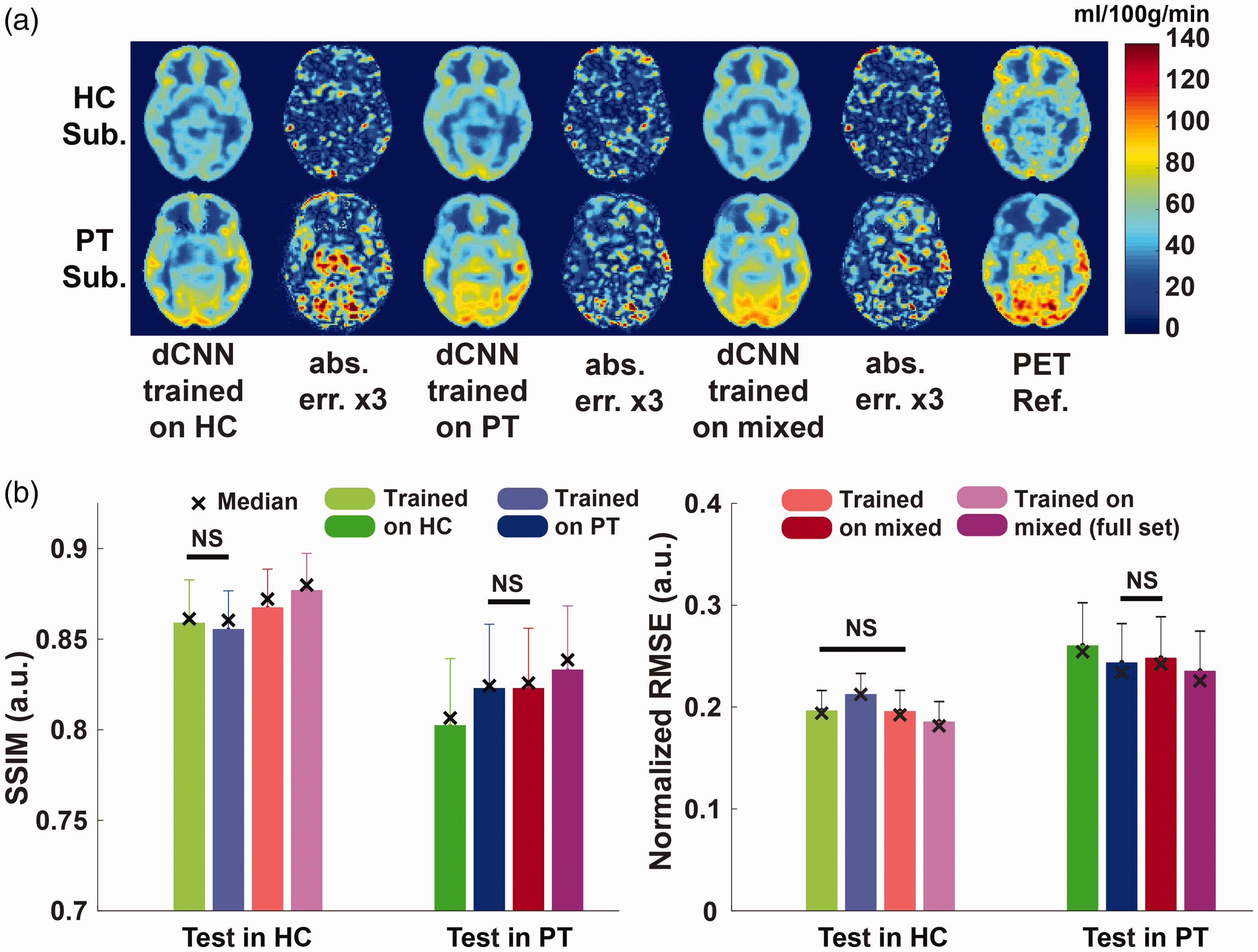
(a) Examples of CBF maps and corresponding absolute error maps (magnified) obtained using deep convolutional neural networks (dCNNs) trained on different datasets; (b) corresponding image quality metrics, structural similarity index (SSIM) and normalized root-mean-square error (NRMSE), calculated from normalized cerebral blood flow (CBF) maps. Light colors represent the test results in healthy controls (HC), and the dark colors represent the test results in patients (PT). The cross symbols indicate the median values. For comparison, the results from the dCNN trained with a larger mixed dataset (from Figure 2) are also included, shown in magenta. The non-significant comparison pairs are labeled with black lines and “NS”, while all other comparisons within the same cohort were significant (P < 0.002). With a fixed training dataset size of 24 scans, the best SSIM and NRSME scores (or non-significantly different from the best) for both test cohorts were achieved when the model was trained on a mixed cohort (red vs. green and blue). Overall, the models trained on a larger mixed cohort (full set, 48 scans) performed the best in all settings (magenta vs. all others).

Comparing the dCNN’s trained with the HC-only or PT-only group, the model trained on a specific subject group yielded better image quality on the same subject group (i.e. a model trained on HC performed best when tested on an HC cohort) than on the other groups.

When the model was trained with the mixed cohort of the same size (24 datasets), a higher SSIM (P < 0.0001) and a similar NRMSE (P = 0.34) were achieved in the HC testing datasets, compared to that trained only on HC, suggesting that replacing some HC datasets with PT datasets helped improve the dCNN’s performance in the HC group. However, similar trend was not observed when testing in PT, i.e. the model trained on the mixed cohort did not yield improved SSIM (P = 0.90) or NRMSE (P = 0.020) compared with that trained only on PT. Given the same training data size, the model trained on the mixed cohort produced overall the best image quality.

Finally, training on a mixed cohort with a doubled data size (the model trained originally with 48 datasets) improved the dCNN’s performance further on both the SSIM (P < 0.0001) and NRMSE scores (P < 0.0001) in both HC and PT groups. This demonstrated that the dCNN’s performance improved upon increased training data size with a mixed cohort. In addition, when compared with the dCNNs trained on HC or PT groups only (24 datasets each), adding (rather than substituting) datasets from the other group improved the SSIM and NRMSE scores in testing in HC or PT groups (P < 0.0001, Figure 4(b)).

Results on the correlation of the mean normalized CBF from PET and from dCNNs trained on different cohorts are summarized in Table 3. Comparing the dCNNs trained on different cohorts of the same size, the dCNNs produced higher correlation in the corresponding group that they were originally trained on (P < 0.001). For instance, the dCNN trained on a mixed cohort yielded moderate correlation coefficients in HC- or PT-only cohorts, but gave highest correlation coefficient in the mixed cohort (significantly greater compared with PT-only, P < 0.001; but not significantly when compared with HC-only, P = 0.022). Training with the larger, full mixed datasets produced the highest correlation coefficients in the HC (though not significantly when compared with those trained HC-only or smaller mixed groups, P > 0.445) and mixed (significantly, P < 0.007) groups.

Table 3.

Fitting results of normalized cerebral blood flow values in the regions of interest using deep convolutional neural networks trained on different cohorts.

Testing dataset	Healthy Controls		Patients		Combined
	r2	β	r2	β	r2	β
Trained on HC (24)	0.451	0.618	0.540	0.465	0.485	0.499
Trained on PT (24)	0.306	0.663	0.661	0.700	0.540	0.698
Trained on mixed (24)	0.432	0.587	0.594	0.646	0.552	0.639
Trained on mixed (full set, 48)	0.488	0.638	0.602	0.645	0.575	0.646

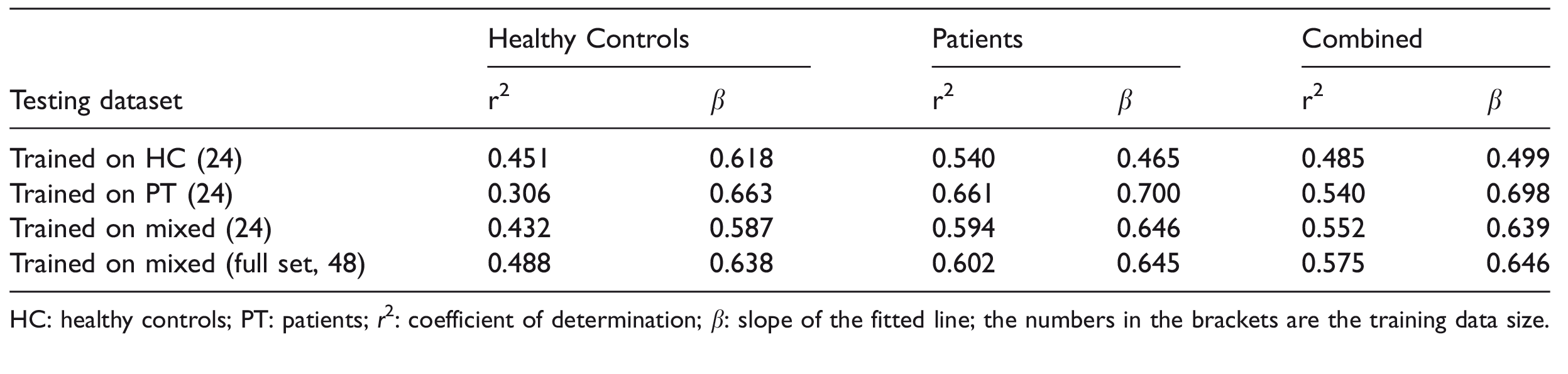
HC: healthy controls; PT: patients; r²: coefficient of determination; β: slope of the fitted line; the numbers in the brackets are the training data size.

Discussion

We developed a dCNN-based model to integrate information from multiple MRI contrasts, including two ASL scans, to predict CBF maps with significantly improved image quality and quantification accuracy than either ASL measurement alone, using simultaneously acquired PET CBF measurements as the reference. We also examined the bias effect of using different training cohorts on the performance of the dCNN, and showed that training on the complete dataset including both HC and PT yielded overall the best outcome in both groups.

Comparing the CBF maps from the original ASL and PET scans, regional structural differences can be observed. These are likely due to imaging modality differences, spatial resolution differences, imperfections in the image reconstruction and co-registration processes, as well as regionally varying inaccuracies due to arterial arrival time. These differences contribute to the lower SSIM and higher NRMSE scores for the original ASL measurements. One consistent finding was that both ASL methods underestimated CBF in the basal ganglia, likely due to early ATT and subsequent T₁ decay within the tissue compartment; this error was learned by the deep network and corrected on the synthesized CBF maps. In addition, the contrast around infarcts improved in general, while the residual arterial artifacts presented in ASL were reduced (Supplementary Figure S1). The dCNN was able to match the structure of the PET images, with improved SSIM and NRMSE metrics; more importantly, it yielded more accurate CBF estimates, which is clinically relevant.

ASL scans with insufficiently long PLDs are likely to underestimate perfusion if the flow is delayed due to disease, as in the cerebrovascular patients. With a wider PLD range to cover these prolonged ATTs, the perfusion quantification accuracy can be improved, as shown by the multi-delay ASL measurements. By integrating information from multiple contrast sources, including the CBF and the ATT maps from single-delay and multi-delay ASL scans as well as structural scans, the dCNN further improves the quantification accuracy. Examples in Supplementary Figure S1 show that some of the typical defects in the CBF distribution in the ASL methods due to transit delay effects, e.g. the frontal lobes and watershed areas, were compensated for in both HC and PT cohorts. Another example is the correction for the spurious defects in the left frontal area in HC #1 that presented in multi-delay ASL but not in single-delay ASL due to acquisition error.

We observed that some of the quantitative PET CBF maps might have quantification errors when an IDIF was not accurately generated, which were likely to be globally scaled incorrectly. By using normalized CBF maps, the dCNN models can learn the regional flow information without being affected by potential quantification errors introduced by global scaling in the PET reference images. Consequently, including all the subjects in the analysis on normalized, instead of quantitative, CBF measurements should be more appropriate. However, other factors that affect the accuracy of the regional flow distribution in the PET reference images, e.g. imperfect single-atlas based attenuation correction, may still be presented and affect the analysis. Recent development, such as multi-atlas-based method, ⁴² zero-TE imaging, ⁴³ etc., should be able to improve the attenuation correction and provide a better reference. On the other hand, we excluded subjects with likely PET quantification errors to accurately analyze the quantitative CBF values. The exclusions should not bias the final results between single-delay, multi-delay ASL and dCNN, as the exclusion criteria were based on the average of the three.

In this study, simple gray matter masks based on the gray matter probability were applied in the ROI analysis. A relatively high threshold (0.8) was used to help reduce the CBF estimation inaccuracy from white matter which could come from two sources: (1) varying white matter probability within the ROI; (2) the uncertainty in white matter CBF quantification in ASL as only gray matter T₁ was used. The quantification accuracy could be improved by partial volume correction methods, such as ⁴⁴ for ASL and ⁴⁵ for PET, which should be included in the future work.

The improvement on the image quality and normalized CBF prediction accuracy when structural channels were included as inputs, demonstrated their important contribution in the prediction task. In addition to the structural information itself, e.g. shape, boundary, etc., the structural input channels may help provide information on CBF quantification by serving some regularization purpose, as the CBF values are tissue type dependent. However, there may be potential risk of mixing physiological and anatomical information in an undesired way and result in compromised performance, especially in patient populations where mismatch between physiological and anatomical information is more likely to occur. In this study, the additional convolution path introduced to the U-Net structure was used to emphasize perfusion-related information and reduce the afore-mentioned risk, resulting in improved performance. In addition, training of a dCNN model using only the structural images as input yielded poor results, especially those from the regression analysis in the PT cohort, demonstrating the essential importance of perfusion information in this prediction task (please see Supplementary Figure S6).

Comparing the dCNNs trained with different cohorts for model bias assessment, the overall best performance was observed when the composition of the training cohorts (HC-only, PT-only and mixed) matched that in the testing. Adding/replacing some PT datasets in the HC training datasets improved the dCNN’s test performance in the HC group, demonstrated by improved SSIM, NRMSE, and correlation coefficients; however, adding/replacing some HC datasets in the PT datasets did not show such benefit. It is likely that the higher regional CBF variation in PT datasets due to the presence of disease, in addition to “healthy regions”, made the dCNN model more robust for predicting CBF in the HC group. This indicates the high value of training on PT data; however, these datasets are also relatively more difficult to acquire compared to HC datasets. Generally, without a priori knowledge on whether a subject has cerebrovascular disease or not, a model trained with a mixed cohort is recommended; in addition, it should be beneficial to include as many subjects in the training cohort as possible.

The total number of original input images (62,720) was sufficiently large, despite the limited number of subjects. Data augmentation further increased this by three-fold. The data augmentation step in the training, although very simple (i.e., only flipping and transposing), significantly improved the performance (please see Supplementary Figure S7 for the comparison to the dCNN trained without augmentation), demonstrating its importance. Though data augmentation increases the training time by a few folds (about 3 folds in this study), the prediction (application of the models) time remains the same once the model is trained. In each cross-validation step, 75% of these images were used in training. In all the studied scenarios, we relied on cross-validation and monitoring of the training/validation loss during training for each training step to assess whether the networks were over-fitting, and none was observed. In addition, the good performance on the test datasets in all the tested scenarios also suggested that over-fitting did not occur in this study.

Despite the promising improvements using the dCNN, there are still minor discrepancies between the synthesized and reference PET CBF maps, e.g. the overestimation of CBF in the infarct area in PT #4 (Supplementary Figure S1). The performance of the dCNN should be further improved by including more training data, especially those from the PT group, as suggested by the trend shown in this study. In addition, it should also be beneficial to include ASL scans that are less sensitive to transit delay effects, e.g. ASL scans with longer LD and PLD, ⁸ or velocity-selective ASL.^12–14 Note that the SNR efficiency of the single-delay ASL in the current study was suboptimal (91.1% of that if a recommended LD of 1.8 s is used ⁶ ) due to a short LD of 1.45 s, and could be improved by using a longer LD.

Currently, the dCNN takes all the input contrasts, which may contain redundant information, or may not be readily generalizable due to images acquired with specific scan parameters, e.g. the individual ASL signal at five specified PLDs. An optimized combination of the input contrasts would be desired to simplify and generalize the pipeline. This optimization may benefit applications in datasets that include both single-delay and multi-delay ASL measurements but were acquired with different imaging parameters or on different scanners, e.g. the ADNI dataset. As part of the optimization process, the dCNN trained with only single- or multi-delay ASL (with structural images) was also evaluated. The results (please see Supplementary Figure S8 for details) showed that while including both single- and multi-delay ASL in the training gave the best results as expected, it is interesting that the dCNNs performed reasonably well with only single-delay or multi-delay ASL data, demonstrating significant improvement compared to the original ASL scans. This is especially encouraging as the majority of clinical sites will at most acquire one ASL scan, which may benefit from the proposed dCNN method. On the other hand, it may be also worth to optimize imaging parameters and/or protocol to allow more than one type of ASL scans in a scan session within similar total scan time to obtain additional improvement. A U-net structure with skip connection and absolute error as the cost function was used in this study. It is worth exploring other network structures and/or cost functions for performance improvement, e.g. recently proposed general adversarial networks (GANs). ⁴⁶

This study focused on the Moyamoya disease despite its relative rarity, as these patients often show severely prolonged transit delays that pose large challenges in perfusion quantification with ASL. With promising results in this patient population, we may expect better performance in other vascular diseases and dementia where similar but less severe vascular alterations are present. Our results in the atherosclerotic steno-occlusive disease patients included here suggested a trend of better performance (data not shown) though the number of patients was small.

The data in this study included the CBF maps acquired before and after hemodynamic challenge, so cerebral vascular reactivity maps can be calculated. With improvement on the perfusion quantification in both pre- and post-challenge conditions, one would expect improvement on reactivity maps, especially within the areas where the transit sensitivity of ASL may exaggerate the reactivity response, though this has to be studied to confirm. However, exploiting the reactivity maps was not within the scope of the current study and will be examined in future work.

This study had several limitations. First, to minimize patient discomfort, arterial blood samples were not collected, so the PET CBF maps were generated based on an IDIF method, ²⁴ which is sensitive to errors from PET image reconstruction and vessel segmentation errors. To improve the quality of the reference “ground truth”, arterial blood samples could be collected. An alternative approach is to scale the whole brain CBF by another measurement, e.g. the whole brain flow measured by phase-contrast imaging.^47,48 However, scaling methods should be used cautiously, as systematic bias has been shown between phase-contrast MRI and ¹⁵O-water PET with arterial sampling,^43,49 especially at lower spatial resolutions and for higher flow rates. Furthermore, the validity of phase-contrast MRI in patients with steno-occlusive disorders is less well understood. In these patients, slower flow may lead to reduced SNR and contributions from compensatory collateral arteries (e.g. via the extracranial vessels) may not be properly measured. Second, the final predicted CBF maps were scaled by the mean CBF from the multi-delay ASL, and could be affected by factors such as labeling efficiency. To mitigate this, other flow measurements, such as phase-contrast or pulsed ASL, which has high and constant labeling efficiency, can be included to help improve the quantification accuracy of the dCNN model. Third, the number of subjects was limited due to data availability, affecting both the training process and the testing validation. The dCNN is expected to have improved performance with bigger datasets, though it performs well with the limited number available for this study. In addition, only limited cerebrovascular disease types were included in this study, mainly Moyamoya disease and steno-occlusive disease of the carotid arteries. Therefore, whether the performance of the current dCNN model can generalize in other cerebrovascular or neurodegenerative diseases remains to be evaluated. Furthermore, due to the availability of such datasets, the performance of the dCNN on ASL measurements across different scanners or vendors was not examined in the current study. The current dCNN model is implemented in 2 D. A 3 D implementation would be more appropriate to integrate the information along the slice direction, potentially improving its performance. Lastly, relatively simplistic statistical methods were used in comparing the performance of the dCNN models and ASL measurements, and possible within-subject correlations (e.g. correlation between adjacent slices, between the two measurement runs) were not examined and might affect the accuracy of the performance comparisons.

To conclude, we demonstrated that the proposed dCNN is capable of integrating multi-contrast information from ASL and structural MRI to synthesize CBF maps with significantly improved image quality and quantification accuracy, in both healthy subjects and cerebrovascular disease patients. We also showed that training on patient data improves performance, as it contains valuable information about both healthy and diseased regions. Using a dCNN should allow more accurate CBF measurements in patients who receive only MRI and do not have access or capability to undergo ¹⁵O-water PET CBF mapping.

Supplemental Material

JCB888123 Supplementary material - Supplemental material for Predicting ¹⁵O-Water PET cerebral blood flow maps from multi-contrast MRI using a deep convolutional neural network with evaluation of training cohort bias

Supplemental material, JCB888123 Supplementary material for Predicting ¹⁵O-Water PET cerebral blood flow maps from multi-contrast MRI using a deep convolutional neural network with evaluation of training cohort bias by Jia Guo, Enhao Gong, Audrey P Fan, Maged Goubran, Mohammad M Khalighi and Greg Zaharchuk in Journal of Cerebral Blood Flow & Metabolism