The resting-state fMRI arterial signal predicts differential blood transit time through the brain

Abstract

Previous studies have found that aperiodic, systemic low-frequency oscillations (sLFOs) are present in blood-oxygen-level-dependent (BOLD) data. These signals are in the same low frequency band as the “resting state” signal; however, they are distinct signals which represent non-neuronal, physiological oscillations. The same sLFOs are found in the periphery (i.e. finger tips) as changes in oxy/deoxy-hemoglobin concentration using concurrent near-infrared spectroscopy. Together, this evidence points toward an extra-cerebral origin of these sLFOs. If this is the case, it is expected that these sLFO signals would be found in the carotid arteries with time delays that precede the signals found in the brain. To test this hypothesis, we employed the publicly available MyConnectome dataset (a two-year longitudinal study of a single subject) to extract the sLFOs in the internal carotid arteries (ICAs) with the help of the T1/T2-weighted images. Significant, but negative, correlations were found between the LFO BOLD signals from the ICAs and (1) the global signal (GS), (2) the superior sagittal sinus, and (3) the jugulars. We found the consistent time delays between the sLFO signals from ICAs, GS and veins which coincide with the blood transit time through the cerebral vascular tree.

Introduction

Blood-oxygen-level dependent (BOLD) contrast is primarily used in functional MRI (fMRI) to detect brain activation.^1,2 This technique relies on the fact that deoxy-hemoglobin is paramagnetic, which causes MR signal to decrease in T₂*-weighted images. Therefore, the BOLD contrast depends on the amount of deoxy-hemoglobin in a voxel. The connection between the brain activation and BOLD contrast is through neurovascular coupling. In detail, regional brain activation (neuronal firing) increases the local metabolic rate, which increases the blood flow and volume to bring in more oxygen and nutrients to the site. This leads to an oversupply of oxygenated blood due to the “uncoupling of oxidative metabolism”; ³ the resulting increase in oxy-hemoglobin concentration and decrease in deoxy-hemoglobin concentration leads to a local increase in T2*, and an increase in the BOLD signal intensity. Thus, BOLD signal is not a direct measurement of the brain activation, but rather a measure of hemodynamic changes resulting from neuronal activation. ⁴ However, many other physiological processes, which change the blood flow, oxygenation and volume, also induce BOLD signal changes. ⁵ Cardiac pulsation and respiration signals, or more usually, aliased versions of these signals, are also visible in BOLD fMRI data.^6–9 In addition, there are low frequency variations in the BOLD signal of unknown origin, collectively known as “low-frequency oscillations.” ⁹

One of these low frequency contributions to BOLD variance is called “systemic low frequency oscillation” (sLFO: ∼0.1 Hz). ¹⁰ Different from other low-frequency oscillations in BOLD, sLFO signals are likely non-neuronal and widely observed in the brain by fMRI. In this paper, we will use this term (sLFO) to distinguish this signal from resting state LFO BOLD signals, which arise from neuronal activity changes. It has previously been demonstrated that this sLFO, estimated from the global signal (GS) of the BOLD signal in resting state fMRI data, can be used to track cerebral blood flow throughout the brain by determining the time lags between the sLFO and the BOLD signals from different voxels.^11–14 This indicates that the sLFO is closely associated with dynamic blood flow, thus travels with it to different parts of the brain. These sLFOs can also be detected throughout the periphery. For example, they are found in fingertips and toes using near-infrared spectroscopy^15,16 as changes in oxy-hemoglobin concentration. The sLFOs recorded at the fingertips lead those from the toes by about 3 s, and both are highly correlated with the GS of resting state fMRI which were acquired simultaneously. The BOLD signal arises both from changes in blood volume and blood oxygenation. Oxy-hemoglobin concentration is a good proxy for blood volume changes in arterial blood, since arterial blood is essentially 100% oxygenated. If this is the case, the sLFO signals seen in the periphery, and throughout the capillaries and veins in resting state fMRI data, should be observable in the BOLD signal of the cerebral arteries. Furthermore, the sLFO signal in the arteries should lead the signal found in the capillaries and veins (sequential arrival times). To date, we are not aware of any effort to search for this sLFO signal in the arteries using fMRI. In this study, we looked for the sLFO BOLD signal in the arteries (i.e. internal carotid artery, ICA) and compared it to the GS, which reflects primarily the capillary and venous blood, and to the signals found in prominent veins (e.g. superior sagittal sinus, SSS and internal jugular vein, IJV). We hypothesized that the sLFO BOLD signals would be detected in all these compartments (as indicated by significant cross-correlation between these signals and the GS, and with each other), and that the relative delay times will be consistent with the flow of blood from arteries, through capillaries, to veins. This study seeks to test these hypotheses. Since the contrast mechanisms generating the signals from large arterial vessels are not clear, we will still refer to them as “BOLD signal”. Details can be found in the discussion.

Materials and methods

Ethical statement

The request of re-analyzation of publicly available data was submitted to Purdue University Institutional Review Board (IRB) office, which determined that it did not meet the requirements for human subject research, and thus that IRB approval was not necessary.

Myconnectome

To test the hypothesis, we used the publicly available Myconnectome dataset (http://myconnectome.org/wp/). Myconnectome is the most thorough publicly released imaging study of a single person. ¹⁷ We analyzed 90 resting state scans collected over the duration of two years on this subject. The Myconnectome dataset has several features making it particularly suited to this study: (1) Since there are 90 resting state scans from a single subject, this made it easy to assess the reliability of the results with little within-subject variation. (2) The simplified registration procedure due to all images belonging to the same subject minimized alignment errors; this is critical in mapping arteries in resting state data with low signal-to-noise ratio (SNR); (3) Myconnectome's multiband resting state acquisitions are high quality data with relatively high temporal (TR = 1.16 s) and spatial resolution (∼2.5 mm³); (4) The anatomic data include repeated T1 and T2-weighted scans with high spatial resolution, which allows us to accurately identify large vessels (arteries and veins); (5) Myconnectome’s structural and functional data cover the full extent of the head and a significant portion of the neck, which allows a relatively large fraction of the ICAs to be identified; (6) The data are publicly available, which allows these results to be independently verified (our methods, software, and results will be available online). The detailed scan parameters have been described previously. ¹⁷ Briefly, most of the fMRI scans use a multi-band EPI sequence (TR = 1.16 s, TE = 30 ms, flip angle = 63°, voxel size = 2.4 × 2.4 × 2.0 mm, distance factor = 20%, 68 slices, oriented 30° towards the coronal plane from the AC-PC line, 96 × 96 matrix, 230 mm FOV, MB factor = 4, 10:00 scan length).

Preprocessing

Ninety resting state scans from Myconnectome were preprocessed using FSL (FMRIB Expert Analysis Tool, v5.98, http://www.fmrib.ox.ac.uk/fsl, Oxford University, UK). ¹⁸ Preprocessing steps include: (1) motion correction; (2) brain extraction; (3) registration to the T1-weighted image. The GS was calculated from each resting state dataset after brain extraction.

Artery and vein extraction

We identified the left and right ICAs and IJV, and the SSS from the T1 and T2-weighted scans. The left and right ICAs are clearly visible in the T1-weighted anatomic scans (Figure 1(a)) due to the enhancement of inflowing blood in gradient echo T1-weighted scans. On the other hand, the large veins are not easily identifiable in either T1- or T2-weighted images. However, the contrast of signals in large blood vessels is increased in the image by using the ratio between the T1- and T2-weighted images. ¹⁹ As shown in Figure 1(b), ICAs, SSS and IJVs are all bright in the ratio image. By carefully thresholding the image, we can extract ICAs, SSS and IJVs with great accuracy (Figure 1(c)).

Figure 1.

The flowchart of the processing procedure is shown. From averaged T1w image of the subject (a) and the averaged image of T1w divided by T2w (b), left and right internal carotid arteries (L-ICA, R-ICA), superior sagittal sinus (SSS), left and right internal jugular veins (L-IJV and R-IJV) were distinguishable (indicated by the arrows in (b) and (c)). The projections of these vessels on one example of low-resolution resting-state fMRI image (d). These vessel projections are used as masks to extract the corresponding averaged time series (TS) from each resting state scan, i.e. left ICA, right ICA, SSS, left IJV and right IJV. The time series were filtered at range of 0.005–0.1 Hz to remove high-frequency noise and signal drift. Lastly, the correlation coefficients and time delays were calculated between each time series and the global signal.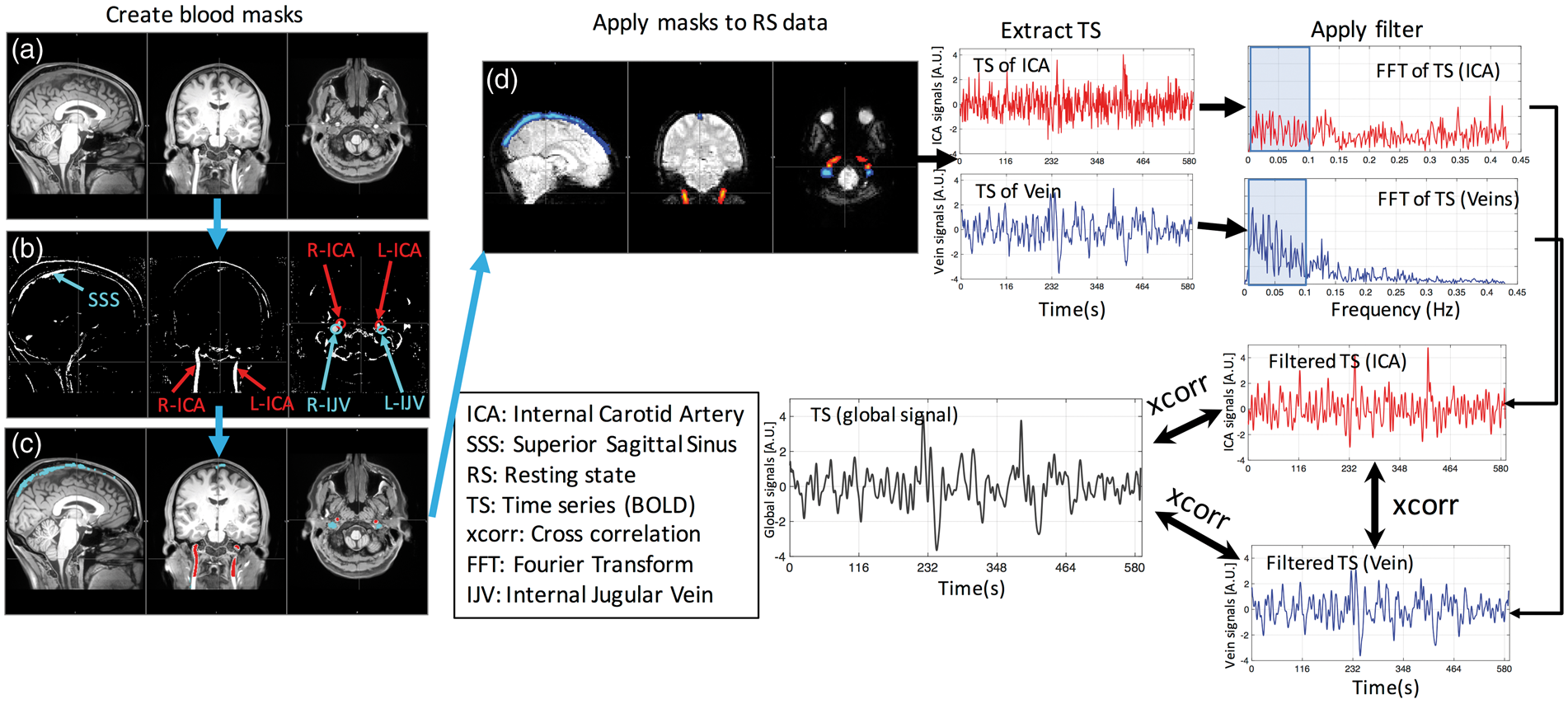

Correlations and delays

Figure 1 shows the flowchart of the analyses.

Using the procedures outlined previously, five vessels were identified (the left and right ICA, the SSS and left and right IJV). For each resting-state scan, these high-resolution vessel images were registered to the low-resolution functional images using the registration matrix calculated in the preprocessing steps. One example of the registrations is shown in Figure 1(d). The five registered vessel images were then used as masks to extract the corresponding time courses for each blood vessel. As we can see in Figure 1(c), the ICAs and IJVs are clearly separable (no-overlap) in the high-resolution images. However, when we registered them onto the low-resolution resting state image, the boundaries of these vessels (ICA and IJV) may overlap (Figure 1(d)). When these registered images were used as masks to extract corresponding time series, we used weighted average option in the FSL function (fslmeants –w) to minimize the registration error, especially in those overlapping boundary voxels. Weighted averaging is also applied to extract BOLD signals from SSS.

A band-pass filter (0.005–0.1 Hz) was applied to these time courses to obtain the low-frequency BOLD signals. Finally, cross correlations were performed to calculate the maximum cross correlation coefficients (MCCCs) and the corresponding time delays between the sLFO BOLD signals of: (1) left ICA; (2) right ICA; (3) the GS, (4) the SSS, (5) left IJV and (6) right IJV. The correlation peak search window was set to be ±15 s, as the total transit time of blood through the head is less than 10 s in healthy subjects. ²⁰ Here, when determining the MCCC, we also consider the negative correlation values (i.e. MCCC is then the maximum absolute value of the cross-correlation coefficient). NOTE: Because the sLFO signals are in general aperiodic, they have no “phase”, only time delay, so a negative correlation happens at a specific time delay only if the signal is inverted, rather than being “180 degrees out of phase”. Details can be found in “Effects from cross correlation” of discussion.

Lastly, significance may be overestimated when processing steps such as bandpass filtering and optimal delay search are used. ²¹ To assess the spurious correlation threshold (above which correlations would be considered significant) in this study, we conducted the so-called “mismatch” cross-correlation calculations. For example, to assess the spurious correlation level between the ICA and GS, we intentionally selected ICA and GS from different sessions, which should be uncorrelated. By keeping the rest of the processing procedure the same (e.g. filtering, correlation, and peak selection), we can calculate the distribution of spurious correlations in MCCCs and corresponding time delays. Moreover, we employed the two sample Kolmogorov–Smirnov test to see if the distributions of MCCCs and time delays from the actual calculations are significantly different from those from the “mismatch” calculations.

Results

Figure 2 shows sample BOLD signals corresponding to the GS, the right ICA, the SSS and right IJV, taken from one resting state scan session (prior to filtering). The corresponding Fourier transforms (FTs) of these fMRI time courses are shown in the right panel. The GS, SSS and IJV BOLD signals appear quite similar, which is confirmed by their overlapping frequency distributions in the low frequency range, as seen in the FT graphs (right panel in Figure 2(b) and (c)). The ICA time courses, in contrast, have more high frequency content in their signals than those of the veins, as seen in the FT graphs. From Figure 2(b) and (d), we can also observe relative high-frequency oscillations around 0.15 Hz. This is also observed in supplemental material (SM) Figure A.2., which shows the time series and FT of the motion parameters from the same resting state session. These observations suggest that respiration may be the source of these higher frequency components. In this study, we chose the bandpass filter range as 0.005–0.1 Hz to avoid the effects of respiration in our signals.

Figure 2.

Example time series (TS) (and their corresponding Fourier transforms (FT)) of the (a) global signal (GS), (b) superior sagittal sinus (SSS) BOLD signal, (c) right internal jugular vein (R-IJV) BOLD signal, and (d) right internal carotid artery (R-ICA) BOLD signal. In the FT’s, the shaded line represents the FT of the GS, and the shaded area represents the range of the bandpass filter.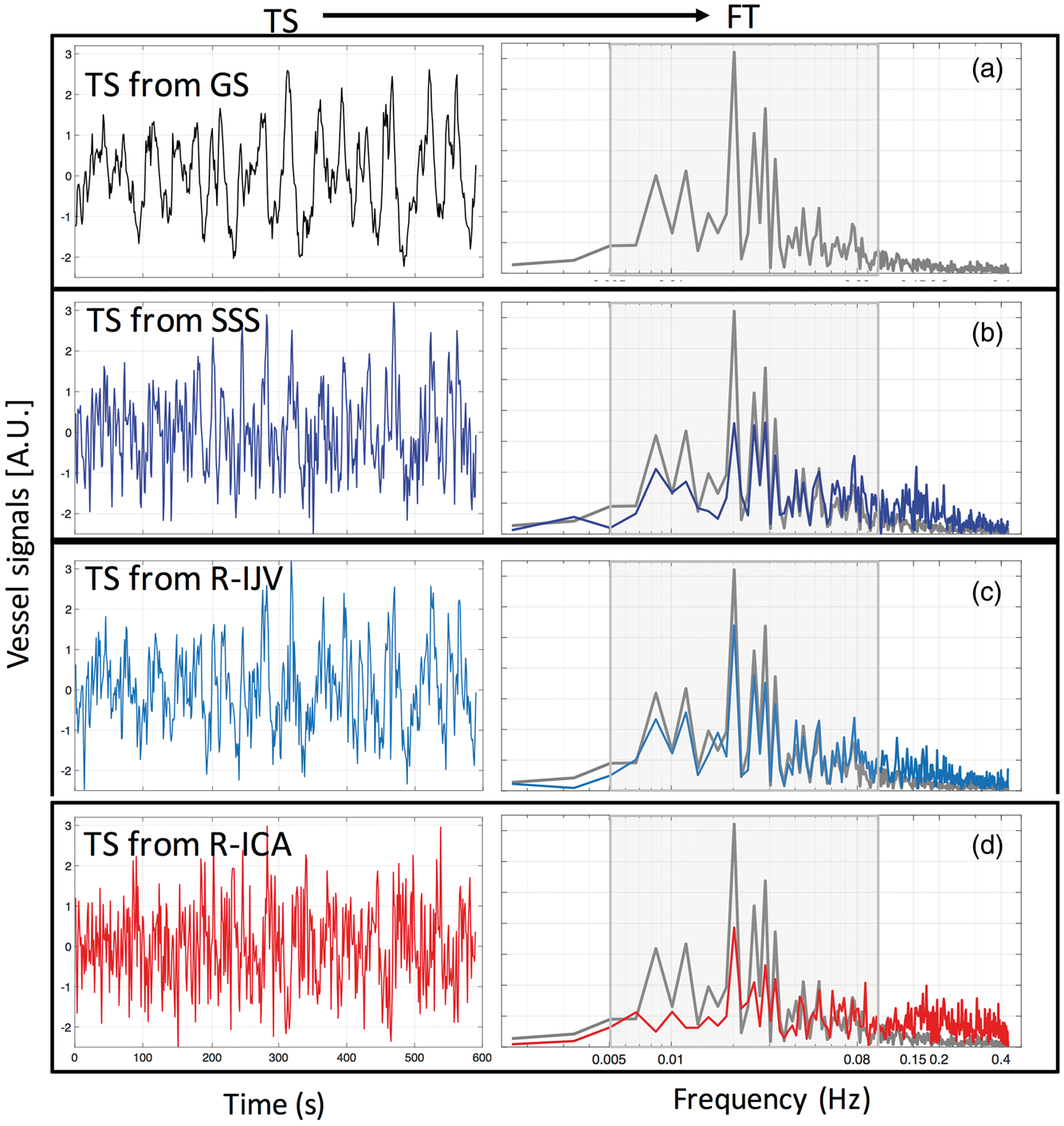

The example BOLD signals (Figure 2) are shown in Figure 3 after filtering. The BOLD signal from the ICA was inverted (multiplied by −1) when compared to the GS (since the MCCC is negative) in Figure 3(a) for clarity. The MCCCs and corresponding time delays are also listed. Here, a negative value of time delay indicates that the BOLD signal in the ICA is ahead of (leads) the GS. The shaded lines in the graphs (a, c and d) represent the GS, while the red, blue and light blue lines (in a, c and d) represent the BOLD signals of the right ICA (inverted), SSS and right IJV, respectively. Figure 3(b) shows the cross-correlation function (correlation coefficient vs. time delay) between the right ICA BOLD signals and the GS. The top panel shows the full correlation function (time delays from −600 to +600 s), while the lower panel shows the search window of −15 s to +15 s. We can see that the negative correlation coefficient is not the result of spurious correlation since its value is significantly larger (∼−0.8) than the neighboring positive peak values (∼0.4). Moreover, as seen in Figure 3(b), the general results of this study do not depend on correlation window selection.

Figure 3.

Comparison of example filtered fMRI time courses between the global signal (GS) (shaded line) and right ICA (R-ICA: red) in (a) GS and SSS (blue) in (c), GS and right IJV (R-IJV: light blue) in (d). To show the negative correlation more clearly in the figure, the R-ICA time series has been inverted (multiplied by −1) in (a). The full cross correlation between the ICA BOLD signals and GS of (a) is shown in (b) with full temporal range (top) and partial temporal range (bottom). The maximum cross-correlation coefficient (MCCC) and corresponding time delays (ΔT) calculated between fMRI of each vessel type and GS are shown in each graph (a,c,d). Positive ΔT means the GS is leading the other signal.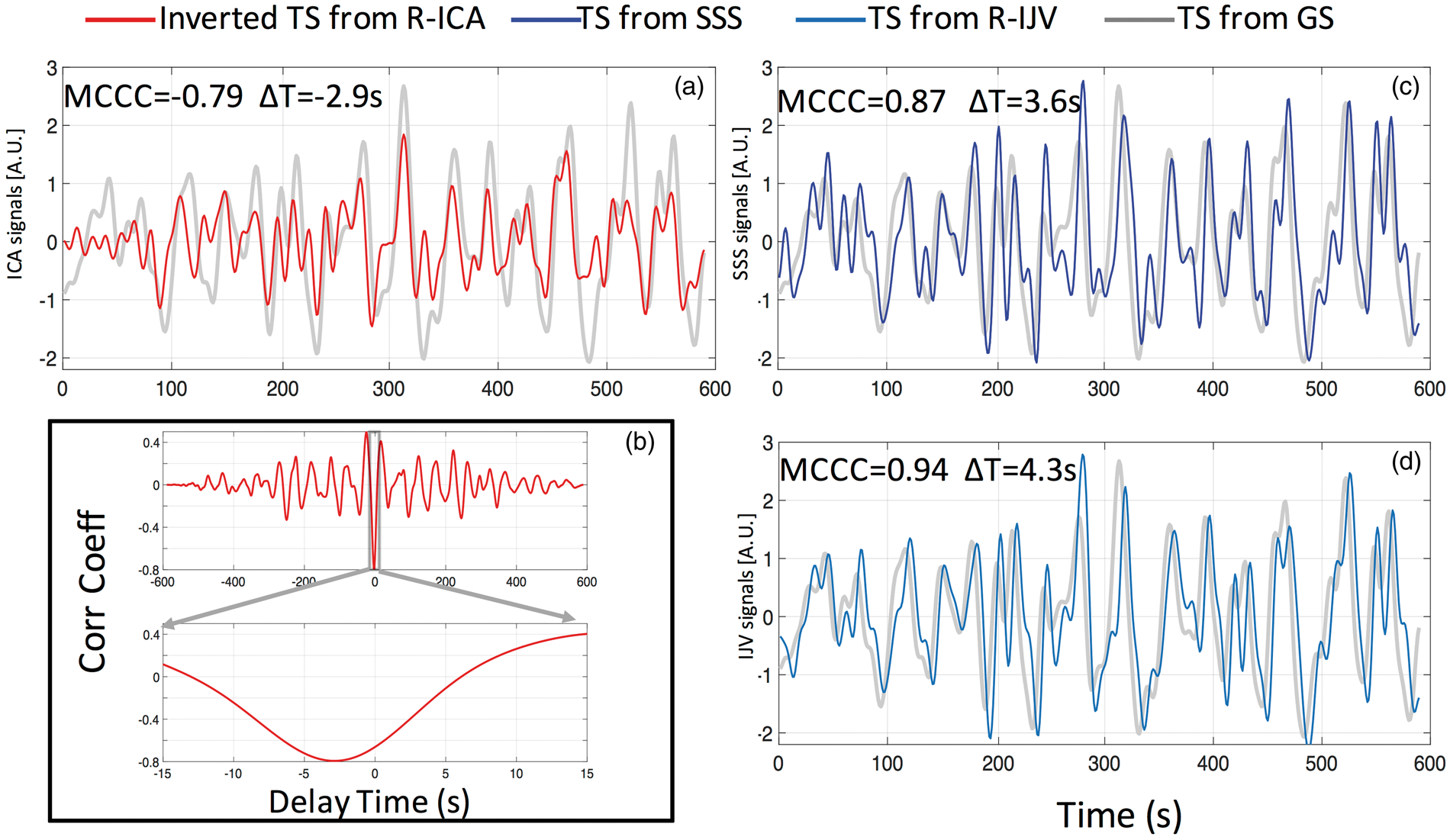

In Figure 3, we see for this resting state session, the GS and the SSS and right IJV sLFO BOLD signals are strongly and positively correlated (MCCC = 0.87, 0.94), and the GS and the right ICA sLFO BOLD signal are negatively correlated (MCCC = −0.79). The ICA sLFO BOLD signal leads the GS by 2.9 s, while the SSS and right IJV sLFO BOLD signals lag the GS by 3.6 s and 4.3 s, respectively.

Figure 4 shows the peak cross-correlation values (a) and corresponding time delays (b) calculated from 90 resting state scan sessions: (1) between GS and SSS (blue), (2) between GS, left ICA (orange) and right ICA in (red). For the GS and SSS sLFO BOLD signal, the MCCC (0. $81\pm$ 0.10) and time delay (3.2 $2\pm$ 0.59 s) were highly consistent for 88 out of 90 sessions, as seen in the distribution graphs on the right. This is because the same sLFO BOLD signals dominate both the GS and SSS, as shown in Figures 2 and 3. This result is consistent with previous observations by other groups. ²²

Figure 4.

(a) Maximum cross-correlation coefficient (MCCC) calculated from 90 resting state scan sessions, between the global signal (GS) and: SSS (blue), left ICA (L-ICA: orange) and right ICA (R-ICA: red). The distributions of these MCCCs (between −1 and 1) are shown in the graph on the right with matching colors. The 90 time delays corresponding to MCCCs in (a) are shown in (b) with the corresponding distribution histogram on the right. The averaged MCCCs and time delays were calculated. For ICAs, the positive MCCC and delay times were excluded from calculation of the average.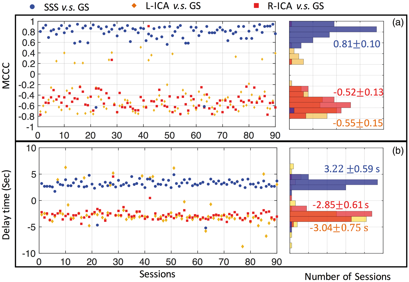

For the GS and ICA sLFO BOLD signals, in 77/88 out of 90 sessions, we obtained consistent negative MCCCs (−0. $52\pm$ 0.13 and −0. $55\pm$ 0.15) and time delays (− $2.85\pm$ 0.61 s and −3. $04\pm$ 0.75 s) for the left and right ICAs, respectively. The positive values of MCCC and time delays are excluded from the calculation of the average. However, those excluded points are not necessarily all from spurious correlation. Details can be found in “Effects from cross correlation” of discussion. As in Figure 3, the positive delay value means the GS leads the other signal.

To assess the effect of spurious correlations, we compare the distribution of the simulated null distribution (MCCC and time delay) obtained from the “mismatch” correlations between: (1) left ICA and GS (a); (2) right ICA and GS (b); SSS and GS (c) in Figure 5 with the distribution of real data (previously seen in Figure 4). The “real” distributions are all significantly (p < 0.0001) different from the noise baseline.

Figure 5.

Distribution of MCCCs (left) and corresponding time delays (right) calculated from 90 resting state scan sessions, between global signal (GS) and: left ICA (L-ICA: orange in (a)), right ICA (R-ICA: red in (b)) and SSS (blue in (c)). The black distribution in each graph represents the distribution of spurious correlations, calculated from the corresponding blood vessel and intentionally mismatched GS from a different scanning session. The p-value is the result of a two sample Kolmogorov–Smirnov test of the two distributions in each graph.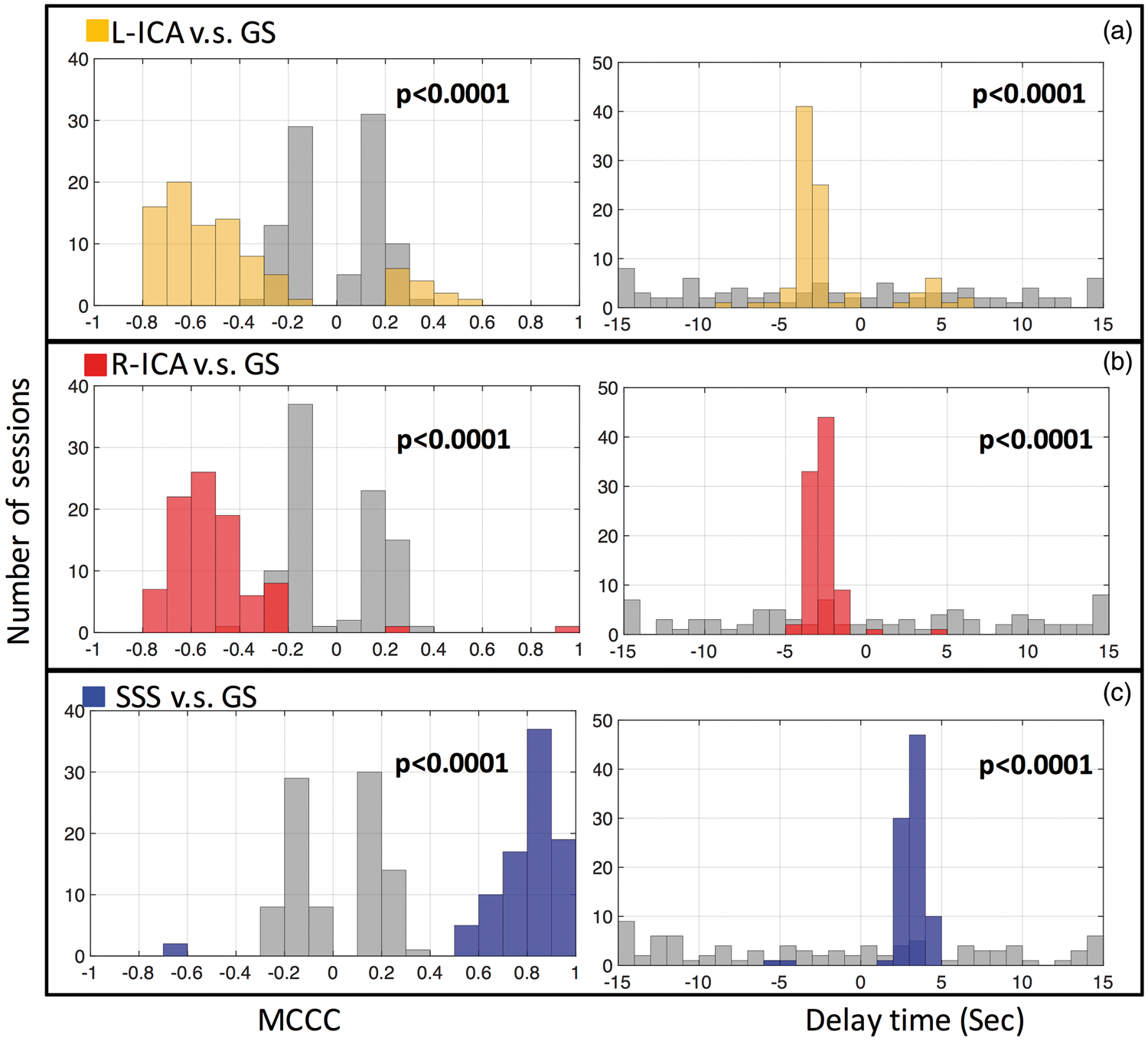

To understand the relationships between the signals in the large blood vessels (i.e. arteries and veins), we calculated the MCCCs and the corresponding time delays from 90 resting state scan sessions between right IJV and (1) SSS (blue), (2) left ICA (orange) and right ICA (red). The results are shown in Figure 6. As in Figure 4, highly consistent results with the same correlation patterns were obtained. Out of 90 resting state sessions, 84 of them have positive MCCC between SSS and right IJV (0.7 $1\pm$ 0.15); 77 of them have negative MCCC between right ICA and right IJV (−0.4 $5\pm$ 0.12) and 61 of them have negative MCCC between left ICA and right IJV (−0.5 $0\pm$ 0.14). The corresponding time delays are − $1.10\pm 0.72$ s, −7. $02\pm 0.87$ s and −7. $19\pm 1.48$ s, respectively. The negative sign in the time delays mean the signals of SSS, and ICAs lead those of the right IJV. In Figure 4, we see that the sLFO signal of the right ICA leads that of SSS by about 6.07 s (2.85 + 3.22 s), while the sLFO signals of SSS leads that of IJV by 1.10 s in Figure 6. Therefore, the accumulated time delay between the ICA signal and that of the IJV is ∼7.17 s, which agrees with the 7.02 ± 0.87 s calculated directly in Figure 6. The same error assessments (as in Figure 5) were conducted and all the distributions are significant (p < 0.001). However, compared to Figure 4, the consistency and averaged MCCC values from these sessions are lower. The main reason is that the SNR of the signal from the IJV is lower than that of the GS because of the limited number of voxels involved in calculating IJV signal and the proximity of IJV and ICA, leading to possible cross-talk.

Figure 6.

(a) Maximum cross-correlation coefficient (MCCC) calculated from 90 resting state scan sessions, between right IJV (R-IJV) and: SSS (blue), left ICA (L-ICA: orange) and right ICA (R-ICA: red). The distributions of these MCCCs (between −1 and 1) are shown in the graph on the right with matching colors. The 90 time delays corresponding to MCCCs in (a) are shown in (b) with its distribution graph on the right. The averaged MCCC and time delay were calculated for the main distribution clusters. P values are the results of a two sample Kolmogorov–Smirnov test between each MCCC/time delay and noise distribution (not shown). P value in each graph represents the common values for all three distributions.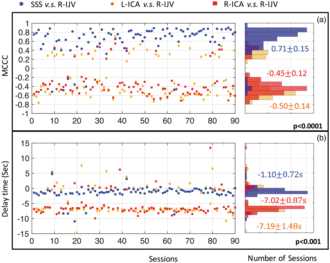

Discussion

In this study, we have demonstrated the following on the publicly available MyConnectome dataset. First, significant, but negative, correlations (˜−0.5) were found between the sLFO BOLD signals extracted from the ICAs and (1) the GS; (2) the SSS and (3) the IJVs. Second, we found the consistent time delays between these sLFO signals from ICAs, GS and veins, which coincide with the blood transit time through the cerebral vascular tree. In the discussion, we will talk about the physiological meanings of these findings and their implications. Moreover, we will discuss the possible confounds in our analytical processes.

Maximum correlations: BOLD signals in arteries with that from the GM and the veins

Figures 4(a) and 6(a) show that the low-frequency components of the left and right ICAs time courses are consistently correlated with the GS and the IJV signals, however, with a negative sign. This result supports our hypothesis that the sLFO BOLD signals can be found in the arteries, with time delays indicating that they precede the signals in the brain. The same sLFO seen in the GS is also consistently found in the SSS (MCCC = 0.81) and IJV, in accordance with the hypothesis that the sLFO travels with the blood throughout brain, drains into the SSS, then moves to the IJVs. To our knowledge, this is the first study to follow a particular physiological component of the BOLD signal (i.e. sLFO) throughout the entire cerebral vasculature, including the arteries, capillary bed and veins.

The finding of negative MCCC values (between the sLFO BOLD signals of arteries and those of GS/IJV) is interesting, particularly as no fMRI study has ever focused on large blood vessels such as the ICAs (typically excluded from scanning or removed in the preprocessing steps). We hypothesize the cause for our observation to be the high oxygen saturation in arteries (∼100%) coupled with dynamic partial-volume effects with surrounding tissue, which are modulated by cerebral blood volume (CBV) changes in ICA. In short, the BOLD signal is influenced by the volume susceptibility difference between blood and tissue ( $\Delta \chi )$ , which can be expressed as ²³

$$\Delta \chi =\mathit{HCT}*((1-Y)*(\Delta {\chi }_{\mathit{deoxy}}-\Delta {\chi }_{\mathit{oxy}})+\Delta {\chi }_{\mathit{oxy}})$$

(1)

Here $\Delta {\chi }_{\mathit{deoxy}}$ and $\Delta {\chi }_{\mathit{oxy}}$ represent the relative susceptibility of deoxygenated and oxygenated blood to tissue respectively. Y is the oxygen saturation. HCT is hematocrit. Figure 7 shows the $\Delta \chi$ as a function of Y as predicted by equation (1) (based on the work of Weisskoff and Kiihne ²³ ). We can see that $\Delta \chi$ changes sign at a Y value of ∼86%. In other words, the sign of $\Delta \chi$ is negative in large arteries (e.g. ICA) relative to the capillaries/veins, which leads to opposite signs in BOLD. Strictly speaking, fMRI signal in large arteries, such as the ICA, can be different from the common BOLD contrast, where $\Delta \chi$ would change as blood oxygenation changes due to neuronal activation. For a large artery where blood oxygenation is constant, $\Delta \chi$ does not change and vessel volume changes likely drive the contrast.

Figure 7.

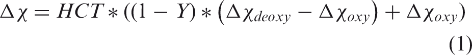
Susceptibility of blood relative to tissue as a function of blood oxygenation; 70% blood oxygenation (blue square: vein) leads to a positive value of relative susceptibility, while 100% blood oxygenation (red square: artery) leads to a negative value of relative susceptibility.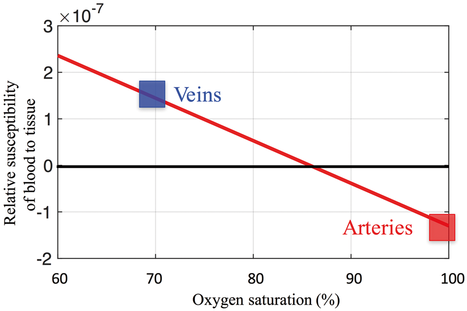

A more thorough discussion of this and other alternative explanations for the negative BOLD signal can be found in Appendix 1.

Maximum Correlations: High values between GS and SSS

It is well-known that BOLD contrast depends on the difference in susceptibility between blood and tissue. It tends to bias the sensitivity of fMRI towards venules and veins, where blood is less oxygenated, and therefore the concentration of deoxy-hemoglobin, and thus the susceptibility difference is greater. ²⁴ This is one major reason that the GS is highly correlated (MCCC = 0.81) with BOLD signals from the large veins, such as SSS. The other reason is that these sLFOs are widespread throughout the brain, as they travel with the cerebral blood flow. ¹³ In contrast, neuronal activations, such as those studied in resting state analyses, are generally more regional and cause local BOLD signal changes, which are likely smoothed/canceled out during the GS calculation, leaving the sLFOs as the dominant signals in the GS. This explains the positive correlations between the GS and the SSS/IJV sLFO BOLD signals. This study, together with others, ²² explored the vascular component of the GS. However, there are many other components of the GS, as clearly summarized in a recent publication by Liu et al. ²⁵ In addition to the nuisance components, such as motion, physiological fluctuation and vascular contribution, the GS has also been linked to LFP power fluctuations, ²⁶ vigilance status measured by EEG,^27,28 and arousal fluctuations. ²⁹ Moreover, it has been found that the variance of the GS ³⁰ and the global connectivity are associated with different brain pathologies. ³¹ Due to the limitations of the retrospective analysis performed in this study, we did not explore these other components.

Maximum correlations: Relatively low values between the GS and ICAs

The peak cross-correlation value between the ICA signal and the GS, while still quite significant, is lower than that of the SSS and GS. There are several factors that may contribute to the lower correlation.

Due to scan field of view, only a limited section of the ICA can be found in fMRI data, while the entire SSS can be used. This, in conjunction with the relatively small cross-section of the ICA’s lead to a lower signal-to-noise (SNR) for the arterial signals.

The power of the GS/SSS BOLD signals is concentrated in the low frequency range (<0.1 Hz), whereas the BOLD signal energy in ICAs is widely spread as shown in Figure 2. The frequency spectrum of the BOLD signal in the ICA includes not only the LFOs, but also high-frequency oscillations. These high-frequency oscillations are mostly from cardiac pulsation and respiration due to aliasing.

Arterial blood has time varying T1 inflow effects due to fresh blood coming into these voxels at varying speed, ³² causing complicated modulation of the signal intensity, again adding signal variance, which will lower the relative contribution of the sLFO signal.

Delay time: The meaning of delays

Figures 4 to 6 show the consistent delay values between sLFO BOLD signals from different regions. For instance, the delay between sLFO fMRI in the ICA with the GS is about 2.85–3.04 s (signal from ICA is leading). The delay between the GS and the sLFO in the SSS is about 3.22 s (the GS leads). The delay values are highly consistent (Figures 4 to 6), which indicates that the underlying physiological phenomenon is robust. More importantly, the order of arrival time derived from the different delay values matches the known structure of the cerebral vasculature: the ICA signal leads the GS by ∼3 s, which leads the SSS by a similar amount, which in turn leads the IJV by ∼1.1 s. The delay values measured directly from ICA to IJV (7.02/7.19 s in Figure 6) are consistent with previous measures of cerebral circulation time, which found delays of 7.5 ± 1.8 s from the carotids to the jugulars using echo contrast-enhanced ultrasound in 64 healthy subjects. ²⁰ This offers the strongest support of our hypothesis. However, other studies (mostly with ultrasound) have found smaller values (4.9–6.4 s)^33,34 in cerebral circulation times. This may be due to methodological effects such as the location of the measurements or definition of arrival time in the observation curve, etc. In section “Effects of bandpass filtering” in discussion, we also discuss the effects of bandpass filter range on the delay time calculations. In summary, our study offers a novel and simple way to assess cerebral circulation time by fMRI directly without using exogenous contrast agents, and one that is consistent with the literature. However, the accuracy will have to be evaluated by careful studies.

Lastly, we calculated the MCCCs and time delays between the signals of two ICAs and two IJVs. The positive MCCCs (0.46 ± 0.14 and 0.59 ± 0.16) were obtained between the two ICAs and two IJVs, respectively, with almost zero time delays (−0.20 ± 0.84 s and −0.94 ± 1.23 s). Judging by the structural and functional similarities of these two pairs of vessels and their matching distance from the heart/lung system, it is natural to expect that the similar BOLD signals should be observed at these two ICAs/IJVs at same time. The consistent high MCCCs and close-to-zero delays offer further validations of the methods and the hypothesis. Moreover, it indicates the accuracy in the registration procedures, i.e. ICAs and IJVs are accurately identified in the fMRI data, in this study. The details information can be found in Figure A.1. of SM.

Delay time: What is the sLFO (volume effect)

We have demonstrated in this study that the sLFO BOLD signal appears in the arteries prior to any location in the brain (albeit inverted). From there, it passes through arterioles, capillaries, venules and finally drains out through the veins. The origin and function of this sLFO are still not clear.^35,36 These physiological oscillations overlap with resting state oscillations in frequency (<0.1 Hz) and both contribute to the BOLD signals. Since it is hard to isolate the resting state portion of the BOLD signal in humans, it is almost impossible to compare these two signals directly in an fMRI dataset. However, from previous correlation studies, we have found that sLFOs can explain up to 50% of the variance of the BOLD signal in the LFO band. ¹⁰ Animal studies may help to resolve this question, ³⁷ as both neuronal firing and vascular fluctuations can be recorded by different modalities at same time, ³⁸ and small animals seem to have physiological oscillations at somewhat higher frequencies. ³⁹ Many researchers have tried to link these sLFOs with respiration depth and cardiac rate changes.^6,7,40 However, a recent study ²¹ found that these LFOs derived “directly” from the respiration and heart rate are likely not the sLFO we have observed in the brain and periphery. Mayer waves are well-known oscillations of about 0.1 Hz in humans. ⁴¹ They are believed to be arterial blood pressure changes closely correlated with sympathetic nerve activity. Thus, it is a global synchronous wave, which is unlikely the source of sLFOs (which travels). Vasomotion, on the other hand, is spontaneous oscillation in the vascular tone, which is independent of respiration, pulsation and neuronal activity.^42–44 In an intriguing human study, Rayshubskiy et al. ⁴⁵ found the 0.1 Hz oscillation in awake human cortex which travels to different regions of cortex using intraoperative multispectral optical imaging. Based on this, they concluded that the travelling wave was likely to be vasomotion, which matched the observations in this study. Similarly, Bumstead et al. ³⁹ observed waves of oxy-hemoglobin concentration travelling across the mouse cortex using optical intrinsic signal imaging. In addition, it has long been known that at least a portion of the low-frequency physiological signal reflects the slow fluctuations of CO2 (a potent vasodilator) in the blood,^46,47 which will dilate vessels locally as it travels with the blood. This, together with vasomotion, is consistent with the idea that the negatively correlated arterial signal comes from changes in the blood volume of the bright arterial blood, which will be opposite in sign to volumetric changes in dark, venous blood. In summary, the sLFO appears in the arteries before entering the brain, is possibly a blood volume effect and travels with the blood throughout the brain from large arteries to large veins.

Possible confounds: Effects from cross correlation

As we know, low pass filtering and picking the peak cross correlation in a window inflate the correlation coefficient, and lead to the possibility that correlations are spurious.^21,48 Based on a previous study, ²¹ we concluded that a correlation value of MCCC > 0.28 (or MCCC<−0.28) is required to achieve P < 0.01, when both filtering and cross correlation are used in the process. Most MCCC values calculated in this study are larger than 0.28 (or <−0.28). For a more robust test, we conducted the so-called “mismatch” correlation calculation, in which the distribution of random correlations was estimated by filtering and cross correlating the similar, however, “mismatched” data. Then we used two sample Kolmogorov–Smirnov test to measure the significance of our “matched/real” findings, compared to the corresponding noise baseline. The result of this “mismatch” correlation calculation is shown in Figure 5. From the figure (black distribution), we can see that the MCCCs are clustered around ± 0.2 and time delays are widely spread between −15 s and 15 s (correlation window), which are consistent with the previous studies on the spurious correlations. Our results in Figure 4 and 6 are significantly different from these spurious distributions with p < 0.001. This confirms that our results are not from spurious correlations. However, there is another type of error, caused by a “periodicity effect.” For example, in Figure 4(b), most of the positive time delays (left ICA and GS) are clustered around +5 s, while in Figure 6(b), many delays (left ICA and right IJV) are clustered around 0 s. This effect arises because the random sLFO fluctuations are occasionally pseudo-periodic, i.e. there is one dominant low-frequency component. The MCCC calculated involving this periodic signal can be either positive or negative (influenced by factors such as noise) with time delays differing by the half of the period if we select the “wrong” correlation peak. This explains two things: (1) since the periodic signal is real signal, not noise, the magnitude of the MCCC is likely larger than 0.2; (2) the corresponding delays are likely clustered around a value which is about half period away from the true value.

Possible confounds: Motion artifacts

The Myconnectome project did not record the physiological signals, such as pulse and respiration, so we cannot directly assess physiological effects. However, since the TR is 1.16 s, the respiration, which is normally around 0.2 Hz, will be fully sampled by the resting state scan. ⁴⁹ This is confirmed by examining the motion parameters. When studying motion parameter (details in Figure A.2. of SM), we found that the respiration-related motion (∼0.15 Hz) is a dominant, highly periodic signal and can be seen in both rotational and translational parameters. However, the LFO (<0.1 Hz) is not prominent in the motion parameters (except the very low frequency drifting < 0.005 Hz). Further study of the relationship of motion and the GS showed the following points. First, there are significant correlations between the GS and motion parameters with both positive and negative MCCCs, even if the GS is calculated after motion correction. These observations are consistent with recent work from Power et al. ⁵⁰ Interestingly, if we assume that motion affects voxels simultaneously, then there should be no clear time delays between motion parameter and the GS, and this is what was observed. Furthermore, we found that, unlike the GS, the motion does not affect the ICA BOLD signal in the frequency band of 0.005–0.1 Hz. The motion-related information is shown in Supplemental Figure A.2 to A.4. Lastly, we extracted the BOLD signals from white matter (WM), gray matter (GM) and the lateral ventricles (LVen) (Supplemental Figure A.5), as WM and LVen signals are more prone to respiration and cardiac influences.^51,52 The results indicated that sLFOs are present in the BOLD signals of the WM and GM, but not in the ventricles. The consistent time delay from GM to WM matched our previous dynamic susceptibility contrast study, where blood was shown to be arrive in WM after GM. ¹⁴ These findings are consistent with sLFOs being blood-borne signals, which present widely in the brain with delays matching the flow paths.

Possible confounds: Effects of bandpass filtering

To assess the effect of bandpass filter selection on MCCCs and time delays, we performed the same analyses with two additional bandpass filter ranges, 0.1–0.2 Hz and 0.005–0.2 Hz. The results (Supplemental Figures A.6 and A.7.) are largely consistent. However, due to the periodicity effect (i.e. dominant respiration signal) discussed previously, both positive and negative MCCCs were found in Figure A.6(a) together with many “peaks” observed in Figure A.6(b). Nevertheless, for most sessions, the ICAs’ signals lead the GS by about 2 s, while the SSS signals lag it by about 2 s. These values decreased from those in Figure 4, which may indicate that the blood vessels/blood are a dispersive medium for these waves. As they propagate through the brain, low-frequency oscillations may travel slower than the higher frequency (i.e. likely respiration-related) oscillations. The shortened cerebral circulation time matches the results of some studies. As we know, respiration directly affects the BOLD signal through motion and susceptibility changes. ⁵³ It should make synchronized BOLD changes throughout the brain. However, the spatially varying delays we observed in the 0.1–0.2 Hz frequency range show that the effect of respiration is likely indirect, from resulting CO2 fluctuations in the blood, instead of motion/susceptibility.

We also examined the range of 0.005–0.2 Hz (shown in Figure A.7. of SM), which combines the range of 0.005–0.1 Hz and 0.1–0.2 Hz. Again, the result of MCCCs and time delays are very consistent and significant. The ICAs’ signals lead the GS about 2.3 s, while SSS signals lag the GS about 2.58 s. This result is between those from the fast traveling wave (0.1–0.2 Hz) and slow traveling wave (0.005–0.1 Hz; Figure 4), and could be considered as the “averaged” propagation rate. In summary, the MCCCs and arrival time order calculated between BOLD signals of different blood vessels and GS are robust, regardless of selection of filtering range. Moreover, our findings suggest the vessel/blood might be dispersive. Further study is warranted into the nature of different oscillations and their relationships with the blood flow.

Limitations and future work

There are several limitations in this study, which we hope to address in the future work.

First, we do not conclusively understand the negative correlations between the BOLD signals from big arteries and big veins. Existing models of the BOLD signal have generally focused on vessels much smaller than a voxel, rather on vessels of comparable or larger size. We will seek to clarify this by doing high-resolution fMRI imaging or dynamic vessel wall imaging in the future. Second, no physiological waveforms, such as respiration and cardiac pulsation, were recorded in the study. Having these recordings would help elucidate their effects in the large blood vessels and the GS, and their contributions to the sLFO. In a future study, we will include these physiological measurements. Finally, as this study was performed on the data from a single individual, it is possible that this finding is unique to this subject. However, this is unlikely because all the metrics related with the venous and capillary sLFO signals were extremely consistent with our previous work^13–15 on groups of subjects. Future confirmation in a more heterogeneous subject pool will be the logical next step.