Sage Journals: Discover world-class research

Abstract

We analyze the pulsatile signal component of dynamic echo planar imaging data from the brain by modeling the dependence between local temporal and spatial signal variability. The resulting magnetic resonance advection imaging maps depict the location of major arteries. Color direction maps allow for visualization of the direction of blood vessels. The potential significance of magnetic resonance advection imaging maps is demonstrated on a functional magnetic resonance imaging data set of 19 healthy subjects. A comparison with the here introduced pulse coherence maps, in which the echo planar imaging signal is correlated with a cardiac pulse signal, shows that the magnetic resonance advection imaging approach results in a better spatial definition without the need for a pulse reference. In addition, it is shown that magnetic resonance advection imaging velocities can be estimates of pulse wave velocities if certain requirements are met, which are specified. Although for this application magnetic resonance advection imaging velocities are not quantitative estimates of pulse wave velocities, they clearly depict local pulsatile dynamics. Magnetic resonance advection imaging can be applied to existing dynamic echo planar imaging data sets with sufficient spatiotemporal resolution. It is discussed whether magnetic resonance advection imaging might have the potential to evolve into a biomarker for the health of the cerebrovascular system.

Keywords

Brain imaging magnetic resonance imaging cerebral hemodynamics magnetic resonance angiography mathematical modeling

Introduction

Propagating waves can reveal information about the medium they are traveling in. Wave characteristics, such as waveform, wavelength, velocity, and dispersion, often depend on the physical parameters of the medium. Cardiovascular pulse waves in the human body provide a natural physical disturbance to the vascular system whose effects have been utilized in clinical diagnostics for a long time. For example, pulse wave velocity (PWV) measurements in major arteries reveal information about arterial compliance.¹ Arterial compliance, the ratio of blood volume change to blood pressure change, is an important physiological factor by absorbing the impact of the cardiac pulse pressure waves and enabling steady blood flow throughout the whole cardiac cycle.^2,3 The PWV is a reliable prognostic marker for cardiovascular morbidity and mortality in adult populations such as the elderly, patients with diabetes, and hypertension.⁴ More important for the brain are the findings that aortic stiffness is associated with cerebral small-vessel disease in hypertensive patients,⁵ that cognitive decline correlates with PWV,⁶ and that neurodegenerative diseases such as Alzheimer’s disease are thought to be related to cerebrovascular dysregulation.⁷ Furthermore, the understanding of emerging concepts such as pulse wave encephalopathy would be aided by novel diagnostic imaging methods of cerebral vasculature.^8–12 However, there are only limited in vivo options for imaging vascular dynamics in the human brain. Arterial spin labeling (ASL) is probably the most advanced current method with the highest spatial resolution.^13,14 It provides quantitative blood flow values in the capillary bed, assuming steady flow.¹⁵ In contrast, the important parameter of arterial compliance depends on the pulsatile component of the flow. It can be imaged for larger vessels locally with transcranial Doppler ultrasound¹⁶ but also, over the whole brain, with specific ASL pulse sequences.^17,18 Pulsatile flow components can also be imaged over the whole brain with 4D phase contrast angiography.¹⁹ Nevertheless, it would be highly desirable to have more imaging modalities at hand to investigate the pulsatile component of cerebrovascular dynamics.

In this article, we present phenomenological findings resulting from a spatiotemporal analysis of dynamic magnetic resonance imaging (MRI) data, as it is routinely acquired in functional imaging of the brain. Linear modeling of the dependence between local spatial and temporal signal variability results in a wave equation for unidirectional waves, a form of advection equation. The resulting imaging technique, which we term magnetic resonance advection imaging, or MRAI, provides velocity vector maps related to pulsatile dynamics obtained from dynamic MRI data. We aim at showing that MRAI has the potential to provide precisely localized information about pulsatile dynamics. This information might aid the interpretation of functional MRI and resting state brain network connectivity mapping, which is affected by vascular anatomy;^20,21 for example, MRAI maps allow for the identification of local pulsatile components derived directly from echo planar imaging (EPI) data, without the need for co-registration. These components can induce long-range signal correlations reflecting vascular (in contrast to neuronal) connectivity. Although MRAI velocity maps are not yet quantitative maps of PWV, the results presented here might facilitate development of imaging biomarkers based on PWV in future.

In the Materials and methods section, MRAI and its application to functional EPI data are described. Also, models for spatial and temporal estimation errors are proposed. Finally, pulse coherence maps (PCMs) are introduced in order to demonstrate the pulsatile nature of MRAI maps. In the Results section, we provide evidence that MRAI maps pulsatile flow.²² It is shown that inter-subject variability can be explained to a large degree, and potentially reduced in further applications, by the temporal estimation error model. The model is validated by numerical simulations. The phenomenological findings are discussed in the Discussion section with the help of further simulations, and possible future strategies to overcome present limitations are mentioned.

Materials and methods

MRAI model

Our goal is to estimate velocities of traveling waves in blood vessels from dynamic MRI data. The frequency-dependence of velocity, or dispersion, will be neglected, as will reflected pulses. In order to be able to generate spatial maps of velocity estimates, we define our model locally^23–25 in a small spatial domain Ω in which the physical vessel and blood properties, and thus the pulse shape, do not change. In practice, this could mean that in a three-dimensional data set the model is defined for example for cubes of 3 × 3 × 3 voxels. The spatial velocity estimation maps, or MRAI maps, then consist of the combination over all those domains, defining the whole imaging volume. It is assumed that the dynamic MRI signal, $ρ (r, t)$ , can be described by a traveling wave within each domain. The physiology causing the observations $ρ (r, t)$ will be discussed below. As it travels down the vessel, from one time point to the next, the wave is a spatially shifted copy of itself, as long as it stays within Ω. In other words,

ρ (r, t) = ρ (r - u t, 0),

(1) with a constant velocity u. Then, throughout Ω, ρ(r,t) obeys the advection equation²⁶

\frac{\partial ρ (r, t)}{\partial t} + u \cdot grad ρ (r, t) = 0 .

(2)

This equation simply linearly relates the temporal signal change to the spatial signal change, with the linearity coefficient u. The key idea for estimating u from the signal ρ(r, t) is that arbitrary differentiable functions of the form equation (1) are solutions of equation (2), such that the coefficients u can be locally estimated in each domain by a fit of this equation to data independent of the particular shape of ρ( r , t).

To understand the meaning of equation (2) we start with the one-dimensional advection equation, i.e.,

\frac{\partial ρ (x, t)}{\partial t} + u \frac{\partial ρ (x, t)}{\partial x} = 0 .

(3)

Equation (3) follows from the one-dimensional wave equation

\frac{\partial 2 ρ (x, t)}{\partial t 2} - u 2 \frac{\partial 2 ρ (x, t)}{\partial x 2} = 0

(4) by a factorization into right- and left-traveling waves, i.e.,

(\frac{\partial}{\partial t} + u \frac{\partial}{\partial x}) (\frac{\partial}{\partial t} - u \frac{\partial}{\partial x}) ρ (x, t) = 0 .

(5)

This equation is fulfilled if either of the two factors vanishes. The first factor, a traveling wave in the positive x-direction for u > 0, yields equation (3), demonstrated in Figure 1(a). In three dimensions, equation (2) includes situations in which the wave velocity direction is not aligned with the spatial derivative of the signal; the dot product $u \cdot grad ρ (r, t)$ indicates that only the projection of the wave velocity on the spatial signal gradient matters. Equation (2) allows for an estimation of wave velocity coefficients independent of vessel orientation with respect to the coordinate system.

Figure 1.

Traveling wave sampling scheme and multiple regression. (a) Schematics of a one-dimensional wave traveling along the positive x-direction with u > 0 and its spatiotemporal sampling by dynamic imaging. The sample points used for estimating the partial derivatives in the one-dimensional wave equation (3) shown at the top are labelled as ρ(x, t-Δt), etc. All these points lie in the same domain Ω. (This scheme emphasizes the waveform, which in real data is less pronounced.)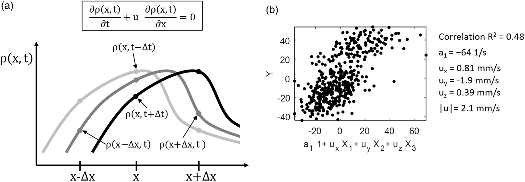

The local velocity u = (u_x, u_y, u_z) can be estimated from spatiotemporal data by multiple regression.^27,28 In order to generate maps of velocity estimates û = (û_x, û_y, û_z), we need to estimate the velocity coefficient locally for each voxel. By expanding the dot product in equation (2), the regression is linear and the regression equation reads, for example

Y = a_{1} 1 + u_{x} X_{1} + u_{y} X_{2} + u_{z} X_{3} + η + ɛ

(6) with

Y = \overset{\land}{\frac{\partial ρ (r, t)}{\partial t}}, X_{1} = - \overset{\land}{\frac{\partial ρ (r, t)}{\partial x}}, X_{2} = - \overset{\land}{\frac{\partial ρ (r, t)}{\partial y}}, X_{3} = - \overset{\land}{\frac{\partial ρ (r, t)}{\partial z}} .

(7)

The terms Y and X₁ to X₃ are estimated from data by finite differencing as described below. The hat symbols indicate estimates rather than exact quantities. The constant term ‘1’ accounts for possible time-independent offsets in the data, for example gradients defined by brain anatomy. Additional nuisance variables are denoted by the symbol η.²⁹ The unexplained variability ɛ = ɛ(r, t) is assumed to be Gaussian and independently distributed. It describes errors arising from the time derivative estimation and other influences that are not modeled by the advection equation such as motion and respiration effects. The errors of the regressors X₁ to X₃ are not included in order to avoid using a total least squares approach,^30,31 which is more prone to be ill-conditioned.³² Derivatives are estimated here with the central two-point difference scheme^26,33 as

\overset{\land}{\frac{\partial ρ (r, t)}{\partial x}} = \overset{\land}{\frac{\partial ρ (x, y, z, t)}{\partial x}} = \frac{ρ (x + Δ x, y, z, t) - ρ (x - Δ x, y, z, t)}{2 Δ x} \overset{\land}{\frac{\partial ρ (r, t)}{\partial t}} = \frac{ρ (r, t + Δ t) - ρ (r, t - Δ t)}{2 Δ t} .

(8)

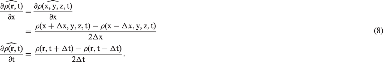
The y and z derivatives are computed equivalently to the x derivative. This scheme has the advantage over more accurate higher order schemes that only nearest neighbor points of r have to be taken into account.

Figure 1(b) shows an example for the regression applied to the data point marked with a red dot in Figure 2(c). Once model (2) has been fitted to each voxel time series of the dynamic MRI data via equation (6), MRAI maps can be obtained, showing either the magnitude (Figure 2(c)) or the direction of û (Figure 2(d)).

Figure 2.

Magnetic Resonance Advection Imaging (MRAI). (a) Maximum intensity projection (MIP) of a time-of-flight MR angiography image of a healthy human brain at 7.0 T (Subject 16). (b) MIP of a PCM of the same subject, computed from a functional EPI scan. Bright pixels indicate a high maximum coherence between pulse oximetry time series and EPI signal. (c) MIP of an MRAI map. Bright pixels indicate high advection velocity coefficient estimates and the red dot marks a voxel that is used to demonstrate the regression approach in Figure 1(b). (d) Color-coded direction map displaying the directions of the estimated MRAI velocity vectors. Directions are indicated in the inset as green – anterior/posterior, red – right/left, blue – superior/inferior direction.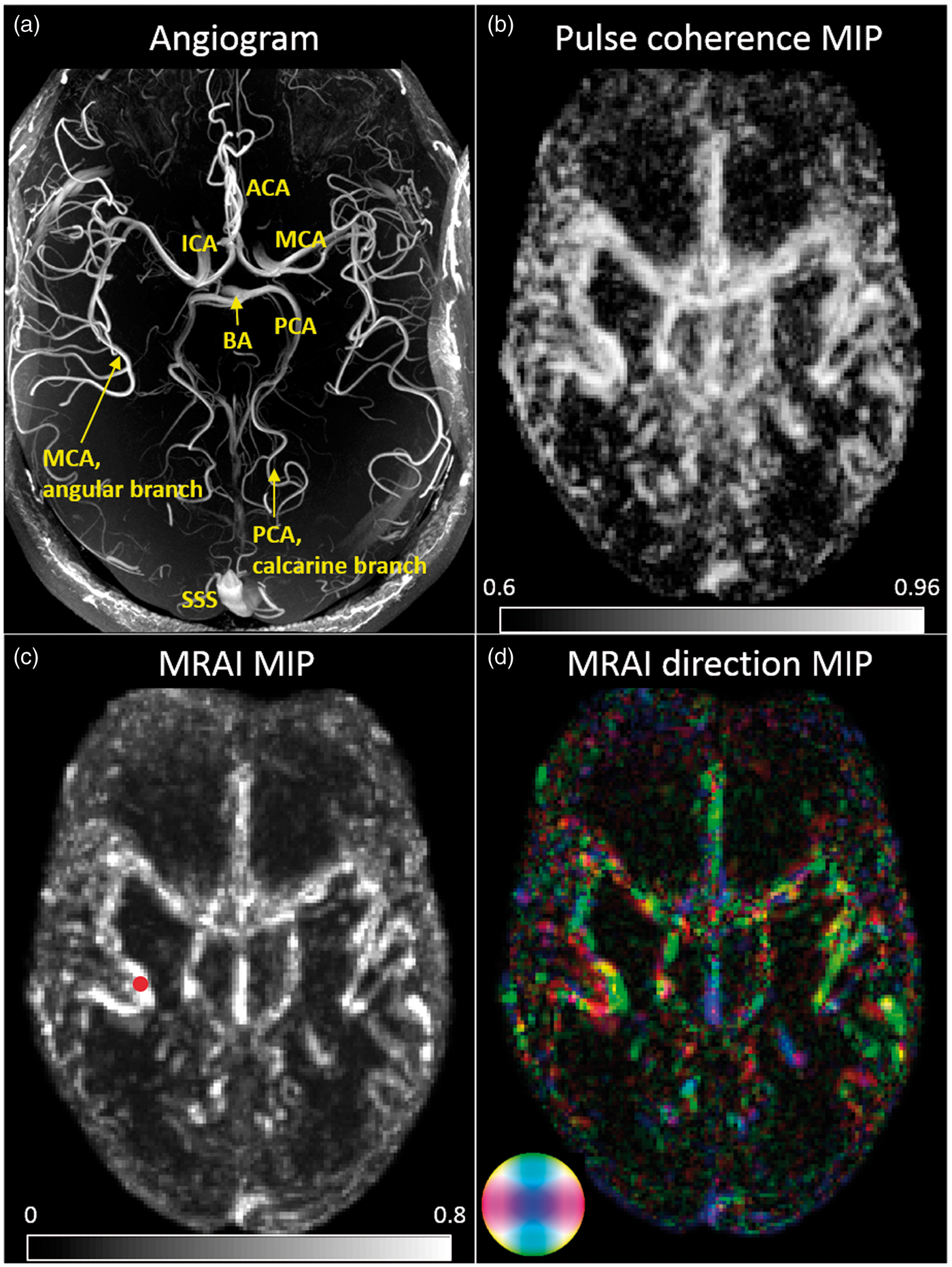

MRAI physiology

We assume that traveling waves described by the MRAI model above are related to blood volume waves. For example, for a blood vessel along the x-direction, equation (3) can describe the x-component of the pulsatile component of the blood flow velocity, and u is then defined as the PWV. The same advection equation also holds for blood pressure waves,³⁴ which, via the Windkessel model,³⁵ are a function of the integrated net flow into the vessel reservoir.³⁶ Since the local blood volume is related to local blood pressure via the compliance C as dV = C dp, the same advection equation applies to the pulsatile component of the blood volume (or vessel expansion) as well. The value of the velocity u is always the same, no matter whether the signal $ρ (x, t)$ reflects the pulsatile component of flow velocity, pulse pressure, or pulsatile component of blood volume. In general, for voxels that are affected by the expansion of blood vessels, for example via blood pressure, neurovascular coupling,^37–39 or other mechanisms,⁴⁰ it is reasonable to assume that the MRI signal $ρ (r, t)$ reflects this volume change.

If $ρ (r, t)$ reflects pulsatile volume changes, u can be interpreted as the PWV. The PWV in arteries, or Moens-Korteweg velocity,⁴¹ carries information about their physiology, via the Moens-Korteweg formula^42,43

u = \sqrt{\frac{Eh}{ρ_{B} d}} .

(9)

As per this model, three vascular parameters determine the PWV: Vascular diameter d, wall thickness h, and the vessel’s elastic (Young’s) modulus or distensibility, E. The density of the blood, ρ_B, can be approximated as constant for our purposes. To be a valid description of PWVs, it is assumed that vessels are considered to be elastic tubes with isotropic walls,⁴⁴ which experience isovolumetric change with pulse pressure. Notably, pressure gradients, which would be required to determine blood flow, are absent in the Moens-Korteweg formula. Therefore, PWVs can be modeled independently from blood flow, and in fact, can be one to two orders of magnitude faster than the latter.⁴¹ Constant flow contributions to the signal cannot be extracted by parameter fitting to the advection equation (2) anyhow, as they do not cause any temporal signal change. Signal variability, however, could occur if the blood has inhomogeneous properties in the model domain Ω, which may be caused by variations in oxygenation or temperature or any other property that might affect the particular MRI contrast, for a given MR pulse sequence. Here, we assume that those contributions are negligible in comparison to pulsations.

Aliasing

A cerebral pulse wave with a velocity of 10 m/s has a wavelength of 10 m if the pulse frequency is 1 Hz. This is in stark contrast to typical EPI sampling rates, including the spatial sampling of 1.2 mm and the temporal sampling rate of 2 s of the data set analyzed for this work.

In the following, it is detailed how sampling affects the estimation of wave velocities via aliasing, and a correction factor is provided under the assumption that the pulse signals are periodic. In the Results section, it is shown that by using this correction factor the data can be unbiased to a certain degree, reducing inter-subject variability. The derivation of the correction, or bias factor, is given in Supplementary Information S1 and can be summarized as follows: the velocity is estimated from data by finite differencing applied to the wave equation (3). The resulting analytic relation shows that the estimated velocity is proportional to the true velocity, with a factor that depends on the heart rate. This factor, if different from zero, can then be used to correct the velocity estimate. The bias correction follows under the assumption of a sinusoidal wave

ρ (x, t) = ρ_{0} sin (α (x - ut)) with α = \frac{2 π}{uT}

(10) as

û = sinc (\frac{2 π Δ t}{T}) u .

(11)

Equation (11) holds for our sinusoidal model with fixed T, but in practice the waveforms are more complex and T varies with the heartbeat, so the bias factor is an approximation.

Wavelength limits

The wavelength of a traveling pulse wave is much longer than a typical MRI spatial sampling interval and limits the maximum possible velocity estimates under given signal-to-noise ratio (SNR). In order not to compromise quantitative estimates of wave velocities in an unacceptable way, either spatial derivatives have to be estimated by other means than finite differencing, or the SNR has to increase considerably, or both. In Supplementary Information S2 an approximation for the maximum possible wave velocity is derived. It is validated in Figure 3(c) on numerical simulations.

Figure 3.

Understanding estimation bias. (a) Regression between the average MRAI velocity coefficient estimates over the whole imaging volume for all 19 subjects against their average heart beat interval during the MRI scan. The two subjects with the lowest MRAI estimates, Subjects 1 and 2, as well as subject 16 from Figure 1, are labelled for comparison with the MRAI maps in Figure S1 and S2 and Figure 2, respectively. The regression is not significant (p > 0.05). (b) Regression between average MRAI velocity coefficient estimates and the magnitude of the aliasing factor (11) derived from a sinusoidal model of traveling pulse waves. The aliasing factor depends on the pulse period relative to the sampling rate of the data. It explains about half of the inter-subject variability and the regression is significant with p < 0.0005. The same subjects as in A are labelled here again. One can see that for example Subject 2, which had no useful MRAI image, has an aliasing factor of approximately zero, such that MRAI is not applicable to Subject 2 with the given sampling rate. (c) Estimated wave velocities from noisy simulations via Eq. (10). Shown are in dependence of given wave velocity u the expected estimated absolute velocity (black line), the estimates for an SNR = 32 (black asterisks), for an SNR = 64 (red asterisks), and for an SNR of 96 (green asterisks). In addition, the vertical dashed lines mark the respective expected maximum meaningful velocity. (Parameters: The SNR of 32 was determined from the data at the red dot of Figure 2(c) as the ratio of signal and background noise standard deviations. The expected wave velocities were corrected by a bias factor of -0.055 following from an average heart beat interval of T = 0.72 s from the same data set and the experimentally given temporal and spatial sampling rates of 2 s and 1.2 mm, respectively.)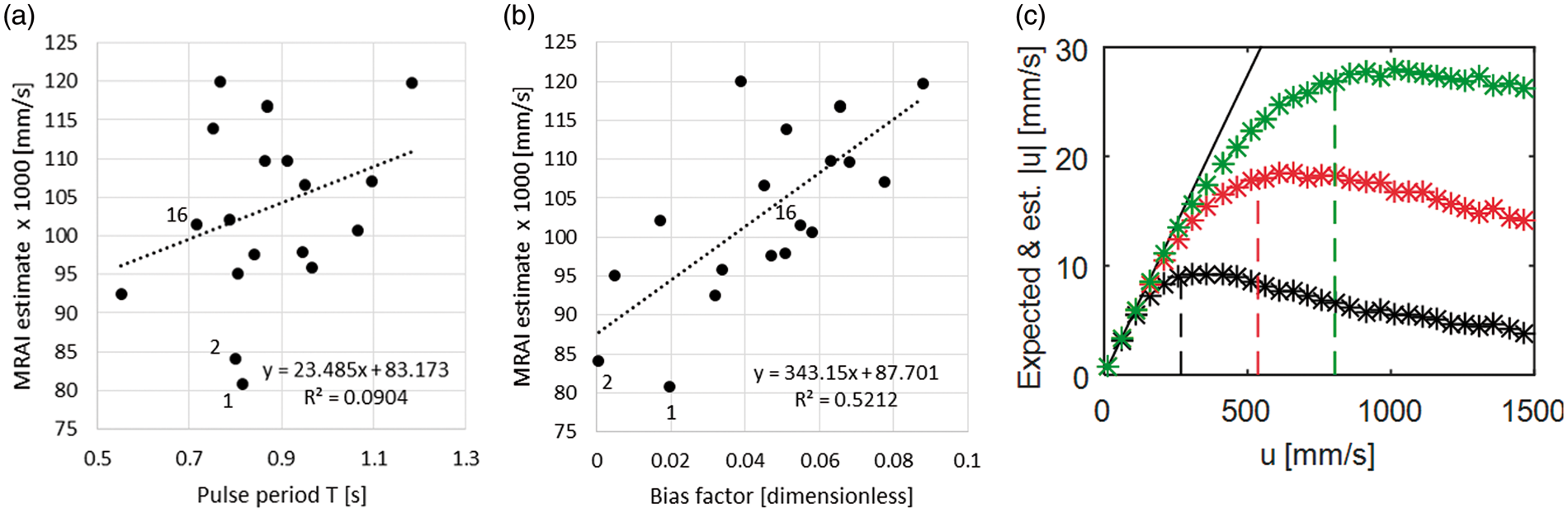

Pulse Coherence Maps

Another concept defined at this place are pulse coherence maps (PCMs). They show the coherence between a pulse-related time series, for example obtained by a plethysmograph (pulse oximeter) from a finger, and each voxel time series of the dynamic MRI signal (Figure 2(b)). Even though the pulse frequency typically is higher than typical EPI sampling frequencies, PCMs clearly depict meaningful vascular signal components. Since the magnitude of the coherence is invariant under signal time shifts, PCMs do not require re-ordering or time-shifting the MRI data in order to take account for the unknown time delay between the pulse measured at the finger and in the brain.²² The PCM is defined as

PCM (r) = max [coherence (pulse (t), ρ (r, t))] .

(12)

Here, coherence(.,.) denotes the normalized magnitude of the cross power spectrum density over its two arguments. It is a function of frequency, and the maximum is taken over a suitable frequency range. The frequency itself at which the maximum is attained is of no further interest as it normally approximates the average pulse frequency. The signal pulse(t) can be obtained from pulse oximetry data by resampling to the sampling time points of the dynamic MRI data. The signal $ρ (r, t)$ is the raw dynamic MRI signal.

Natural stimulation functional magnetic resonance imaging data set

PCMs, MRAI velocity and direction maps were computed for all 19 subjects of a publicly available natural stimulation dynamic EPI data set obtained on a 7.0 T MRI scanner.⁴⁵ During scanning, subjects were listening to an audio version of a movie. This data set includes eight 15 min long segments for each subject of which the second one was used for analysis. The transversal slices covered most of frontal and occipital cortex and the regions in between. Data were sampled with a pulse repetition time (TR) of 2 s and an isotropic spatial resolution of 1.4 mm. The data set also contains time-of-flight angiography images of about the same coverage as the EPI data (Figure 2(a)), as well as pulse oximetry data.

For this study, all analysis was performed on MNI152-transformed,⁴⁶ geometric distortion, and motion corrected EPI data sets, with an isotropic spatial resolution of 1.2 mm. In order to test for possible effects of the transformation to MNI space, the analysis described below was also compared with selected raw data sets, with comparable results (not shown).

PCMs were computed from equation (12) with Matlab 2012b (The MathWorks, Inc., Natick, MA, USA), using the function cpsd, over all voxels inside the brain using masks. The maximum in equation (12) was computed over all but the lowest frequencies (cutoff = 0.0136 Hz), in order to exclude trend effects. The signal pulse(t) was obtained from the pulse oximetry data by spline interpolation (Matlab function interp1). The resulting maximum coherences were saved to a file for each of the subjects. PCMs (Figure 2(b)) were generated from these files by a maximum intensity projection (MIP) along the z-axis (head to foot) over slightly spatially smoothed maximum coherence values. For display, values inside the range [0.6, 1.0] were used in order to only show significant contributions.

MRAI velocity maps were computed with Matlab via equation (6): First, the data were high-pass filtered with a cutoff at 0.05 Hz (Matlab function idealfilter) in order to remove components caused by low-frequency signal components.^47,48 Next, finite differences were computed following equation (8). The six motion parameter time series were used as additional nuisance regressors η in equation (6). Equation (6) was solved using a least-squares estimator (Matlab symbol “\”). The velocity estimate û = (û_x, û_y, û_z) was saved component-wise to three files for each subject. MRAI velocity maps (Figure 2(c)) were generated from these files by a MIP over slightly spatially smoothed velocity magnitudes û = ||û|| (Euclidean norm). To optimize image contrast, values above 0.8 mm/s were capped at 0.8 mm/s, corresponding to bias-corrected velocity of 15 mm/s for the subject of Figure 2. The maximum observed value was 6.3 cm/s (bias corrected).

MRAI direction maps were generated from the velocity component files by first assigning RGB values to the three velocity components: Red for û_x (brain right/left), green for û_y (brain anterior/posterior), and blue for û_z (brain superior/inferior) direction. Next, a MIP was generated by using only those voxels that found entry into the MRAI velocity MIPs as defined above. Finally, all RGB values were divided by the maximum RGB value in the MIP and the resulting map divided by a factor of 0.6 inorder to enhance colors.

Numerical simulations

In order to show performance and limitations of the MRAI fitting procedure with respect to both magnitude and direction of velocity vectors, numerical simulations of a traveling wave in a planar half-ring structure were performed. Although the MRAI model assumes physical homogeneity within the local domain Ω, this assumption is not always realized in experimental data and was taken into account with a spatial modulation profile across the ring structure, as described in the following.

Traveling waves were generated in Matlab for varying velocities as given in the leftmost column of Figure 4. Guided by possible multiband EPI acquisition parameters, the spatial resolution was set to Δx = Δy = 1 mm, the temporal resolution was Δt = 0.2 s, and 100 (space x) × 50 (space y) × 500 (time) data points were simulated. The center radius of the half-ring was r₀ = 38 mm and the width was 19 mm. Traveling wave simulations were performed only in the region defined by this half-ring. Traveling waves were defined as traveling along the ring depending on the radius r²= x²+ y² in the following way: Local velocity coefficients u = (u_x, u_y) were constant along the line r = r₀ and adjusted for other radii such as to cause wavefronts that were always parallel to the ring radius at their position (see Figure 4, data snapshot for u = 1 cm/s). The resulting velocity magnitudes u = ||u|| are shown as gray scale values in the panel labelled “Modelled velocities”. The phase angle was defined as ϕ = atan (y/x) and the path length as L = r ϕ. Then the traveling wave signal was modeled as

ρ (x, y) = m (x, y) sin (2 π / T (L / u - t)) + ɛ (x, y) .

(13)

Figure 4.

Numerical simulations. Top row: Description of the simulated traveling wave on a curved path. The middle column shows the pulse wave velocities as gray values and the wave direction. The right column shows the color code for the velocity direction. The left column shows an amplitude profile reflecting narrow outer half-rings with increased/decreased signal amplitudes.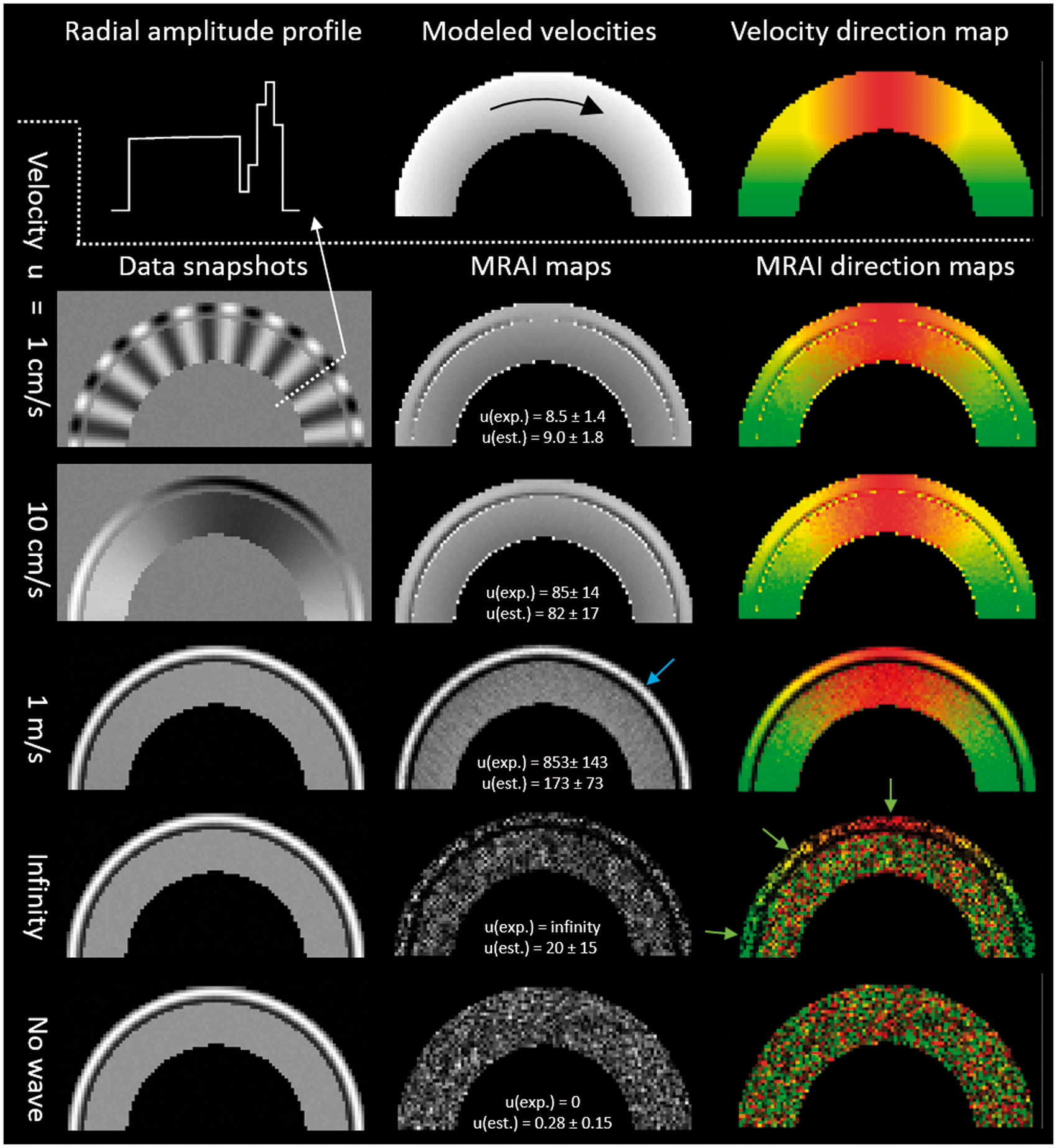

The modulation function m(x,y) consisted of a sinosoidal function of the radius only and was used to model the outer ring of increased/suppressed amplitudes. This modulation is visible in Figure 4, panel “Radial amplitude profile” and in the data snapshots. The period of the wave was T = 1.234 s and the noise ɛ(x,y) was normally distributed with mean zero and standard deviation of 0.01. With these parameters, the maximum velocity that could still be quantitatively estimated, would be about 25 cm/s. Modeled velocities were u = 1 cm/s, 10 cm/s, 1 m/s, and infinity, which corresponds to a standing wave (Figure 4, second row from bottom). In additon, MRAI maps were fitted to a model just consisting of the noise ɛ, without traveling waves (Figure 4, bottom row).

MRAI simulations were fitted in the same way as for the EPI data with the difference that the model was two-dimensional and no motion nuisance regressor was used.

Results

Natural stimulation fMRI data set

Pulse coherence, MRAI velocity, and MRAI direction maps of natural stimulation data acquired on 19 subjects on a 7.0 T MRI scanner⁴⁵ are provided in Figure 2 and Supplementary Figures 1 to 19 along with MR angiography images. Figure 2(a) shows an angiogram with annotations of major cerebral arteries and the superior sagittal sinus. Figure 2(b) shows a PCM MIP. Figure 2(c) shows a MIP of the MRAI velocities, and Figure 2(d) shows a color-coded MIP of the direction of the MRAI velocities.

PCMs depict regions of high coherence between the pulse oximetry data and the EPI signal in the brain. The outline of some of the major arteries and the sagittal sinus, as seen in the angiography images, is clearly visible in the majority of subjects.

MRAI velocity maps often look similar to the PCMs but seem to be better defined with respect to the location of vessels. In particular, in some subjects parts of the following structures are visible: anterior cerebral artery, middle cerebral artery (including angular branch), posterior cerebral artery (including calcarine branch), and the superior sagittal sinus as a prominent venous structure. There is a large inter-subject variability which will be partially resolved below. Quantitatively, estimated MRAI velocities are significantly smaller than expected PWVs and even blood flow velocities.⁴⁹ For example, in Subject 16, Figure 2(b), the maximum velocity estimate is û = 3.5 mm/s, corresponding, after bias correction with equation (11), to a corrected velocity of 6.3 cm/s. MRAI direction maps show velocity vector directions in all three spatial directions. Most often, but not always, the estimated velocity direction corresponds to the vessel orientation as seen in the MR angiogram.

Aliasing correction to reduce inter-subject variability

For the specific data sets used here with a sampling interval of Δt = 2 s, following equation (S6), heart beat intervals of T = 4/n s = 4.000, 2.000 1.333, 1.000, 0.800, 0.667, 0.571, 0.500,… s would be expected to be unsuitable for MRAI. Now, the two cases with the smallest average velocity estimates, Subjects 1 and 2 (see Supplementary Figures 1 and 2), have an average period T of 0.816 and 0.800 s, respectively, which are very close or identical to the forbidden value of 0.800 s. Following is Subject 19 with a period of T = 0.551, still close to the forbidden value of 0.571 s.

In more general terms, a regression analysis between MRAI velocity estimates and the magnitude of the bias term from equation (11) for all of the 19 subjects yields a correlation coefficient R²= 0.52 (p = 0.0005; Figure 3(b)). Figure 3(a) shows that the average pulse period T itself does not account for the quality of the MRAI maps. These results indicate that the sinusoidal pulse wave model can be used to optimize sampling dependent upon heart rate, or to obtain calibration factors for MRAI.

Numerical simulations

Simulation results for planar traveling waves with small additive noise and spatial signal modulation in curved vessels are shown in Figure 4. The following can be observed: (i) For a small velocity magnitude of 1 cm/s, the average estimate corresponds well to the expected average velocity given by equation (11). The modulation in the outer ring affects the estimates only slightly. The direction estimates correspond to the true velocity direction. (ii) For a larger velocity of u = 10 cm/s and same wave period, a similar result holds, although in this case the spatial extension of the wave, or wavelength, is already comparable to the whole ring. (Note that by keeping the wave period fixed, increasing the velocity increases the wavelength accordingly). (iii) For an even higher velocity of u = 1 m/s, the spatial signal change in the wave snapshot is no longer discernible, and the average MRAI velocity becomes strongly underestimated. Now, there is a clear difference between the spatially homogeneous component of the simulation and the modulated component in the outer ring, in which velocity estimates are larger than in the homogeneous component (but still underestimated; blue arrow). (iv) For an infinitely large wavelength (the first term in the argument of the sine in model (13) vanishes), or a standing pulse wave, MRAI velocity estimates are even more reduced. In this case, there is strictly no longer a traveling wave with a wave direction defined. However, the MRAI direction map still shows an apparent wave direction in the signal modulated component (green arrows). As discussed below, this is an artifact resulting from a misspecification of the MRAI model within the modulated signal component.

Discussion

MRAI

In MRAI, cerebrovascular pulses are modeled locally as traveling waves with constant velocity and waveform, and their velocity vector is estimated by fitting a local advection equation to dynamic MRI data. Due to the locality of this approach, it is independent of pulse waveforms, which are not known beforehand in the brain.

Bias by aliasing and noise

The PWV estimates û are biased and not yet quantitative due to two main reasons: aliasing and observation noise. Whereas aliasing depends on the heart rate and can be partially corrected for, observation noise is more severe in the sense that it biases spatial derivative estimates considerably. Large data sets can alleviate this problem somewhat but independent of the size of the data set,⁵⁰ there will be a bias that cannot be eliminated. This is evident from the simulations shown in Figure 4 for u = 1 m/s. As for the human data set, Figure 3(c) shows that with an estimated SNR of 32 and by using finite difference estimators for spatial derivatives, the maximum wave velocity that could be estimated would be about 27 cm/s, considerably less than PWVs exceeding 5 m/s.⁵¹ This limitation can probably be only overcome by improvement of estimation and/or acquisition procedures. For example, in order to avoid numerical differentiation, constrained optimization methods based on forward model integration⁵² or regularization approaches⁵³ might turn out be useful, aside from alternate data sampling such as rapid k-space acquisition^54,55 including line-scanning.⁵⁶

Bias by model misspecification

An important model assumption contained in the expression (1) is that the velocity u is finite. For a velocity approaching infinity and the period T still finite (given by heart beat interval), the wavelength λ = uT approaches infinity, too. As described above, one could also picture the situation that the velocity actually is finite but appears to be infinite given the noise contribution. Then, within the domain Ω, $ρ (r, t) = ρ (t)$ In this case, equation (2) would not be valid, and velocity estimates might become inaccurate. Another assumption of the model is that the signal and the velocity are not modulated in space but stay constant in the domain Ω when the wave travels through them. The possible violations of this assumption and their consequences are discussed in Supplementary Information S3.

Bias by model misspecification interfering with noise

Signal modulation can also interfere with the aforementioned noise bias. For example, if the noise is constant but the signal modulated in space, then the SNR varies over space. Figure 4, middle column, fourth row, shows such a case; within the modulated component of the simulation, the velocity estimates are larger (blue arrow, bright gray values) than in the unmodulated component of the simulation. Here, the magnitude of the modeled velocity was 1 m/s, and noise limits estimation accuracy. For smaller velocities of 10 cm/s and 1 cm/s (in the two panels above), the estimates within the modulated component do not differ significantly from the estimates in the unmodulated component.

A more subtle effect of noise in spatially modulated signals is that the estimator for u can overestimate the component of u that is directed along the vessel relative to the component orthogonal to the vessel. This observation is particularly important for color direction maps and demonstrated again in Figure 4: the MRAI direction map for a standing wave (right column, second to last row, infinite velocity case) still indicates the direction of the ring-shaped modulation (green arrows), although there is actually no velocity component modeled in this direction. See Supplementary Information S4 for heuristic explanation. Generally, this means that MRAI color maps of the brain can look similar for finite velocities and seemingly infinite velocities (or velocities that cannot be estimated any more). However, even if the velocity is too large to be estimated reliably, the coloring of MRAI maps still folows the vessel direction. Conversely, this situation makes it difficult to interpret the color maps as reflecting real traveling waves versus approximately standing waves. Therefore, this artefact has to be kept in mind in all interpretations of MRAI maps that are based on the simple regression approach as used here.

Other forms of errors

In particular, for fast wave velocities, data acquisition timing conditions such as slice-timing or the time necessary to fill lines in k-space in the MRI data set need to be taken into account, which we have not done here. It would require modification of pulse sequences and/or corrections in how the derivatives are estimated. Due to the nature of the inverse problem of estimating PWV, it is not guaranteed that we have found all possible confounds that potentially can bias the result. There might be additional biases caused by model assumption violation, for example the existence of multiple solutions that might occur for a superposition of traveling waves with two different velocities. In simulations with curved structures, we have found, for example, incorrect results caused by apparent shear flows that forced the regression problem into unexpected solutions. These solutions could be prevented by adding a miniscule amount of noise to the data, however, and do not seem to be of any relevance for realistic applications to dynamic MRI data. There might also be other biases resulting from motion, trends in the data, atypical noise sources, etc. More research is needed to evaluate whether these are relevant for the estimation of pulse related velocities in cerebrovascular data.

Pulse Coherence Maps

The PCMs presented here clearly show the effect of pulsatile flow, too. The important difference between PCMs and MRAI is that the former require a reference pulse waveform. In MRAI, any pulse wave form is potentially detected under the constraint that it is differentiable in time and space. This is advantageous, as due to delay and dispersion, pulse waves measured on a finger and in the brain have different shape, as well as pulse waves in different parts of the brain.^41,57 In addition to blood volume changes from passing pulse waves, PCMs might also show other influences. This has been discussed in a similar context before in a study with retrospective gating, or slice-reordering,²² attributing signal variability caused by pulsing blood to one or more of the following sources: (i) in-flow enhancement caused by the introduction of unsaturated blood into the imaged slice, (ii) flow dephasing between the excitation pulse and the readout time, and (iii) oblique flow displacement and misregistration artefacts caused by the movement of blood vessels, brain tissue, and cerebrospinal fluid (CSF). In fact, PCMs show some similarity to the maps shown there, and at the same time they show less specificity with respect to the location of major blood vessels than MRAI maps. We believe that MRAI maps are less affected by these alternative sources because the advection model specifically tests for traveling wave components of the signal. However, the advection model cannot distinguish between advection in blood vessels and CSF, and, therefore, regions with CSF might show both in MRAI maps and PCMs.

Clinical relevance

It is difficult to state any clinical relevance of MRAI at this point, for two reasons: MRAI velocities are not yet quantitative estimates of PWVs, and we have only used healthy control data. To determine whether MRAI velocities are a proxy for PWVs, empirical studies on subjects with cerebrovascular disease or comparison with a gold standard for PWV measurement in the brain would be necessary. In this regard, MRAI has the potential to provide valuable local measurements: For example, increased PWV causes an earlier wave reflection and increased systolic pulse in older adults,⁹ as has been found in studies of the aortic PWV,⁵¹ extending pulsations into smaller vessels and increasing stress on vessel walls, causing vessel degeneration. Furthermore, PWV increases in a much more characteristic way with age then brachial pulse pressure.⁵¹ Analogously, an increased cerebral PWV could be a sign for increased cerebral pulse pressure, which cannot be measured directly but is an important indicator, along with the associated pulse volume, of, for example, vascular dementia and Alzheimer’s disease.⁵⁸ In general, PWV increases with vessel wall elastic modulus, and measurements of PWV, combined with high-resolution MRI/MRA measures of local vessel geometry, would be a highly desirable tool to map local vessel distensibility and arterial compliance^17,18,38 in the brain.

Conclusions

Two concepts for imaging pulsatile cerebrovascular dynamics have been introduced: Pulse coherence maps and MR advection imaging. Whereas the former concept requires a reference pulse signal, the latter does not. PCM and MRAI images appear to be similar, but MRAI seems to be better defined with respect to vascular anatomy. In addition, MRAI provides regional estimates of wave velocities.

For the chosen temporal and spatial resolution, the observed MRAI maps are mainly affected by pulsatile signal components, as has been demonstrated with comparison to PCMs. At this point, further research is needed to identify all possible biophysical origins of vascular signal change; the advection model was intended to model traveling pulse waves, but blood flow, oxygenation changes, or other yet unknown factors might affect the signal as well. Nevertheless, due to its sensitivity to pulsatile components of the signal and due to dramatic advances in dynamic MRI data acquisition, MRAI might have future potential to contribute to the modeling of the cerebrovascular system and to serve as a biomarker for cerebrovascular disease. Finally, it should be noted that the methods described herein are quite general, and could in principle be applied to pulsatile dynamics across a wide range of dynamic imaging applications in medicine and other fields.

Funding

HUV acknowledges support by the Nancy M. and Samuel C. Fleming Research Scholar Award in Intercampus Collaborations, Cornell University.

Footnotes

Acknowledgements

The authors acknowledge useful hints for possible improvements towards quantification from the reviewers.

Declaration of conflicting interests

The author(s) declared no potential conflicts of interest with respect to the research, authorship, and/or publication of this article.

Authors’ contributions

HUV designed and performed the study and wrote the manuscript. JPD contributed to physics discussions and wrote the manuscript. KT contributed to mathematics discussions and wrote the manuscript. NDS provided clinical input and wrote the manuscript. DJB contributed to physics discussions and wrote the manuscript.

Supplementary material

Supplementary material for this paper can be found at

References

Laurent

Cockcroft

Van Bortel

. Expert consensus document on arterial stiffness: methodological issues and clinical applications. Eur Heart J 2006; 27: 2588–2605.

Guyton AC and Hall JE. Textbook of medical physiology. 11th ed. Philadelphia, PA: Saunders/Elsevier, 2006.

Vrselja

Brkic

Mrdenovic

. Function of circle of Willis. J Cerebr Blood Flow Metab 2014; 34: 578–584.

Macgowan

Stoops

Zhou

. Evaluation of cerebrovascular impedance and wave reflection in mouse by ultrasound. J Cerebr Blood Flow Metab 2015; 35: 521–526.

Henskens

LHG

Kroon

van Oostenbrugge

. Increased aortic pulse wave velocity is associated with silent cerebral small-vessel disease in hypertensive patients. Hypertension 2008; 52: 1120–1126.

Rabkin

. Arterial stiffness: detection and consequences in cognitive impairment and dementia of the elderly. J Alzheimers Dis 2012; 32: 541–549.

Iadecola

. Neurovascular regulation in the normal brain and in Alzheimer's disease. Nat Rev Neurosci 2004; 5: 347–360.

Bateman

. Pulse-wave encephalopathy: a comparative study of the hydrodynamics of leukoaraiosis and normal-pressure hydrocephalus. Neuroradiology 2002; 44: 740–748.

Henry-Feugeas

. Intracranial MR dynamics in clinically diagnosed Alzheimer's disease: the emerging concept of “pulse wave encephalopathy”. Curr Alzheimer Res 2009; 6: 488–502.

10.

Wagshul

Eide

Madsen

. The pulsating brain: a review of experimental and clinical studies of intracranial pulsatility. Fluids Barriers CNS 2011; 8: 5.

11.

Hughes

Kuller

Barinas-Mitchell

EJM

. Pulse wave velocity is associated with beta-amyloid deposition in the brains of very elderly adults. Neurology 2013; 81: 1711–1718.

12.

Tarumi

Ayaz Khan

Liu

. Cerebral hemodynamics in normal aging: central artery stiffness, wave reflection, and pressure pulsatility. J Cerebr Blood Flow Metab 2014; 34: 971–978.

13.

Wong

Buxton

Frank

. Quantitative perfusion imaging using arterial spin labeling. Neuroimag Clin N Am 1999; 9: 333–342.

14.

Wolf

Detre

. Clinical neuroimaging using arterial spin-labeled perfusion magnetic resonance imaging. Neurotherapeutics 2007; 4: 346–359.

15.

Dyke

Perfusion imaging. In: Holodny

(ed). Functional neuroimaging: A clinical approach, New York: Informa Healthcare USA, Inc., 2008, pp. 249–272.

16.

Aaslid

Markwalder

Nornes

. Non-Invasive transcranial doppler ultrasound recording of flow velocity in basal cerebral-arteries. J Neurosurg 1982; 57: 769–774.

17.

Warnert

EAH

Murphy

Hall

. Noninvasive assessment of arterial compliance of human cerebral arteries with short inversion time arterial spin labeling. J Cerebr Blood Flow Metab 2015; 35: 461–468.

18.

Yan

Liu

Smith

. Assessing intracranial vascular compliance using dynamic arterial spin labeling. NeuroImage 2016; 124(Part A): 433–441.

19.

Frydrychowicz

Francois

Turski

. Four-dimensional phase contrast magnetic resonance angiography: potential clinical applications. Eur J Radiol 2011; 80: 24–35.

20.

Birn

. The role of physiological noise in resting-state functional connectivity. NeuroImage 2012; 62: 864–870.

21.

Webb

Ferguson

Nielsen

. BOLD Granger causality reflects vascular anatomy. PloS One 2013; 8: 12.

22.

Dagli

Ingeholm

Haxby

. Localization of cardiac-induced signal change in fMRI. NeuroImage 1999; 9: 407–415.

23.

Voss

Dyke

Ballon

. Magnetic resonance advection imaging (MRAI) depicts vascular anatomy. Conference abstract OHBM 2015, pp. 2436.

24.

Voss

Dyke

Tabelow

. Magnetic resonance advection imaging (MRAI): sensitivity to pulsatile flow. Conference abstract BRAIN/PET 2015, pp. 0141.

25.

Voss

Dyke

Tabelow

. Mapping cerebrovascular dynamics with magnetic resonance advection imaging (MRAI): modeling challenges and estimation bias. Conference abstract Meet Soc Neurosci 2015.

26.

Hundsdorfer

Verwer

. Numerical solution of time-dependent advection-diffusion-reaction equations, London: Springer, 2007.

27.

Voss

Kolodner

Abel

. Amplitude equations from spatiotemporal binary-fluid convection data. Phys Rev Lett 1999; 83: 3422–3425.

28.

Voss

Schiff

. Searching for conservation laws in brain dynamics-BOLD flux and source imaging. Entropy 2014; 16: 3689–3709.

29.

Friston

Ashburner

Kiebel

. Statistical parametric mapping: The analysis of functional brain images, Amsterdam: Elsevier, 2008.

30.

Golub

. Some modified matrix eigenvalue problems. SIAM Rev 1973; 15: 318–334.

31.

Golub

Vanloan

. An analysis of the total least-squares problem. SIAM J Numer Anal 1980; 17: 883–893.

32.

Markovsky

Van Huffel

. Overview of total least-squares methods. Signal Process 2007; 87: 2283–2302.

33.

Voss

Bunner

Abel

. Identification of continuous, spatiotemporal systems. Phys Rev E 1998; 57: 2820–2823.

34.

Elter P. Methoden und Systeme zur nichtinvasiven, kontinuierlichen und belastungsfreien Blutdruckmessung. PhD Thesis, Universität Karlsruhe, Karlsruhe, Germany, 2001.

35.

Sagawa K, Lie RK and Schaefer J. Translation of Otto Frank's paper “Die Grundform des Arteriellen Pulses Zeitschrift fur Biologie 1989; 37: 483–526” J Mol Cell Cardiol 1990; 22: 253–254.

36.

Aaslid

. Transcranial Doppler sonography, Wien, NY: Springer-Verlag, 1986.

37.

Buxton

Wong

Frank

. Dynamics of blood flow and oxygenation changes during brain activation: the balloon model. Magn Res Med 1998; 39: 855–864.

38.

Mandeville

Marota

JJA

Ayata

. Evidence of a cerebrovascular postarteriole windkessel with delayed compliance. J Cerebr Blood Flow Metab 1999; 19: 679–689.

39.

Buxton

Uludag

Dubowitz

. Modeling the hemodynamic response to brain activation. NeuroImage 2004; 23: S220–S233.

40.

Hillman

EMC

. Coupling mechanism and significance of the BOLD signal: a status report. Annu Rev Neurosci 2014; 37: 161–181.

41.

JKJ

. Dynamics of the vascular system, River Edge, NJ: World Scientific, 2004.

42.

Moens AI. Over de voortplantingssnelheid van den pols [On the speed of propagation of the pulse]. PhD Thesis, Leiden, The Netherlands, 1877.

43.

Korteweg

. Über die Fortpflanzungsgeschwindigkeit des Schalles in Elastischen Röhren. Annalen der Physik 1878; 241: 525–542.

44.

Zamir

. The physics of pulsatile flow, New York: AIP Press; Springer, 2000.

45.

Hanke

Baumgartner

Ibe

. A high-resolution 7-Tesla fMRI dataset from complex natural stimulation with an audio movie. Sci Data 2014; 1: 140003.

46.

Mazziotta

Toga

Evans

. A probabilistic atlas and reference system for the human brain: International Consortium for Brain Mapping (ICBM). Philos Trans R Soc Biol 2001; 356: 1293–1322.

47.

Biswal

Yetkin

Haughton

. Functional connectivity in the motor cortex of resting human brain using echo-planar MRI. Magn Res Med 1995; 34: 537–541.

48.

Greicius

Menon

. Default-mode activity during a passive sensory task: uncoupled from deactivation but impacting activation. J Cogn Neurosci 2004; 16: 1484–1492.

49.

Piechnik

Chiarelli

Jezzard

. Modelling vascular reactivity to investigate the basis of the relationship between cerebral blood volume and flow under CO₂ manipulation. NeuroImage 2008; 39: 107–118.

50.

Voss

Timmer

Kurths

. Nonlinear dynamical system identification from uncertain and indirect measurements. Int J Bifurcat Chaos 2004; 14: 1905–1933.

51.

O'Rourke

Hashimoto

. Mechanical factors in arterial aging: a clinical perspective. J Am Coll Cardiol 2007; 50: 1–13.

52.

Bock

. Recent advances in parameteridentification techniques for O.D.E. Progr Sci Comput 1983; 2: 95–121.

53.

Dahlhaus

Kurths

Mass

. Mathematical methods in signal processing and digital image analysis, Berlin: Springer, 2008.

54.

Moeller

Yacoub

Olman

. Multiband multislice GE-EPI at 7 Tesla, with 16-fold acceleration using partial parallel imaging with application to high spatial and temporal whole-brain fMRI. Magn Reson Med 2010; 63: 1144–1153.

55.

Lustig

Donoho

Pauly

. Sparse MRI: the application of compressed sensing for rapid MR imaging. Magn Reson Med 2007; 58: 1182–1195.

56.

Wang

. Sensory and optogenetically driven single-vessel fMRI. Nat Meth 2016; 13: 337–340.

57.

Masuda

Emoto

Suzuki

. Evaluation of blood flow velocity waveform in common carotid artery using multi-branched arterial segment model of human arteries. Biomed Signal Proces 2013; 8: 509–519.

58.

Bateman

Levi

Schofield

. Quantitative measurement of cerebral haemodynamics in early vascular dementia and Alzheimer's disease. J Clin Neurosci 2006; 13: 563–568.

Supplementary Material

Please find the following supplemental material available below.

For Open Access articles published under a Creative Commons License, all supplemental material carries the same license as the article it is associated with.

For non-Open Access articles published, all supplemental material carries a non-exclusive license, and permission requests for re-use of supplemental material or any part of supplemental material shall be sent directly to the copyright owner as specified in the copyright notice associated with the article.

0.00 MB

4.80 MB

Magnetic resonance advection imaging of cerebrovascular pulse dynamics

Abstract

Keywords

Introduction

Materials and methods

MRAI model

MRAI physiology

Aliasing

Wavelength limits

Pulse Coherence Maps

Natural stimulation functional magnetic resonance imaging data set

Numerical simulations

Results

Natural stimulation fMRI data set

Aliasing correction to reduce inter-subject variability

Numerical simulations

Discussion

MRAI

Bias by aliasing and noise

Bias by model misspecification

Bias by model misspecification interfering with noise

Other forms of errors

Pulse Coherence Maps

Clinical relevance

Conclusions

Funding

Footnotes

Acknowledgements

Declaration of conflicting interests

Authors’ contributions

Supplementary material

References

Supplementary Material