Sage Journals: Discover world-class research

Abstract

Rebound effects are commonly defined as the relative gap between the potential and realized savings in resource use following efficiency improvements or sufficiency changes. While a considerable number of studies quantify rebound effects, empirical estimates vary widely. Reliable information on the magnitude of rebound effects is therefore still lacking, despite being essential to devise and adjust, for example, energy efficiency policies accordingly. Here, we present the first meta-regression analysis of microeconomic rebound effects at the household level, using forty-three studies with 1,118 estimates to determine average rebound effects and to explain heterogeneous empirical findings. We find that the total microeconomic rebound is, on average, about 41%–52%. The variance can be explained by differences in the type of data used, the scenario setup, and the specifics of the rebound estimation in the primary studies. Furthermore, we find only small absolute transfer errors, indicating a good predictability of rebound effects using our meta-regression model.

Keywords

meta-regression analysis indirect rebound effect microeconomic rebound effect efficiency rebound sufficiency rebound household level

1. Introduction

Governments around the world have set ambitious targets for a more sustainable use of natural resources, including for example the reduction of primary and final energy consumption as part of their decarbonization targets.¹ To achieve these targets, they are using a wide range of policies. Some of these policies have unintended consequences including so-called rebound effects. First described by Jevons (1865) and reintroduced by Brookes (1979) and Khazzoom (1980), rebound effects are commonly defined as the relative gap between the potential and realized savings in resource use following an efficiency improvement. Taking energy as an example: if energy prices remain constant, an energy efficiency improvement lowers the cost of the respective energy service. Economic agents can thus consume more of the energy service itself (direct rebound effect) or spend the money saved on other goods and services, which in turn require energy to be produced and provided (indirect rebound effect). Consequently, direct and indirect rebound effects result in energy savings that are lower than those expected from a pure engineering perspective that does not account for these behavioral adjustments (Azevedo 2014; Sorrell, Dimitropoulos and Sommerville 2009; York, Adua and Clark 2022). Governments hence need information on the magnitude of rebound effects in order to adjust their energy and climate policies accordingly.

The basic rebound concept is applicable in various contexts. That is, one can consider direct and indirect rebound effects on the level of individual economic agents such as households or firms (microeconomic rebound effects) or extend the analysis to the economy-wide market adjustments following from these effects (economy-wide or macroeconomic rebound effects). Furthermore, rebound effects can be assessed not only in terms of energy consumption, but also in terms of other impact measures such as greenhouse gas (GHG) emissions or material requirements. They also do not only occur after energy efficiency improvements (efficiency rebound), but can also occur after other actions such as sufficiency-related behavioral changes of households. In the case of sufficiency-related behavioral changes, households voluntarily forego the consumption of certain goods and services (e.g., meat and dairy products) to reduce their GHG footprint. However, if the money thus saved is spent on other goods and services, their production and provision in turn cause GHG emissions (sufficiency rebound) (Reimers et al. 2021; Sorrell 2007).

The broad applicability of the concept and its high relevance for energy and climate policies has led to a diverse literature quantifying direct, indirect, and economy-wide rebound effects in different contexts (for recent reviews of the literature, see Biewendt, Blaschke and Böhnert 2020; Brockway et al. 2021; Mashhadi Rajabi 2022; Reimers et al. 2021; Sorrell, Gatersleben and Druckman 2020; York, Adua and Clark 2022) and in which theoretical underpinnings and methodological challenges are also discussed (e.g., Borenstein 2015; Chan and Gillingham 2015; Turner 2013).

In this paper we focus on the subset of studies that quantify total microeconomic rebound effects, that is, the sum of indirect and, where applicable,² direct rebound effects, following efficiency improvements and sufficiency-related behavioral changes at the household level.³ For policy making, the total rebound effect is of more relevance, as quantification of direct rebound effects alone is likely to overestimate the effectiveness of a policy at the household level.

To date, a considerable number of studies quantifying microeconomic rebound effects at the household level exist. Their effect sizes vary widely, mostly ranging between zero and 100%, but also providing estimates well below and above this range (see Reimers et al. 2021). This variance in estimates, which has so far been insufficiently explained, is not only puzzling from a research perspective, but also limits the usefulness of the literature for policy-making. Accordingly, a better understanding of the causes of heterogeneity in empirical results is needed. In this paper, we therefore use meta-analytic techniques (Stanley and Doucouliagos 2012) to estimate the expected magnitude of microeconomic rebound effects and to explain the heterogeneity of the estimates in terms of study characteristics and scenarios considered.

To the best of our knowledge, this is the first meta-regression analysis of this literature. We add to the wider debate on the rebound effect that to date consists mainly of theoretical contributions (e.g., Borenstein 2015; Chan and Gillingham 2015; Heun, Semieniuk and Brockway 2022) and qualitative literature reviews. Existing reviews have aimed to (1) explain microeconomic rebound effects from a theoretical perspective, (2) provide methodological guidance, (3) qualitatively discuss the range of empirical estimates, or (4) identify research gaps. In doing so, they have focused on different aspects such as efficiency rebounds (Azevedo 2014; Gillingham, Rapson and Wagner 2016), sufficiency rebounds (Sorrell 2012; Sorrell, Gatersleben and Druckman 2018, 2020), and economic and psychological mechanisms driving microeconomic rebound effects (Dütschke et al. 2018; Reimers et al. 2021; Sorrell, Gatersleben and Druckman 2020). Expanding the perspective beyond the literature mainly focusing on microeconomic rebound effects on the household level, a number of other reviews exist that address, for example, direct rebound effects (Sorrell, Dimitropoulos and Sommerville 2009), economy-wide rebound effects (Brockway et al. 2021; Sorrell 2007), and the rebound literature as a whole (Biewendt, Blaschke and Böhnert 2020; Hertwich 2005; Mashhadi Rajabi 2022; Santarius, Walnum and Aall 2018; York, Adua and Clark 2022). The only meta-regression analysis within the entire rebound literature is presented by Dimitropoulos, Oueslati and Sintek (2018) who conducted an analysis on direct rebound effects in road transport, including 74 primary studies. They find that the average direct rebound effect is 10%–12% in the short run and 26%–29% in the long run, and identify several moderators that affect the size of the estimated effects.

With such quantitative insights missing in other fields of the rebound literature, we are the first to provide an estimate of the average microeconomic rebound effect at the household level. Based on a set of 43 primary studies with 1,118 estimates, we disentangle the effects of different settings (such as efficiency and sufficiency actions in different areas of consumption preceding the rebound effect) and of methodological choices (such as the use of different types of data and different assumptions on households’ re-spending behavior) on the size of the estimated rebound effects. Furthermore, we assess the reliability of our results by evaluating transfer errors. We thus provide guidance to policy makers, for example, who need to assess the effectiveness of resource-saving measures accounting for both direct and indirect rebound effects. We also provide guidance to researchers, who may find our results regarding the implications of different methodological choices helpful in making informed decisions when designing future studies.

The paper is structured as follows: Section “Methodology” gives an overview of the methodology. In Section “Construction of the Dataset,” we describe the selection of studies and moderators for the meta-regression analysis. The results are presented in Section “Results,” including summary statistics and robustness checks. In Section “Transfer Reliability,” we assess the usefulness of the results of our analysis for future policy making by calculating transfer errors. In the final Section “Discussion and Conclusion” we discuss our findings and draw conclusions.

2. Methodology

The literature on microeconomic rebound effects we analyze is characterized by heterogeneous study designs, for example, employing different estimation methods, relying on varying types of household expenditure data or using differing rebound impact measures (Reimers et al. 2021). This motivates the choice of a standard multivariate meta-analytical model as a starting point for our analysis to explain the presence of heterogeneity of effect sizes, that is,

R e b o u n d_{i} = α_{0} + \sum_{k = 1}^{K} α_{k} C_{k, i} + ε_{i}, i = 1, 2, \dots, M,

(1)

with $R e b o u n d$ representing the observed effect sizes, $C_{k, i}$ depicting the $k$ -th study characteristic assigned to effect size $i$ and $ε_{i}$ a random error term with $ε_{i} \sim N (0, σ_{i}^{2})$ . Here, $α_{0}$ can be interpreted as an estimate of the magnitude of the total microeconomic rebound effect conditional on the set of moderating variables $C_{k, i}$ . By assumption, any deviation from the mean that is not addressed by the set of moderators is due to random sampling error (Ringquist 2013).

However, it is common in the relevant rebound literature to report multiple estimates, for example, due to different re-spending scenarios, alternative rebound impact measures, or income levels. This leads to potential dependence of estimates from the same study due to the common data source, estimation procedures, or other methodological choices (Penn and Hu 2019; Stanley and Doucouliagos 2012). Consequently, we explicitly account for potentially non-independent observations by introducing a second study layer to equation (1) that reflects the nested structure of the estimates, that is,

R e b o u n d_{i j} = α_{0} + \sum_{k = 1}^{K} α_{k} C_{k, i j} + λ_{j} + ε_{i j}, j = 1, 2, \dots, S,

(2)

with $j$ indexing the study level.

Following the meta-model decision pathways detailed by Feld and Heckemeyer (2011) and Stanley and Doucouliagos (2012), we employ the Breusch and Pagan Lagrange multiplier (BPLM) test to decide whether the study-level effect $λ$ is a relevant addition to the model. If so, it can either be estimated explicitly using study dummies resulting in a fixed-effects multilevel model (FEML) or as a study-level addition to the error term, commonly referred to as random-effects multilevel model (REML). Alternatively, if a study-level layer is not relevant, clustered standard errors can be used to adjust correlated error terms at the study level.

In the literature we meta-analyze, no precision measures of the respective rebound estimates are calculated (using standard errors, t-values or alike).⁴ This limitation precludes the use of additional options that are regularly used in meta-analyses. First, we cannot estimate a multivariate random effects model, that is, adding an additional error term to equation (1), which would capture unobserved heterogeneity at the observation-level.⁵ Instead, we rely on a wide range of moderator variables to explain much of the observed heterogeneity. Second, we cannot weight each observation by its respective precision, which would allow us to give more weight to more precise and thus more reliable estimates.⁶ Alternatively, we assign equal weights to each study in one of our robustness checks to limit the influence of studies reporting many estimates compared to studies with only few (Penn and Hu 2019).

Finally, we cannot examine the literature for publication selection bias. However, we do not expect this literature to be biased by publication selection for two reasons. First, publication bias by definition reflects the phenomenon of researchers systematically selecting results or journals accepting studies for publication based on statistical significance or theoretical expectations (Stanley and Doucouliagos 2012). Here, no measure of precision is calculated such that selection based on such a measure cannot occur. Second, as we will discuss later (section “Summary Statistics”), the magnitude and sign of rebound estimates varies considerably between and within studies. If selection were based on the magnitude or sign of the rebound, one would expect to see distinct cut-offs at certain points of the distribution, which is not the case.⁷ Nevertheless, we control for peer-review status in one of our robustness checks to account for the possibility of significant differences between published and unpublished studies. Despite these data-related limitations, we are confident that this setup is capable of addressing the issues.

3. Construction of the Dataset

3.1 Study Selection and Effect Size

Our study search strategy followed the MEAR-Net guidelines for conducting and reporting meta-analyses (Havránek et al. 2020) and consisted of two steps. First, four search engines, namely Ebscohost, Web of Science, WISO, and World Wide Science, were employed. The search query included the term “indirect rebound” combined with either “household” or “residential” and “efficiency” or “sufficiency.” Excluding duplicates, the search resulted in 97 initial studies, reflecting the state of the literature on total microeconomic rebound effects at the household level as a still emerging field. We then screened the studies, discarding studies that did not fit the selection criteria outlined below (see Figure A1 in Appendix A for the full PRISMA statement (Moher et al. 2009) and Table B1 in Online Appendix B for a list of studies that were discarded after full-text assessment ordered by reason of exclusion). Second, we assessed the studies cited by and citing the eligible studies identified in the database search for additional eligible results using Google Scholar. This procedure was repeated until no new eligible studies were found and extended the sample from 15 studies identified via the database search to a total of 43 studies included in the meta sample (see Table B2 in Online Appendix B for a full list of included studies). The search was conducted in February 2021 and documented using the reference management software Citavi.

We adopted the study selection criteria developed by Reimers et al. (2021) in their review of the literature on microeconomic quantification of indirect rebound effects. This resulted in the following four criteria: First, we focus on studies that quantify indirect (and, optionally, direct) rebound effects. We thus exclude studies that only quantify direct rebound effects (e.g., Palmer 2012; Stapleton, Sorrell and Schwanen 2016) as well as studies that only partially capture indirect rebound effects, that is, consider rebounds between two different appliances or energy services but neglect all other goods and services (e.g., Ghosh and Blackhurst 2014; Santos, Matias and Abreu 2018; Santos et al. 2018). Second, the indirect rebound effects under consideration must follow efficiency improvements or sufficiency related behavioral changes on the household level. We thus exclude studies that quantify rebound effects following changes in, for example, time use or household size, or production-side measures (e.g., Buhl and Acosta 2016; Underwood and Fremstad 2018; Weidema et al. 2008). Third, we restrict our sample to microeconomic or, more precisely, partial equilibrium studies, thus excluding studies that take account of macro-level or general equilibrium effects of the relevant changes at the household level (e.g., Brockway et al. 2017; Kulmer and Seebauer 2019). Fourth, we include only studies that estimate rebound effects based on data on actual household spending instead of employing stated preference or (quasi-)experimental approaches (e.g., Bardsley et al. 2019; Raynaud et al. 2016). As Reimers et al. (2021) show, the application of these criteria results in a sample of studies that share common features and form a homogeneous set at a superordinate level, while the underlying variation in aspects such as data sources and specific methodology applied remains considerable. Furthermore, the studies included in the sample yield widely varying estimates of rebound effect sizes, which cannot be explained by a qualitative review, thus requiring a meta-regression analysis (Reimers et al. 2021).

Accordingly, the dependent variable for our analysis is the total microeconomic rebound effect in percent, that is, the estimated indirect rebound effect plus the direct rebound effect (if the latter is considered in the respective case). We had to opt for this combined effect because some estimation methods applied in the literature do not allow for the separation of direct and indirect rebound effects (e.g., Alfredsson 2004; Chitnis et al. 2013, 2014; Salemdeeb et al. 2017). Therefore, and due to the interrelatedness of direct and indirect rebound effects, we use a dummy variable to control whether the respective total microeconomic rebound effect is equal to the indirect rebound effect—as is the case, for example, in most sufficiency scenarios where direct rebound effects do not occur by definition—or whether the total rebound includes a direct effect.

3.2 Moderator Selection

To explain the variation in the data, a rich set of moderators was coded to identify relevant dimensions in which the selected studies differ. Two of the authors separately coded all these moderators to ensure inter-coder reliability. Reassuringly, differences in coding could be attributed to ambiguous or incomplete documentation in the primary studies and were reconciled. The moderator dimensions consist of: (1) type of data sources, (2) setup of the rebound scenario (e.g., type and area of action, impact measure), and (3) type of rebound estimation (e.g., re-spending scenario, level of assumed direct rebound).

Regarding the first dimension, the selected studies draw on a wide variety of sources for both household consumption and impact measure data. As the type of data sources chosen could have a major influence on the outcome, we distinguish whether household consumption data come from an expenditure survey or from aggregated national statistics, whether the data for impact measurement come from input-output tables or from other sources such as direct energy use and efficiency databases, and whether life-cycle assessment (LCA) inventories have been used in addition to the former.

Turning to the second dimension, in terms of the setup of the rebound scenario, the moderators control for the type of action (efficiency increase vs. more sufficient behavior), the area of action (e.g., residential energy, food, transport), the rebound impact measure (e.g., energy, CO₂ emissions), and the differentiation by income groups. To reconcile a variety of specifications for income, ranging from income quintiles (e.g., Chitnis et al. 2014) to rebound as a continuous function of income (e.g., Buhl and Acosta 2016), a categorical income variable was defined with levels low, average and high (below, at or above median income recorded in the study, respectively). In the case of efficiency increases, we also control for whether the costs of and the resources embodied in the respective efficiency measure(s) have been accounted for in the rebound scenario.

Finally, the methods applied to estimate rebound effects and components of the rebound effect estimated differ both between and within studies. We account for the chosen re-spending scenario (i.e., how the money saved by the efficiency/sufficiency action is assumed to be spent) and the size of an a priori assumed fixed direct rebound effect, if applicable (see, e.g., Briceno et al. 2005; Freire-González and Vivanco 2017). Additionally, dummy variables capture whether studies employ an Almost Ideal Demand System to estimate elasticities and whether direct (in addition to indirect) rebound and substitution (in addition to income) effects are included in the respective rebound estimate. We elaborate on the intricate relationships between the moderators in this dimension in Online Appendix A and Section “Discussion and Conclusion.”

Some additional moderators beyond this core set of variables are used in robustness checks: Occasionally, rebound estimates are not reported numerically, but exclusively in plots that can only be read off with some degree of imprecision (e.g., Cellura et al. 2013; Chitnis and Sorrell 2015). Analogous to the control for peer-review status, the dummy variable exact numbers is used in robustness checks to ensure that this does not result in any systematic bias. Similarly, the categorical variable authors group is used to check if publications with overlapping authors exhibit structurally different findings.

Our moderators focus on the most prominent study characteristics. We consider this focus to be appropriate as it accounts for key differences in the studies. Additional and more detailed moderators including considerations of the type and functional form of estimated demand systems or whether the expenditure category savings is considered neutral with respect to the impact measure (e.g., CO₂ emissions), were initially explored but dismissed. Such information was inconsistently reported and therefore of little use for a comparison across heterogeneous studies. Another set of potential moderators (e.g., energy services) applied to only very few studies, such that they could not be considered (not even in subsamples). Similarly, finer-grained categorical levels were reduced if they did not exhibit significant differences in impact. Finally, moderators that showed little to no explanatory power beyond the core set of moderators were excluded in the baseline specification in favor of model parsimony but considered in robustness checks. We list all used moderators with their corresponding definitions in Table A1 in Online Appendix A. The data and code are available at https://doi.org/10.17605/OSF.IO/WEZ2J.

4. Results

4.1 Summary Statistics

Table B3 in Online Appendix B provides an overview of the rebound estimates reported by each of the forty-three included studies. This reveals considerable heterogeneity in both the number of rebound estimates reported in each study (2 to 163 estimates) and their magnitude (−86% to 170%), even after aggregation⁸ and removal of outliers. Our definition of outliers follows John Tukey’s (Tukey 1977) nonparametric criterion; outliers are those estimates that are further than 1.5 * IQR from the lower and upper quartiles in the sample distribution. In our sample, 131 observations (12%) are discarded according to this criterion with the clear majority being exceptionally large values, in contrast to merely nine negative outliers. Apparently, a few studies contain predominantly positive extreme outliers (e.g., Freire-González 2017 (ID 29); Font Vivanco, Kemp and van der Voet 2015 (ID 23)), which far exceed all other estimates (estimated rebound effect of more than 1,000%). To check robustness, we examined different outlier specifications without qualitatively changing the regression results (see Table A3 in Appendix A). The final dataset for the analysis contains 1,118 estimates with a mean rebound of 35%.

Figure 1 shows that the distribution of rebound estimates is clearly skewed to the right, with estimates predominantly between zero and 100%, tapering off rapidly beyond these limits. 37% of the rebound estimates fall in the narrow range of zero to 20%. In summary, there is considerable heterogeneity in effect sizes within and across studies (cf. Figure A2 in Appendix A), which requires explanation.

Figure 1.

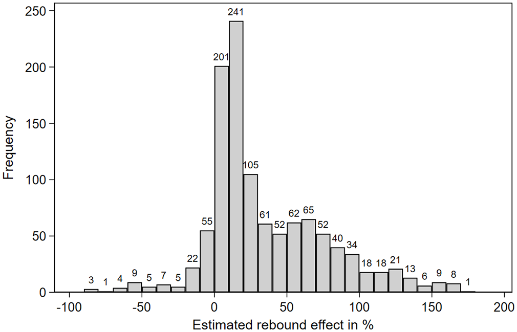
Histogram of rebound estimates (excluding outliers).

The summary statistics (Table 1) confirm the large variation in rebound estimates both across and within moderator categories.⁹ For the moderator impact, for example, we document mean rebound estimates ranging from 18% (CO₂) to 97% (social indicator). Similarly, there are differences in rebound estimates related to the assumed direct rebound, that is, studies assuming 0% to 20% direct rebound report a total rebound of 27% on average, while studies assuming 60% to 90% direct rebound report 106% total rebound on average.

Table 1.

Summary Statistics—Rebound Estimates by Selected Categorical Moderators.

Categorical moderators	N	Mean	Std. Dev.	Min	Max
Total	1118	35.01	41.45	−86.20	170.11
Rebound scenario setup
Type of action
Behav. change/sufficiency	260	45.19	42.57	−73.00	159.00
Efficiency improvement	829	31.39	40.22	−86.20	170.11
Both	29	47.09	49.54	−51.00	147.00
Area of action
Residential energy	614	31.42	40.43	−86.20	170.11
Food	111	43.65	43.12	−68.00	152.90
Transport/travel	242	33.59	38.02	−58.00	159.00
Other	65	68.64	55.49	−73.00	154.00
Multiple	86	28.02	29.29	1.70	154.12
Rebound impact measure
CO₂	264	17.69	37.27	−86.20	170.11
CO₂-eq	468	27.59	33.21	−73.00	159.00
Energy	248	58.32	43.15	−56.40	165.21
Social indicator	16	97.26	15.34	68.00	128.00
Total material requirement	29	49.86	38.91	5.00	153.00
Other env. indicator	93	43.95	48.62	−6.70	167.26
Rebound by income group
Average income	953	35.53	43.17	−86.20	170.11
High income	82	27.18	25.10	4.70	111.84
Low income	83	36.70	32.93	−5.50	131.20
Rebound estimation
Re-spending scenario type
Proportional	324	51.75	45.24	−73.00	167.26
Marginal	625	26.12	34.50	−86.20	170.11
Hypothetical: Green case	56	42.25	48.13	−64.00	162.00
Hypothetical: Worst case	6	105.76	45.01	55.29	155.00
Other	107	28.45	43.48	−68.00	159.00
Level of direct rebound assumed
Not assumed	904	28.93	38.87	−86.20	170.11
0%–20%	57	27.30	25.86	3.48	167.26
30%–50%	124	63.84	38.03	1.67	165.21
60%–90%	33	106.46	31.07	60.00	165.00

As specific subsamples may have otherwise unobserved characteristics, we inspect observations from three different categorical moderator levels more closely. The chosen subsamples reflect important dimensions linked to the general setup of the rebound scenario, that is, efficiency improvement (type of action), residential energy (area of action), and energy (rebound impact measure), and provide a sufficient number of observations to allow for subsequent analyses.

4.2 Regression Results

The results of the meta-regression are reported in Table 2 containing results for the whole sample and the three subsamples (efficiency improvement (type of action), residential energy (area of action), and energy (rebound impact measure)). In line with our methodological setup, we use the standard multivariate model as our baseline regression in column (1) and report results of alternative specifications in columns (2) to (4).¹⁰ In columns (5) to (7), we additionally present results for the three relevant subsamples identified in Section “Summary Statistics.” In all cases, we use the previously defined set of core moderators and exclude outliers based on the IQR, as explained above. Our description of the regression results focuses on the results of the baseline regression (column (1)) and points to the alternative specifications only in case of distinct differences. A series of robustness checks including additional moderators, different definitions of outliers and trimmed datasets is discussed in section “Robustness Checks.”

Table 2.

Regression Results.

Main	Baseline	Alternative specifications			Subsamples
	(1)	(2)	(3)	(4)	(5)	(6)	(7)
	Baseline	Baseline weighted	Random effects	Fixed effects	Efficiency	Residential energy	Impact: Energy
Mean total rebound effect (constant)	50.22^*** (7.97)	51.73^*** (9.41)	49.22^*** (9.41)	40.75^*** (12.18)	48.08^*** (7.06)	40.67^*** (6.13)	53.81^*** (8.31)
Data
HH consumption data is from expenditure survey	−1.80 (6.20)	8.96 (7.05)	−3.63 (8.79)		−4.00 (6.39)	−5.32 (4.94)	−31.40 (22.77)
Impact measure data not from input-output tables	−39.08^*** (13.78)	−60.18^*** (17.36)	−46.06^*** (13.97)		−38.17^*** (12.94)	−28.29^*** (8.45)	−69.68 (46.01)
Life-cycle assessment data used	−13.04^** (5.56)	−14.15^** (6.15)	−11.25^** (5.13)	−7.09 (6.36)	−14.23^** (6.15)	−3.62 (5.33)	−16.96^*** (4.73)
Rebound scenario setup
Type of action (ref. Efficiency)
Behav. change/sufficiency	17.14^*** (5.76)	4.25 (7.35)	24.13^*** (6.15)	26.86^*** (6.42)		17.65^*** (6.38)	16.12 (19.91)
Both	11.76 (10.84)	−11.91 (13.99)	35.87^*** (6.56)	41.07^*** (7.04)		−5.37 (5.21)	7.45 (9.41)
Area of action (ref. Residential energy)
Food	11.54 (10.32)	6.71 (10.22)	5.43 (12.80)	6.53 (14.49)			77.39^*** (7.33)
Transport/travel	25.93^*** (8.10)	24.54^*** (8.62)	16.63^** (7.88)	16.02^* (8.19)	28.29^*** (8.58)		20.22 (15.28)
Other	45.43^*** (7.79)	54.20^*** (13.94)	42.75^*** (9.40)	41.61^*** (9.50)	17.41 (35.80)		93.98^*** (8.44)
Multiple	8.84 (5.60)	3.17 (9.83)	5.84 (3.57)	5.35 (3.31)	6.90 (6.28)		20.77 (11.96)
Rebound impact measure (ref. Energy)
CO₂	−10.78 (8.94)	−13.90 (8.46)	−9.15 (9.61)	−13.38 (13.18)	−8.37 (8.11)	−9.75^* (4.84)
CO₂-eq	−23.72^** (8.93)	−20.26^** (7.92)	−16.92 (11.70)	−16.08 (14.38)	−20.66^** (8.34)	−18.28^** (7.12)
Social indicator	44.20^*** (7.62)	28.41^*** (8.83)	31.76^*** (9.37)	31.72^*** (10.55)	58.54^*** (14.03)	69.81^*** (4.49)
Total material requirement	.58 (9.75)	2.29 (10.17)	−8.82 (9.90)	−7.54 (9.12)	13.54^* (6.96)	6.23 (6.40)
Other env. indicator	−9.23 (10.04)	−2.98 (11.86)	−5.40 (10.68)	−5.49 (12.76)	13.33^* (7.64)	16.10^*** (5.72)
Rebound by income group (ref. Average income)
High income	5.04 (4.66)	4.16 (5.78)	−2.15^** (1.00)	−3.28^*** (1.09)	4.43 (4.60)	5.38 (4.71)	−7.84^*** (1.92)
Low income	14.53^** (6.67)	19.81^** (7.44)	7.05^** (2.90)	5.88^** (2.59)	9.25^* (4.81)	10.20^* (5.81)	12.05^*** (2.84)
Efficiency costly	−21.29^*** (7.71)	−22.15^** (9.27)	−10.76^** (4.70)	−5.82 (4.80)	−20.53^** (8.10)	−11.46^*** (2.61)	−2.64 (21.18)
Embodied resources considered	20.20^** (9.18)	17.40 (13.29)	2.24 (3.65)	−2.58 (4.98)	21.01^** (9.71)	5.18 (3.83)
Rebound estimation
Substitution and income effect	20.58 (12.55)	48.35^*** (14.31)	15.62^** (7.34)	12.11^** (5.72)	19.68^* (11.31)	2.29 (6.61)	43.30^*** (5.94)
Rebound is indirect only	−18.34^*** (5.46)	−19.93^*** (4.73)	−19.96^*** (5.98)	−20.42^*** (6.14)	−19.81^*** (6.74)	−25.16^*** (7.21)	−30.93^*** (3.84)
Re-spending scenario type (ref. Marginal)
Proportional	−10.73 (6.97)	2.38 (7.02)	−2.77 (2.81)	−3.37 (2.14)	−6.21 (6.07)	.58 (4.93)	−6.80^** (3.11)
Hypothetical: Green case	−20.14^*** (5.89)	−5.72 (7.23)	−12.76^*** (2.99)	−12.85^*** (2.75)	−14.51^* (7.36)	−4.35 (5.58)	−12.78^*** (3.49)
Hypothetical: Worst case	52.52^*** (14.57)	64.31^*** (18.59)	46.00^*** (12.18)	46.48^*** (10.95)	59.24^*** (21.14)	66.46^*** (20.14)	46.72^*** (7.97)
Other	−2.82 (7.97)	2.97 (7.44)	2.30 (3.22)	2.30 (2.83)	−1.30 (9.20)	5.51 (5.23)	−6.90 (5.23)
Estimation of an Almost Ideal Demand System	−16.62^** (7.36)	−13.81^* (7.29)	−.36 (9.85)	.00 (.)	−16.88^* (8.47)	−.73 (4.39)	10.30 (22.35)
Level of direct rebound assumed (ref. Not assumed)
0%–20%	10.34 (7.57)	−4.04 (10.04)	−3.63 (5.55)	−5.33 (5.73)	8.90 (7.09)	9.29 (6.59)	5.97 (8.43)
30%–50%	33.46^*** (6.66)	24.42^*** (8.43)	24.87^*** (5.69)	21.31^*** (7.44)	30.85^*** (5.29)	34.05^*** (5.29)	30.71^*** (8.43)
60%–90%	72.73^*** (7.49)	55.80^*** (8.75)	57.59^*** (9.68)	54.57^*** (11.06)	70.18^*** (9.30)	72.00^*** (11.61)	74.02^*** (10.67)
Observations	1118	1118	1118	1118	829	614	248
R²	.451	.508	.392	.265	.555	.628	.615
Adjusted R²	.437	.495		.248	.541	.612	.577

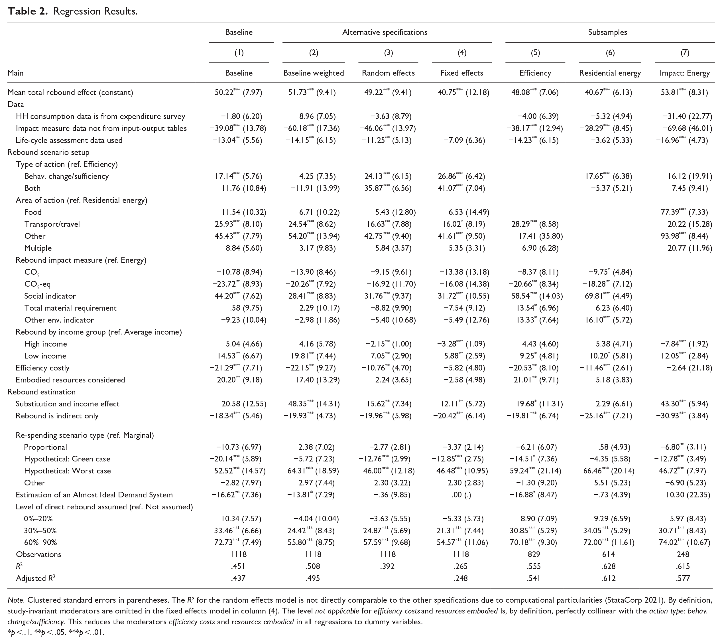
Note. Clustered standard errors in parentheses. The R² for the random effects model is not directly comparable to the other specifications due to computational particularities (StataCorp 2021). By definition, study-invariant moderators are omitted in the fixed effects model in column (4). The level not applicable for efficiency costs and resources embodied Is, by definition, perfectly collinear with the action type: behav. change/sufficiency. This reduces the moderators efficiency costs and resources embodied in all regressions to dummy variables.

p < .1. **p < .05. ***p < .01.

Turning to the results, we tested the baseline model for normality of residuals, influential observations, heteroscedasticity and multicollinearity (see also Figure A3 in Appendix A). The findings support inference validity but indicate heteroscedasticity, which we address using standard errors clustered at the study level. Multicollinearity did not influence the regression results in any relevant way.¹¹

As the core moderators are exclusively binary or categorical variables, their corresponding coefficients represent the expected change in mean total rebound induced by a deviation from the reference case (ceteris paribus). For all categorical moderators, the reference case is the omitted category indicated in parentheses. The reference case for all binary regressors is the zero case.¹² Accordingly, the constant mirrors the mean total microeconomic rebound for a reference study. It is neither a mere literature-wide nor an economy-wide average. Instead, it reflects the average rebound effect given the specification of the moderators, which capture both study design and rebound scenarios under consideration. We chose our reference cases for the respective variables such that they form a relevant combination of design choices frequently used in the primary studies. This consistent baseline avoids incongruous combinations like, for example, a sufficiency related action and the estimation of substitution effects (cf. Online Appendix A). The reference study in the meta-regressions displayed in Table 2 employs, for example, aggregate household expenditure data, impact data from input-output tables and a marginal re-spending scenario to estimate a total microeconomic rebound effect in terms of energy following an efficiency improvement in residential energy use.

The estimated mean total rebound is rather stable across specifications with little variance, ranging between 41% and 52% for our specifications presented in Table 2, columns (1) to (4). The adjusted R² varies between 0.248 and 0.495, which is a common range for meta-analyses on heterogeneous studies (Dimitropoulos, Oueslati and Sintek 2018; Mattmann, Logar and Brouwer 2016; Schütt 2021). In the following, we present results by moderator category starting with the type of data a study used.

4.2.1. Data

The source of household consumption data does not seem to affect the size of the rebound effect. Apparently, using data from household expenditure surveys instead of aggregated household data does not lead to differences in the estimated size of the rebound effect. Furthermore, the estimated rebound effect is significantly smaller (39 percentage points in the baseline specification) if the information for impact measures was not derived from input-output tables but rather carbon intensities or direct energy use and efficiency databases. This is due to only 76 observations in that category originating from three studies with particular characteristics, which we address in the discussion in Section “Discussion and Conclusion.” Additionally, using LCA data results in significantly smaller estimates of rebound effects (13 percentage points in the baseline specification).

4.2.2. Rebound Scenario Setup

Behavioral changes generally result in higher rebound effects compared to efficiency related actions. Additionally, the area of action considered by a study partly affects the size of the rebound effect. While the rebound effect for some areas of action (residential energy, food, multiple areas) do not differ significantly, the rebound effect for transport or travel related actions are larger than actions related to residential energy.¹³ Moreover, the choice of the rebound impact measure has a sizeable impact on the estimated rebound effect. Using CO₂-eq instead of energy reduces the mean effect size by about 20 percentage points albeit not significantly so in some specifications. If a social indicator such as employment hours is used instead, the rebound effect almost doubles in some specifications compared to rebound effects with energy as impact measure. The corresponding coefficient however, is based on only sixteen observations, implying limited informative value. Turning to the differences between income groups, we find that low income levels are associated with higher rebound effects, which is consistent with the findings of individual studies investigating this matter (e.g., Chitnis et al. 2014; Hagedorn and Wilts 2019; Murray 2013). Rebound effects for high income levels, on the other hand, are not significantly different from the average income levels in most specifications. This may be due to the few observations from high income groups and the coefficients’ relatively small magnitude. If the costs of an efficiency increase are considered in the rebound scenario, the resulting rebound effect is considerably smaller (21 percentage points in the baseline specification). This reflects the smaller amount of money that can be re-spent on other goods and services compared to a situation in which an efficiency increase is assumed to be costless. Additionally, if the respective resources embodied in the production and supply of an energy efficiency measure are accounted for, the estimated rebound effect increases accordingly, albeit significantly only in the baseline specification and in the efficiency subsample (models (1) and (5)).

4.2.3. Rebound Estimation

Studies that consider substitution effects in addition to income effects report larger rebound effects, and to a significant extent in almost all specifications. As expected, studies that only estimate an indirect rebound effect, show smaller effect sizes on average. The mean rebound effect is reduced by more than a third in the baseline specification.¹⁴ Furthermore, the re-spending scenario type seems to have a large impact on the size of the rebound. While there is no significant difference between the two types of data-based re-spending scenarios (proportional and marginal), hypothetical re-spending scenarios result in significantly different rebound estimates in most cases. This is, at least partly, by design. Assuming a worst case scenario, i.e., entire re-spending on a good or sector(s) with the highest impact, significantly increases the estimated rebound by a factor of more than two. In contrast, assuming a green case scenario, that is, re-spending with the least adverse impact reduces the estimated rebound in most specifications. The occasional insignificance may be due to the fact that there are only fifty-six observations with a green case scenario stemming from six studies. Within the marginal spending category, studies estimating an Almost Ideal Demand System to derive elasticities tend to report smaller rebound effects on average, though this effect is statistically significant only in the baseline specification. Finally, another important methodological choice of the studies is the assumption of a direct rebound effect. As expected, studies that assume a high direct rebound effect also report a significantly higher total rebound effect. The higher the assumed direct rebound, the larger the effect, and it turns insignificant at the smallest level (0%–20% assumed direct rebound effect).

4.3 Robustness Checks

We assess the robustness of our results in several ways. First, we split the sample in three above identified subsamples (efficiency improvement (type of action), residential energy (area of action), and energy (rebound impact measure)), depicted in columns (5) to (7) of Table 2. Second, we add hitherto unused moderators to the baseline specification, see Table A2 in Appendix A. Finally, we investigate the sensitivity of results to our definition of outliers, treatment of heteroscedasticity, and the effect of coding decisions as summarized in Table A3 in Appendix A.

In general, the subsample analyses depicted in Table 2 confirm the findings from the regression results based on the full sample. However, there are minor differences. Noticeably, the adjusted R² increases for all subsamples, now ranging between 0.541 and 0.612. This increase in explanatory power reflects the increased homogeneity of the analyzed sample. The subsamples on efficiency related actions (5) and rebounds in the residential energy area (6) lead to virtually identical results. In contrast, for the subsample of rebound effects measured in terms of energy (7), two previously insignificant moderators become significant (area of action: food and re-spending scenario type: proportional), while three others lose significance (impact measure data not from input-output tables, type of action: behav. change/sufficiency, and efficiency costly). We attribute these differences to the much smaller sample size of only 248 observations compared to the full sample with 1,118 observations and the other two subsamples with 829 and 614 observations, respectively. Notably, the smaller sample size goes along with fewer observations per level in the affected moderators. For example, the number of cases in which the costs of efficiency improvements are accounted for decreases from 260 in the full sample to 20 in this subsample.

Similarly, adding moderators does not alter results considerably (see Table A2 in Online Appendix B). First, both the explanatory power in terms of R² and the coefficients of the core moderators remain stable. Second, most of the added moderators are insignificant, that is, adding information on whether only direct emissions are considered (3), the year of publication (4), or whether the study was published in a peer-reviewed journal (5) has no significant effect. Adding a dummy variable controlling whether a detailed efficiency or sufficiency change scenario is used (2) yields an effect that is only a weakly significant at the 10% level. When controlling for author group effects (6), some minor differences emerge that accordingly result in an altered mean rebound effect due to the change in the baseline.

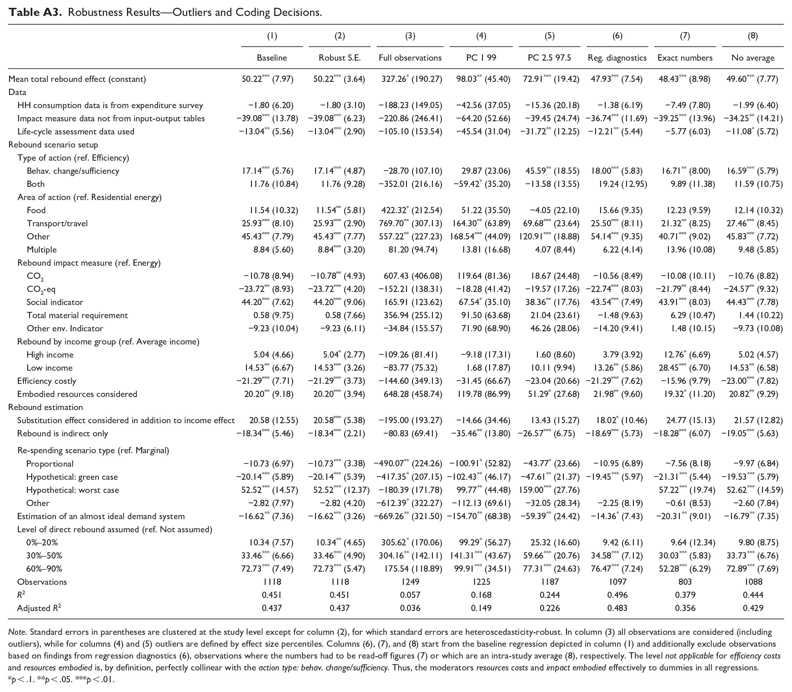
Finally, we investigate if our outlier specification or coding decisions have an effect on the results (Table A3 in Appendix A). We first assess if our decision to cluster standard errors at the study level is too restrictive, thus resulting in overly narrow confidence intervals. The use of common heteroscedasticity-robust standard errors (2) instead confirms the insights gained from the baseline specification.¹⁵ Similarly, assessing the effect of outliers supports our decision to omit extreme rebound effect estimates using the IQR in our main specifications. First, using all available observations clearly distorts the regression results (column (3)), while regressions with fewer extreme rebound estimates (using different percentile ranges) improve in explanatory power and have more reasonable coefficient magnitudes (columns (4) and (5)). However, omitting even more observations based on the regression diagnostics (6) does not alter the baseline results such that the IQR appears to be a justified outlier criterion. Finally, our coding decisions, that is, reading numbers off figures (7) and using intra-study averages if necessary (8), did not affect the results noticeably.

5. Transfer Reliability

This meta-analysis on microeconomic rebounds primarily serves to explain heterogeneous empirical findings and calculate mean effect sizes relative to our consistent baseline scenario.¹⁶ As an addition, we assess the usefulness of the results of our meta-regression analysis in new policy contexts by calculating transfer errors (Chaikumbung, Doucouliagos and Scarborough 2016). This is particularly important in the context of rebound effects, where estimation is data and time intensive and thus costly, posing a burden on primary studies (Johnston et al. 2015).

We follow common practice and calculate absolute percentage errors (APE) using leave-one-out-cross-validation, that is, we omit one observation at a time, re-estimate the model, and calculate the estimated APE for the observation omitted (Chaikumbung, Doucouliagos and Scarborough 2016; Johnston, Rolfe and Zawojska 2018; Nelson 2015). Additionally, we show the corresponding absolute errors (AE), which presumably better reflect the expected predictive accuracy of our meta-model as explained below.

In Table 3, we present the APE and AE for the baseline specification (Full sample) as well as for the subsamples of rebound effect sizes related to efficiency improvements (type of action), residential energy (area of action), and energy (rebound impact measure), respectively. We base the calculation of these error matrices on a meta-functional transfer using the respective regression results from Table 2, which is common practice (Johnston et al. 2015; Kaul et al. 2013).¹⁷

Table 3.

Transfer Errors.

	N	Mean (SD)	Median	Range
Absolute percentage error (APE)
Full sample	1,092	297.86 (1829.56)	52.50	0.41–44, 090
Efficiency	821	224.63 (1741.49)	50.57	0.04–43, 226
Residential energy	607	193.92 (1451.27)	48.42	0.09–33, 285
Energy	248	105.34 (258.76)	31.32	0.00–2, 739
Absolute error (in percentage points)
Full sample	1,118	22.55 (22.19)	15.78	0.07–150
Efficiency	829	18.97 (20.54)	11.70	0.01–130
Residential energy	614	17.59 (18.64)	10.92	0.01–142
Energy	248	21.95 (19.22)	16.64	0.00–116

Note. The number of observations for the APE is smaller compared to the AE in some cases since twenty-five observations have a reported rebound of 0% which prohibits the calculation of a percentage transfer error (APE). Additionally, one observation with an extreme APE (3.96¹⁵%) is omitted which reduces the Mean APE from 3.62¹²% to 298% for the full sample, while the median APE barely changes.

The general findings from Table 3 are consistent with previous discussions in the literature. First, transfer errors are smaller for more homogeneous sets of observations (i.e., our subsamples). Second, the mean transfer error is larger than the median transfer error regardless of the metric due to a few outlying observations. More specifically, the mean APE ranges between 105% and 298% compared to 31% and 53% for the median APE. In particular, extremely high APE values correspond exclusively to rebound estimates that are close to zero. In these cases, relatively small absolute errors lead to high percentage errors. This pattern is also documented in Figure 2, which shows the distribution of APEs.¹⁸ Arguably, the median APEs in this case better capture the expected APE.

Figure 2.

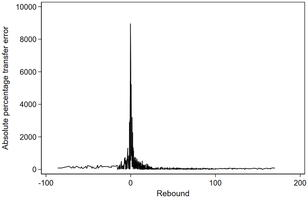
Absolute transfer error (%) by rebound.

Hence, for policy makers, the AE is presumably a more informative metric to assess transfer accuracy, as it conveys a direct indication of the expected rebound magnitude. In general, the AE is relatively small with a mean of 23 percentage points and a corresponding median of 16 for the full sample. For the subsample of rebound estimates related to residential energy, the mean and median AE even reduce to approximately 18 and 11 percentage points, respectively. Therefore, it appears that our meta-analytic model reliably forecasts the expected rebound on average, notwithstanding a few extreme cases.

We are aware that our analysis cannot provide detailed guidance for a specific policy. Rather, we provide an indication of the general effect sizes for a variety of policy areas that could serve as a basis for more detailed investigation. Taking the EU’s energy efficiency targets as an example, Member States are required to regularly publish National Energy and Climate Plans (NECP) which contain national energy efficiency targets and lay out concrete measures how to achieve them, underpinned by explicit calculations of expected energy savings (EU 2018/1999). As there is no unified calculation framework for all sectors and types of measures, Member States have to develop their own methodologies for calculating energy savings. For example, while the German NECP explicitly takes rebound effects into account and adjusts gross to net savings per measure (cf. German final NECP, p. 225), other NECPS neither mention the possibility of rebounds nor explicitly adjust for them (e.g., Italian, French, and Spanish NECPs¹⁹). Such omissions are at odds with the microeconomic rebound literature and our meta-analysis thereof. As our results show, rebound effects must indeed be expected to considerably decrease the effectiveness of energy efficiency improvements and sufficiency-related behavioral changes to reduce resource use. Hence, policy-makers should be encouraged to perform detailed analysis of rebound effects accompanying specific policy measures. Our results might serve as a starting point in this respect. Additionally, measures to assess the national, economy-wide rebound effect of implementing, for example, all the policy measures in a NECP should be developed. While such endeavors lie outside the scope of the literature analyzed here and thus our meta-analysis, Borenstein (2015) has discussed the potential use of a macroeconomic multiplier to scale up microeconomic rebound effects and Heun, Semieniuk and Brockway (2022) have introduced the first operationalization of this concept. Future research should further explore this link and develop methods to aggregate microeconomic rebound effects of individual policy measures.

6. Discussion and Conclusion

Information on rebound effects is essential to account for unintended consequences of policies for the sustainable use of natural resources and to achieve governments’ ambitious targets such as decarbonization targets. Due to the importance of evaluating how effective a particular policy measure might be, a relatively large literature exists on estimating rebound effects. Unfortunately, the effect sizes of quantified rebound effects vary widely, ranging from negative values to above 100%, requiring a systematic assessment of the causes for the heterogeneity of empirical results. In this paper, we conducted a meta-analysis of the literature, focusing on studies that estimated total microeconomic rebound effects on the household level. We identified forty-three studies published between 2002 and 2020 that provided us with 1,118 observations with rebound estimates ranging from −86% to 170% (after outlier exclusion). While the overall distribution of rebound effects (shown in Figure 1) might appear to indicate that rebound effects are predominantly small, our detailed analysis shows that the assumption of an overall low mean or modal rebound would be grossly misleading, as there are significant differences across several dimensions. In our meta-regression analysis, we identified a rich set of moderators that represent relevant dimensions in which studies differ. These consist of: (1) type of data sources, (2) setup of the rebound scenario (e.g., type and area of action, rebound impact measure), and (3) type of rebound estimation (e.g., re-spending scenario type, level of direct rebound assumed). In the following, we highlight a few results, relevant for decision makers when assessing the effectiveness of future decarbonization policies based on existing literature and for researchers when designing future rebound studies.

For our reference case, we find a mean total rebound effect between 41% and 52%, that is, a total microeconomic rebound effect in terms of energy following an efficiency improvement in residential energy use. Of the three variables in our first moderator dimension, that is, type of data sources, both the dummy variable indicating that the impact measure data is not derived from IO tables and the dummy variable indicating that LCA data has been used exhibit a statistically and economically significant negative effect. While the effect of the latter is moderate (−13 percentage points in the baseline specification), the use of non-IO data has a considerably larger effect (−39 percentage points in the baseline specification). It is worth noting here that there are only three studies (with a total of 76 observations) that do not employ IO data: Chitnis, Fouquet and Sorrell (2020) and Kratena and Wüger (2010) employ direct CO₂ emissions and direct energy databases, respectively, whereas Zhang et al. (2017) use a database of both direct and embedded CO₂ emissions. As we do not find a statistically significant effect of the variable only direct emissions considered (cf. Table A2 in Appendix A), we can rule out this common feature of two out of the three studies as the driver of the effect. Apart from that, we have to be somewhat cautious when interpreting the effect. It may be due to the data sources for the impact measure as such, but also to finer details in study design that our moderators cannot capture as they are rare in our dataset. For example, Kratena and Wüger (2010) focus on modelling interdependencies between the energy efficiency of the stock of household appliances and rebound effects and Chitnis, Fouquet and Sorrell (2020) provide the only estimates of rebound effects between energy services (e.g., cooking) rather than energy commodities (e.g., electricity).

Turning to the second moderator dimension, we find that the setup of the rebound scenario significantly impacts the size of the estimated rebound effect across several moderators. Rebound effects preceded by sufficiency-related behavioral changes are on average 17 percentage points higher than rebound effects preceded by efficiency improvements. Surprisingly, this difference between efficiency and sufficiency actions is not mitigated by controlling for whether the costs of and resources embodied in efficiency improvements are accounted for in the rebound scenario under consideration. The first of these moderators, that is, efficiency costly, yields the expected negative effect as spending on energy efficiency measures reduces monetary savings and thus the budget available for re-spending and, consequently, the rebound effect. The second relevant moderator, that is, resources embodied, in turn yields the expected positive effect as accounting for the resources embodied in energy efficiency measures rather than just the resources embodied in other goods and services will increase the rebound effect. This effect is, however, only statistically significant in the baseline specification and the efficiency subsample. Hence, while we can rule out these two differences between efficiency actions which tend to be associated with costs and embodied resource use and sufficiency actions which are typically not, further research will be required to explain the finding that—even when controlling for the costs and embodied resource use of efficiency measures—sufficiency-related behavioral changes induce higher rebound effects.

In terms of the consumption area in which the efficiency or sufficiency actions take place, actions in the transport area lead to rebound effects that are on average 26 percentage points higher than actions in the area of residential energy. This is of crucial importance for policy makers who should account for higher rebound effects when preparing and evaluating future policies in the transport sector as compared to the residential energy sector. Policy makers should also be aware that the size of the expected rebound effect depends on the impact measure. Presumably due to the close link between energy generation and CO₂ emissions, we do not find a difference in rebound effects in terms of these two impact measures. We do, however, find rebound effects in terms of CO₂-eq, that is, including other GHG like methane and nitrous oxide which are less closely linked to energy generation, to be on average 24 percentage points lower than rebound effects in terms of energy. In terms of rebound effects by income groups, our analysis confirms the consensus in the literature that rebound effects are significantly higher for low-income households (15 percentage points higher than in the average income group). The effect for high-income groups is small and statistically significantly negative in only three of our seven main models, suggesting that the difference between high- and average-income households in terms of rebound effects is less pronounced than the difference between low- and average-income households.

Our final group of moderators includes those that describe the rebound estimation as such, that is, which components of the total microeconomic rebound effect are estimated, how households’ re-spending is modeled and whether direct rebound effects are assumed. Unsurprisingly, most of these factors have a strong influence on the estimated rebound effects with the effects having the expected signs. The only exception is that we do not find a significant difference between the two data-based re-spending types, that is, marginal and proportional re-spending. Hence, whether or not changes in households’ expenditure shares due to changes in income are accounted for has no direct impact on the size of the estimated rebound effect. However, two variables closely related to the marginal spending case are significant and have to be considered here. First, a subset of the studies employing marginal spending apply an Almost Ideal Demand System to estimate marginal budget shares or elasticities. We find the application of an Almost Ideal Demand System to result in rebound effects that are on average 17 percentage points smaller than rebound effects that are calculated employing marginal spending but no demand system estimation. It should be noted though that this effect is less stable across specifications than most of the other effects discussed here, as the baseline specification is the only one in which it is significant at the five percent level. We therefore refrain from any definitive conclusions. Second, a subset of the studies applying an Almost Ideal Demand System estimate not only income or expenditure elasticities but also own- and cross-price elasticities. The latter are necessary prerequisites for the estimation of substitution effects. The inclusion of these effects as opposed to considering income effects alone in turn leads to significantly higher rebound estimates and should thus not be neglected when estimating efficiency rebounds.²⁰ Furthermore, it would be desirable for there to be not only more applications of fully fledged demand system but also more discussions on how to best adapt demand systems for the estimation of rebound effects. For example, Schmitz and Madlener (2020) explicitly include energy efficiency in their demand system estimation. The case of sufficiency rebounds is, of course, different. There are no price changes and, consequently, no substitution effects to consider. Furthermore, sufficiency-related behavioral changes are somewhat removed from classical economic theory, which raises the question of how to realistically describe the re-spending of households that have made such changes. Few studies explore green case and worst case re-spending scenarios and the microeconomic literature hardly considers theories and empirical results concerning spill-over effects and moral licensing from the psychological literature (cf. Dütschke et al. 2018; Reimers, Lasarov and Hoffmann 2022; Sorrell, Gatersleben and Druckman 2020).

In conclusion, considerations of internal consistency of the setup of the rebound scenario and the estimation approach are important both in interpreting our results and in designing future studies quantifying rebounds. The current state of the rebound literature is characterized by a wide variation in terms of the level of detail and specification of rebound scenarios, which makes it challenging to find moderators that can be meaningfully coded for all studies or at least within subsamples of studies. Given these circumstances, our moderators explain a substantial share of the variation in rebound estimates. Specifically, our results are most informative and reliable where they concern commonly studied rebound scenarios. For non-standard data sources, areas of action and impact measures that have so far only been studied in very few cases, we have to rely on catch-all categories with few observations. Further differentiation and thereby more meaningful interpretations for these categories will only become possible as the number of primary studies investigating them increases. We thus hope that future studies advancing the empirical methodology for quantifying microeconomic rebound effects will allow for more detailed (meta-) analyses. Nevertheless, our meta-analysis already allows for reliable conclusions. In terms of predictive accuracy, we find that our meta-regression model results in relatively small absolute error margins (about 20 percentage points).

As stated in the introduction, the broad applicability and relevance of the rebound concept has led to the development of a diverse literature. That being the case, it is important to note that our meta-regression analysis is concerned with a specific sub-section within the broader rebound literature with many studies falling out of our scope, for example, due to considering the firm rather than the household level, focusing exclusively on direct or on economy-wide rebound effects or applying (quasi-)experimental methods. We thus hope that future meta-regression analyses will take on other strands of the rebound research, making use of meta-regression analysis not only as a powerful tool to summarize and guide the progress within the different strands of rebound research but also to aid their integration.

Supplemental Material

sj-docx-1-enj-10.1177_01956574241289004 – Supplemental material for How to Explain the Huge Differences in Rebound Estimates: A Meta-Regression Analysis of the Literature

Supplemental material, sj-docx-1-enj-10.1177_01956574241289004 for How to Explain the Huge Differences in Rebound Estimates: A Meta-Regression Analysis of the Literature by Marvin Schütt, Anke Jacksohn, Tobias Möllney and Katrin Rehdanz in The Energy Journal

Footnotes

Appendix A: Tables and Figures

Table A3.

Robustness Results—Outliers and Coding Decisions.

	(1)	(2)	(3)	(4)	(5)	(6)	(7)	(8)
	Baseline	Robust S.E.	Full observations	PC 1 99	PC 2.5 97.5	Reg. diagnostics	Exact numbers	No average
Mean total rebound effect (constant)	50.22^*** (7.97)	50.22^*** (3.64)	327.26^* (190.27)	98.03^** (45.40)	72.91^*** (19.42)	47.93^*** (7.54)	48.43^*** (8.98)	49.60^*** (7.77)
Data
HH consumption data is from expenditure survey	−1.80 (6.20)	−1.80 (3.10)	−188.23 (149.05)	−42.56 (37.05)	−15.36 (20.18)	−1.38 (6.19)	−7.49 (7.80)	−1.99 (6.40)
Impact measure data not from input-output tables	−39.08^*** (13.78)	−39.08^*** (6.23)	−220.86 (246.41)	−64.20 (52.66)	−39.45 (24.74)	−36.74^*** (11.69)	−39.25^*** (13.96)	−34.25^** (14.21)
Life-cycle assessment data used	−13.04^** (5.56)	−13.04^*** (2.90)	−105.10 (153.54)	−45.54 (31.04)	−31.72^** (12.25)	−12.21^** (5.44)	−5.77 (6.03)	−11.08^* (5.72)
Rebound scenario setup
Type of action (ref. Efficiency)
Behav. change/sufficiency	17.14^*** (5.76)	17.14^*** (4.87)	−28.70 (107.10)	29.87 (23.06)	45.59^** (18.55)	18.00^*** (5.83)	16.71^** (8.00)	16.59^*** (5.79)
Both	11.76 (10.84)	11.76 (9.28)	−352.01 (216.16)	−59.42^* (35.20)	−13.58 (13.55)	19.24 (12.95)	9.89 (11.38)	11.59 (10.75)
Area of action (ref. Residential energy)
Food	11.54 (10.32)	11.54^** (5.81)	422.32^* (212.54)	51.22 (35.50)	−4.05 (22.10)	15.66 (9.35)	12.23 (9.59)	12.14 (10.32)
Transport/travel	25.93^*** (8.10)	25.93^*** (2.90)	769.70^** (307.13)	164.30^** (63.89)	69.68^*** (23.64)	25.50^*** (8.11)	21.32^** (8.25)	27.46^*** (8.45)
Other	45.43^*** (7.79)	45.43^*** (7.77)	557.22^** (227.23)	168.54^*** (44.09)	120.91^*** (18.88)	54.14^*** (9.35)	40.71^*** (9.02)	45.83^*** (7.72)
Multiple	8.84 (5.60)	8.84^*** (3.20)	81.20 (94.74)	13.81 (16.68)	4.07 (8.44)	6.22 (4.14)	13.96 (10.08)	9.48 (5.85)
Rebound impact measure (ref. Energy)
CO₂	−10.78 (8.94)	−10.78^** (4.93)	607.43 (406.08)	119.64 (81.36)	18.67 (24.48)	−10.56 (8.49)	−10.08 (10.11)	−10.76 (8.82)
CO₂-eq	−23.72^** (8.93)	−23.72^*** (4.20)	−152.21 (138.31)	−18.28 (41.42)	−19.57 (17.26)	−22.74^*** (8.03)	−21.79^** (8.44)	−24.57^** (9.32)
Social indicator	44.20^*** (7.62)	44.20^*** (9.06)	165.91 (123.62)	67.54^* (35.10)	38.36^** (17.76)	43.54^*** (7.49)	43.91^*** (8.03)	44.43^*** (7.78)
Total material requirement	0.58 (9.75)	0.58 (7.66)	356.94 (255.12)	91.50 (63.68)	21.04 (23.61)	−1.48 (9.63)	6.29 (10.47)	1.44 (10.22)
Other env. Indicator	−9.23 (10.04)	−9.23 (6.11)	−34.84 (155.57)	71.90 (68.90)	46.26 (28.06)	−14.20 (9.41)	1.48 (10.15)	−9.73 (10.08)
Rebound by income group (ref. Average income)
High income	5.04 (4.66)	5.04^* (2.77)	−109.26 (81.41)	−9.18 (17.31)	1.60 (8.60)	3.79 (3.92)	12.76^* (6.69)	5.02 (4.57)
Low income	14.53^** (6.67)	14.53^*** (3.26)	−83.77 (75.32)	1.68 (17.87)	10.11 (9.94)	13.26^** (5.86)	28.45^*** (6.70)	14.53^** (6.58)
Efficiency costly	−21.29^*** (7.71)	−21.29^*** (3.73)	−144.60 (349.13)	−31.45 (66.67)	−23.04 (20.66)	−21.29^*** (7.62)	−15.96 (9.79)	−23.00^*** (7.82)
Embodied resources considered	20.20^** (9.18)	20.20^*** (3.94)	648.28 (458.74)	119.78 (86.99)	51.29^* (27.68)	21.98^** (9.60)	19.32^* (11.20)	20.82^** (9.29)
Rebound estimation
Substitution effect considered in addition to income effect	20.58 (12.55)	20.58^*** (5.38)	−195.00 (193.27)	−14.66 (34.46)	13.43 (15.27)	18.02^* (10.46)	24.77 (15.13)	21.57 (12.82)
Rebound is indirect only	−18.34^*** (5.46)	−18.34^*** (2.21)	−80.83 (69.41)	−35.46^** (13.80)	−26.57^*** (6.75)	−18.69^*** (5.73)	−18.28^*** (6.07)	−19.05^*** (5.63)
Re-spending scenario type (ref. Marginal)
Proportional	−10.73 (6.97)	−10.73^*** (3.38)	−490.07^** (224.26)	−100.91^* (52.82)	−43.77^* (23.66)	−10.95 (6.89)	−7.56 (8.18)	−9.97 (6.84)
Hypothetical: green case	−20.14^*** (5.89)	−20.14^*** (5.39)	−417.35^* (207.15)	−102.43^** (46.17)	−47.61^** (21.37)	−19.45^*** (5.97)	−21.31^*** (5.44)	−19.53^*** (5.79)
Hypothetical: worst case	52.52^*** (14.57)	52.52^*** (12.37)	−180.39 (171.78)	99.77^** (44.48)	159.00^*** (27.76)		57.22^*** (19.74)	52.62^*** (14.59)
Other	−2.82 (7.97)	−2.82 (4.20)	−612.39^* (322.27)	−112.13 (69.61)	−32.05 (28.34)	−2.25 (8.19)	−0.61 (8.53)	−2.60 (7.84)
Estimation of an almost ideal demand system	−16.62^** (7.36)	−16.62^*** (3.26)	−669.26^** (321.50)	−154.70^** (68.38)	−59.39^** (24.42)	−14.36^* (7.43)	−20.31^** (9.01)	−16.79^** (7.35)
Level of direct rebound assumed (ref. Not assumed)
0%–20%	10.34 (7.57)	10.34^** (4.65)	305.62^* (170.06)	99.29^* (56.27)	25.32 (16.60)	9.42 (6.11)	9.64 (12.34)	9.80 (8.75)
30%–50%	33.46^*** (6.66)	33.46^*** (4.90)	304.16^** (142.11)	141.31^*** (43.67)	59.66^*** (20.76)	34.58^*** (7.12)	30.03^*** (5.83)	33.73^*** (6.76)
60%–90%	72.73^*** (7.49)	72.73^*** (5.47)	175.54 (118.89)	99.91^*** (34.51)	77.31^*** (24.63)	76.47^*** (7.24)	52.28^*** (6.29)	72.89^*** (7.69)
Observations	1118	1118	1249	1225	1187	1097	803	1088
R²	0.451	0.451	0.057	0.168	0.244	0.496	0.379	0.444
Adjusted R²	0.437	0.437	0.036	0.149	0.226	0.483	0.356	0.429

Note. Standard errors in parentheses are clustered at the study level except for column (2), for which standard errors are heteroscedasticity-robust. In column (3) all observations are considered (including outliers), while for columns (4) and (5) outliers are defined by effect size percentiles. Columns (6), (7), and (8) start from the baseline regression depicted in column (1) and additionally exclude observations based on findings from regression diagnostics (6), observations where the numbers had to be read-off figures (7) or which are an intra-study average (8), respectively. The level not applicable for efficiency costs and resources embodied is, by definition, perfectly collinear with the action type: behav. change/sufficiency. Thus, the moderators resources costs and impact embodied effectively to dummies in all regressions.

p < .1. **p < .05. ***p < .01.

Acknowledgements

We would like to thank the three anonymous reviewers for their valuable comments and suggestions on the earlier versions of this paper and Maike Schieferdecker for her excellent research assistance.

Declaration of Conflicting Interests

The author(s) declared no potential conflicts of interest with respect to the research, authorship, and/or publication of this article.

Funding

The author(s) disclosed receipt of the following financial support for the research, authorship, and/or publication of this article: This work was supported by the German Federal Ministry of Education and Research (BMBF) as a part of the iReliefs project (grant FKZ 01UT1706A).

Supplemental Material

Supplemental material for this article is available online.

1

The European Union’s (EU’s) Energy Efficiency , for example, sets an energy efficiency target for 2030 of at least 32.5% compared to projections of the expected energy use in 2030.

2

In most sufficiency scenarios direct rebound effects do not occur by definition. See for further details.

3

See Figure A1 and the associated text in for a detailed explanation of the total microeconomic rebound effect and its components.

4

The absence of precision measures is logical when proportional or hypothetical spending scenarios are applied and there is thus no estimation of elasticities or similar measures. When rebound effects are estimated based on marginal spending scenarios, it should generally be possible to report suitable measures. Yet, is the only study to do so, as the author reports confidence intervals for the estimated rebound effects.

5

The estimation of the population variability in effect sizes requires knowledge of the standard error ().

6

Using optimal inverse-variance weights would also ensure efficient estimation. Importantly, however, estimating equation (1) by OLS still ensures unbiased estimation even though efficiency may not be achieved ().

7

14 out of 43 studies included in this meta-analysis report negative rebound effects. We attribute the fact that there are fewer negative than positive rebound estimates in our sample to the rarely specified conditions that are necessary for negative rebounds to occur (i.e., very costly actions preceding the rebound effect that in turn reduce the available budget that can be re-spent on other goods and services or certain substitutionary and complementary relationships between and resource intensities of goods and services given that substitution effects are accounted for). We therefore conclude that a systematic under-reporting of negative rebound effects is unlikely.

8

Originally, 2343 separate estimates were coded (cf. column Orig. N in Table B3 in Online Appendix B). However, for two studies which reported values at the sub-national level (Chinese provinces) next to the national average, only the latter was ultimately kept (Chen et al. 2019; Wen et al. 2018). For consistency, for two additional studies which only reported values at the sub-national level, we aggregated the reported values to a GDP-weighted national average (Thomas, Hausfather and Azevedo 2014; ).

9

See Table A1 in for summary statistics of all moderators including those used for robustness checks.

10

The BPLM test indicated presence of additional study-level heterogeneity not accounted for by the standard multivariate model. However, both panel-model solutions have serious drawbacks: Using a REML has strong assumptions on the error term that unlikely hold in our case (Feld and Heckemeyer 2011) and using the FEML automatically omits study-invariant moderators from the regression that are of interest. However, the results are largely unaffected by the model choice, the moderators included already explain study-level heterogeneity to a high degree. In this setting, we prefer a parsimonious model and hence use the multivariate model presented in as a baseline for robustness checks and subsample analyses.

11

The mean variance inflation factor is 2.37. This is well below the usual threshold of 10, hence eliminating multicollinearity concerns.

12

In some of the robustness checks, we add continuous moderators to the model. These are centered to ease their coefficients’ interpretations as the effect of deviations from the mean.

13

Note that the category other is also significant. However, in this category we bundle sixty-five observations with very different action areas, for example, durable appliances, no chemicals & plastics, clothing, or paper. While aggregation in one category was necessary due to very few observations per action area, we refrain from drawing any conclusions accordingly.

14

Two studies in our sample estimate indirect rebound effects for efficiency scenarios under which direct rebound effects could be expected to occur, but are not accounted for in the analysis. Cellura et al. (2013) do not provide a specific reasoning for this approach. study rebound effects in smart homes and argue that the nudges provided by smart homes will prevent direct rebound effects from occurring. We have tried two different ways of coding the relevant cases, that is, we coded them as rebound indirect only = 1 and level of direct rebound not assumed and alternatively as rebound indirect only = 0 and level of direct rebound assumed = 0%–20%. The results are robust to these changes. The first variant is used throughout the paper.

15

This robustness check also addresses remaining concerns regarding the appropriateness of clustering the standard errors due to the moderate number of 43 studies serving as clusters ().

16

See our description of our baseline scenario in Section “Regression results.”

17

For completeness, we also calculated simple mean-value transfer errors based on a univariate analogue of equation (1). Results follow the same pattern (albeit with greater transfer errors as expected) and are accessible at .

18

Excluding rebound estimates between -1% and +1% (51 observations) reduces the mean APE from 298% to 125%, for example.

19

The NECPs for all EU member states are available at: . Last accessed 08.04.2024.

20

The significant positive effect is not present in our baseline regression but in most of the alternative specifications.

References

Alfredsson

Eva C.

2004. ““Green” Consumption—No Solution for Climate Change.” Energy 29 (4): 513–24. doi:10.1016/j.energy.2003.10.013.

Azevedo

Inês M. L.

2014. “Consumer End-Use Energy Efficiency and Rebound Effects.” Annual Review of Environment and Resources 39 (1): 393–418. doi:10.1146/annurev-environ-021913-153558.

Bardsley

Nicholas

Büchs

Milena

James

Patrick

Papafragkou

Anastasios

Rushby

Thomas

Saunders

Clare

Smith

Graham

Wallbridge

Rebecca

Woodman

Nicholas

. 2019. “Domestic Thermal Upgrades, Community Action and Energy Saving: A Three-Year Experimental Study of Prosperous Households.” Energy Policy 127: 475–85. doi:10.1016/j.enpol.2018.11.036.

Biewendt

Marcel

Blaschke

Florian

Böhnert

Arno

. 2020. “The Rebound Effect – A Systematic Review of the Current State of Affairs.” European Journal of Economics and Business Studies 6 (1): 106–20. doi:10.26417/134nvy47z.

Borenstein

Severin

. 2015. “A Microeconomic Framework for Evaluating Energy Efficiency Rebound and Some Implications.” The Energy Journal 36 (1): 1–21. doi:10.5547/01956574.36.1.1.

Briceno

Tanja

Peters

Glen

Solli

Christian

Hertwich.

Edgar G.

2005. “Using Life Cycle Approaches to Evaluate Sustainable Consumption Programs: Car-Sharing.” Working Papers 2/2005. http://hdl.handle.net/11250/242569.

Brockway

Paul E.

Saunders

Harry

Heun

Matthew K.

Foxon

Timothy J.

Steinberger

Julia K.

Barrett

John R.

Sorrell

Steve

. 2017. “Energy Rebound as a Potential Threat to a Low-Carbon Future: Findings From a New Exergy-Based National-Level Rebound Approach.” Energies 10 (1): 1–24. doi:10.3390/en10010051.

Brockway

Paul E.

Sorrell

Steve

Semieniuk

Gregor

Heun

Matthew K.

Court

Victor

. 2021. “Energy Efficiency and Economy-Wide Rebound Effects: A Review of the Evidence and Its Implications.” Renewable and Sustainable Energy Reviews 141: 110781. doi:10.1016/j.rser.2021.110781.

Brookes

Leonard

. 1979. “A Low-Energy Strategy for the UK by G. Leach et al: A Review and Reply.” Atom 269: 3–8.

10.

Buhl

Johannes

Acosta

José

. 2016. “Work Less, Do Less? Working Time Reductions and Rebound Effects.” Sustainability Science 11 (2): 261–76. doi:10.1007/s11625-015-0322-8.

11.

Card

Noel A

. 2012. Applied Meta-Analysis for Social Science Research. Methodology in the Social Sciences. New York: The Guilford Press. http://swb.eblib.com/patron/FullRecord.aspx?p=759913.

12.

Cellura

Maurizio

Di Gangi

Alessandra

Longo

Sonia

Orioli

Aldo

. 2013. “An Italian Input–Output Model for the Assessment of Energy and Environmental Benefits Arising From Retrofit Actions of Buildings.” Energy and Buildings 62 (2): 97–106. doi:10.1016/j.enbuild.2013.02.056.

13.

Chaikumbung

Mayula

Doucouliagos

Hristos

Scarborough

Helen

. 2016. “The Economic Value of Wetlands in Developing Countries: A Meta-Regression Analysis.” Ecological Economics 124:164–74. doi:10.1016/j.ecolecon.2016.01.022.

14.

Chan

Nathan W.

Gillingham

Kenneth

. 2015. “The Microeconomic Theory of the Rebound Effect and Its Welfare Implications.” Journal of the Association of Environmental and Resource Economists 2 (1): 133–59. doi:10.1086/680256.

15.

Chen

Zhenni

Huibin

Jianglong

Southworth

Frank

Shoufeng

. 2019. “Achieving Low-Carbon Urban Passenger Transport in China: Insights From the Heterogeneous Rebound Effect.” Energy Economics 81 (10): 1029–41. doi:10.1016/j.eneco.2019.06.009.

16.

Chitnis

Mona

Fouquet

Roger

Sorrell

Steve

. 2020. “Rebound Effects for Household Energy Services in the UK.” Energy Journal 41 (4): 31–59. doi:10.5547/01956574.41.4.mchi.

17.

Chitnis

Mona

Sorrell

Steve

. 2015. “Living Up to Expectations: Estimating Direct and Indirect Rebound Effects for UK Households.” Energy Economics 52: S100–16. doi:10.1016/j.eneco.2015.08.026.

18.

Chitnis

Mona

Sorrell

Steve

Druckman

Angela

Firth

Steven K.

Jackson

Tim

. 2013. “Turning Lights Into Flights: Estimating Direct and Indirect Rebound Effects for UK Households.” Energy Policy 55: 234–50. doi:10.1016/j.enpol.2012.12.008.

19.

Chitnis

Mona

Sorrell

Steve

Druckman

Angela

Firth

Steven K.

Jackson

Tim

. 2014. “Who Rebounds Most? Estimating Direct and Indirect Rebound Effects for Different UK Socioeconomic Groups.” Ecological Economics 106: 12–32. doi:10.1016/j.ecolecon.2014.07.003.

20.

Dimitropoulos

Alexandros

Oueslati

Walid

Sintek

Christina

. 2018. “The Rebound Effect in Road Transport: A Meta-Analysis of Empirical Studies.” Energy Economics 75: 163–79. doi:10.1016/j.eneco.2018.07.021.

21.

Directive (EU) 2018/2002 of the European Parliament and of the Council of 11 December 2018 Amending Directive 2012/27/EU on Energy Efficiency. European Parliament, Council of the European Union. Official Journal of the European Union 210. http://data.europa.eu/eli/dir/2018/2002/oj (last accessed December 11, 2018).

22.

Dütschke

Elisabeth

Frondel

Manuel

Schleich

Joachim

Vance

Colin

. 2018. “Moral Licensing—Another Source of Rebound?” Frontiers in Energy Research 6: 1–10. doi:10.3389/fenrg.2018.00038.

23.

EU 2018/1999 Regulation of the European Parliament and of the Council of 11 December 2018 on the Governance of the Energy Union and Climate Action, Amending Regulations (EC) No 663/2009 and (EC) No 715/2009 of the European Parliament and of the Council, Directives 94/22/EC, 98/70/EC, 2009/31/EC, 2009/73/EC, 2010/31/EU, 2012/27/EU and 2013/30/EU of the European Parliament and of the Council, Council Directives 2009/119/EC and (EU) 2015/652 and Repealing Regulation (EU) No 525/2013 of the European Parliament and of the Council. Official Journal of the European Union L 328/1. European Parliament, Council of the European Union. Official Journal of the European Union 1. http://data.europa.eu/eli/reg/2018/1999/oj (last accessed December 11, 2018).

24.

Feld

Lars P.

Heckemeyer.

Jost H.

2011. “FDI and Taxation: A Meta-Study.” Journal of Economic Surveys 25 (2): 233–72. doi:10.1111/j.1467-6419.2010.00674.x.

25.

Font Vivanco

David

Kemp

René

van der Voet

Ester

. 2015. “The Relativity of Eco-Innovation: Environmental Rebound Effects from Past Transport Innovations in Europe.” Journal of Cleaner Production 101: 71–85. doi:10.1016/j.jclepro.2015.04.019.

26.

Freire-González

Jaume

. 2017. “A New Way to Estimate the Direct and Indirect Rebound Effect and Other Rebound Indicators.” Energy 128: 394–402. doi:10.1016/j.energy.2017.04.057.

27.

Freire-González

Jaume

Font Vivanco

David

. 2017. “The Influence of Energy Efficiency on Other Natural Resources Use: An Input-Output Perspective.” Journal of Cleaner Production 162: 336–45. doi:10.1016/j.jclepro.2017.06.050.

28.

Ghosh

Neal K.

Blackhurst

Michael F.

2014. “Energy Savings and the Rebound Effect With Multiple Energy Services and Efficiency Correlation.” Ecological Economics 105: 55–66. doi:10.1016/j.ecolecon.2014.05.002.

29.

Gillingham

Kenneth

Rapson

David

Wagner

Gernot

. 2016. “The Rebound Effect and Energy Efficiency Policy.” Review of Environmental Economics and Policy 10 (1): 68–88. doi:10.1093/reep/rev017.

30.

Hagedorn

Wiebke

Wilts

Henning

. 2019. “Who Should Waste Less? Food Waste Prevention and Rebound Effects in the Context of the Sustainable Development Goals.” GAIA – Ecological Perspectives for Science and Society 28 (2): 119–25. doi:10.14512/gaia.28.2.10.

31.

Havránek

Tomáš

Stanley

Tom D.

Doucouliagos

Hristos

Bom

Pedro

Geyer-Klingeberg

Jerome

Iwasaki

Ichiro

Reed

William R.

Rost

Katja

van Aert

Robbie C. M.

2020. “Reporting Guidelines for Meta-Analysis in Economics.” Journal of Economic Surveys 34 (3): 469–75. doi:10.1111/joes.12363.

32.

Hertwich

Edgar G.

2005. “Consumption and the Rebound Effect: An Industrial Ecology Perspective.” Journal of Industrial Ecology 9 (1–2): 85–98. doi:10.1162/1088198054084635.

33.

Heun

Matthew K.

Semieniuk

Gregor

Brockway

Paul E.

2022. “Advancing the Necessary Foundations for Empirical Energy Rebound Estimates: A Partial Equilibrium Analysis Framework.” USAEE Working Paper 22-563.

34.

Jevons

William S.

1865. The Coal Question: An Inquiry Concerning the Progress of the Nation and the Probable Exhaustion of Our Coal Mines. 1st ed. London; Cambridge: Macmillan and Co.

35.

Johnston

Robert J.

Rolfe

John

Rosenberger

Randall S.

Brouwer

Roy

. 2015. “Introduction to Benefit Transfer Methods.” In Johnston

Robert J.

Rolfe

John

Rosenberger

Randall S.

Brouwer

Roy

, eds. Benefit Transfer of Environmental and Resource Values: A Guide for Researchers and Practitioners. The Economics of Non-Market Goods and Resources 14. Dordrecht, Netherlands: Springer, pp. 19–59.

36.

Johnston

Robert J.

Rolfe

John

Zawojska

Ewa

. 2018. “Benefit Transfer of Environmental and Resource Values: Progress, Prospects and Challenges.” International Review of Environmental and Resource Economics 12 (2–3): 177–266. doi:10.1561/101.00000102.

37.

Kaul

Sapna

Boyle

Kevin J.

Kuminoff

Nicolai V.

Parmeter

Christopher F.

Pope

Jaren C.

.2013. “What Can We Learn From Benefit Transfer Errors? Evidence From 20 Years of Research on Convergent Validity.” Journal of Environmental Economics and Management 66 (1): 90–104. doi:10.1016/j.jeem.2013.03.001.

38.

Khazzoom

J. Daniel

. 1980. “Economic Implications of Mandated Efficiency in Standards for Household Appliances.” The Energy Journal 1 (4): 21–40. doi:10.5547/ISSN0195-6574-EJ-Vol1-No4-2.

39.

Kratena

Kurt

Wüger

Michael

. 2010. “The Full Impact of Energy Efficiency on Households’ Energy Demand.” WIFO Working Papers 356. https://www.econstor.eu/handle/10419/128888.

40.

Kulmer

Veronika

Seebauer

Sebastian

. 2019. “How Robust Are Estimates of the Rebound Effect of Energy Efficiency Improvements? A Sensitivity Analysis of Consumer Heterogeneity and Elasticities.” Energy Policy 132: 1–14. doi:10.1016/j.enpol.2019.05.001.

41.

Mashhadi Rajabi

Mona

. 2022. “Dilemmas of Energy Efficiency: A Systematic Review of the Rebound Effect and Attempts to Curb Energy Consumption.” Energy Research & Social Science 89: 102661. doi:10.1016/j.erss.2022.102661.

42.

Mattmann

Matteo

Logar

Ivana

Brouwer

Roy

. 2016. “Hydropower Externalities: A Meta-Analysis.” Energy Economics 57: 66–77. doi:10.1016/j.eneco.2016.04.016.

43.

Mizobuchi

Kenichi

. 2008. “An Empirical Study on the Rebound Effect Considering Capital Costs.” Energy Economics 30 (5): 2486–516. doi:10.1016/j.eneco.2008.01.001.

44.

Moher

David

Liberati

Alessandro

Tetzlaff

Jennifer

Altman.

Douglas G.

2009. “Preferred Reporting Items for Systematic Reviews and Meta-Analyses: The PRISMA Statement.” Annals of Internal Medicine 151 (4): 264–9. doi:10.7326/0003-4819-151-4-200908180-00135.

45.

Murray

Cameron K.

2013. “What If Consumers Decided to All ‘Go Green’? Environmental Rebound Effects from Consumption Decisions.” Energy Policy 54: 240–56. doi:10.1016/j.enpol.2012.11.025.

46.

Nelson

Jon P.

2015. “Meta-Analysis: Statistical Methods.” In Johnston

Robert J.

Rolfe

John

Rosenberger

Randall S.

Brouwer

Roy

47.

Palmer

Graham

. 2012. “Does Energy Efficiency Reduce Emissions and Peak Demand? A Case Study of 50 Years of Space Heating in Melbourne.” Sustainability 4 (7): 1525–60. doi:10.3390/su4071525.

48.

Penn

Jerrod

Wuyang

. 2019. “Cheap Talk Efficacy Under Potential and Actual Hypothetical Bias: A Meta-Analysis.” Journal of Environmental Economics and Management 96: 22–35. doi:10.1016/j.jeem.2019.02.005.

49.

Raynaud

Maxime

Osso

Dominique

Bourges

Bernard

Duplessis

Bruno

Adnot

Jérôme

. 2016. “Evidence of an Indirect Rebound Effect With Reversible Heat Pumps: Having Air Conditioning but Not Using It?” Energy Efficiency 9 (4): 847–60. doi:10.1007/s12053-015-9419-2.

50.

Reimers

Hanna

Jacksohn

Anke

Appenfeller

Dennis

Lasarov

Wassili

Hüttel

Alexandra

Rehdanz

Katrin

Balderjahn

Ingo

Hoffmann

Stefan

. 2021. “Indirect Rebound Effects on the Consumer Level: A State-of-the-Art Literature Review.” Cleaner and Responsible Consumption 3: 100032. doi:10.1016/j.clrc.2021.100032.

51.

Reimers

Hanna

Lasarov

Wassili

Hoffmann

Stefan

. 2022. “Moral-Psychological Mechanisms of Rebound Effects From a Consumer-Centered Perspective: A Conceptualization and Research Directions.” Frontiers in Psychology 13: 886384. doi:10.3389/fpsyg.2022.886384.

52.

Ringquist

Evan J.

2013. Meta-Analysis for Public Management and Policy. New York, NY: John Wiley & Sons, Inc. http://site.ebrary.com/lib/alltitles/docDetail.action?docID=10644007.

53.

Salemdeeb

Ramy

Font Vivanco

David

Al-Tabbaa

Abir

Zu Ermgassen.

Erasmus K. H. J.

2017. “A Holistic Approach to the Environmental Evaluation of Food Waste Prevention.” Waste management 59: 442–50. doi:10.1016/j.wasman.2016.09.042.

54.

Santarius

Tilman

Walnum

Hans J.

Aall

Carlo

. 2018. “From Unidisciplinary to Multidisciplinary Rebound Research: Lessons Learned for Comprehensive Climate and Energy Policies.” Frontiers in Energy Research 6: 104. doi:10.3389/fenrg.2018.00104.

55.

Santos

Ricardo S.

Matias

João C. O.

Abreu

António

. 2018. “Energy Efficiency in Buildings by Using Evolutionary Algorithms: An Approach to Provide Efficiency Choices to the Consumer, Considering the Rebound Effect.” IFIP Advances in Information and Communication Technology 521: 120–29. doi:10.1007/978-3-319-78574-5_12.

56.

Santos

Ricardo S.

Matias

João C. O.

Abreu

António

Reis

Francisco

. 2018. “Evolutionary Algorithms on Reducing Energy Consumption in Buildings: An Approach to Provide Smart and Efficiency Choices, Considering the Rebound Effect.” Computers & Industrial Engineering 126: 729–55. doi:10.1016/j.cie.2018.09.050.

57.

Schmitz

Hendrik

Madlener

Reinhard

. 2020. “Direct and Indirect Energy Rebound Effects in German Households: A Linearized Almost Ideal Demand System Approach.” Energy Journal 41 (5): 89–118. doi:10.5547/01956574.41.5.hsch.

58.

Schütt

Marvin

. 2021. “Systematic Variation in Waste Site Effects on Residential Property Values: A Meta-Regression Analysis and Benefit Transfer.” Environmental and Resource Economics 78: 381–416. doi:10.1007/s10640-021-00536-2.

59.

Sorrell

Steve

. 2007. “The Rebound Effect: An Assessment of the Evidence for Economy-Wide Energy Savings From Improved Energy Efficiency. A Report Produced by the Sussex Energy Group for the Technology and Policy Assessment Function of the UK Energy Research Centre.” London, England: UK Energy Research Centre.

60.

Sorrell

Steve

. 2012. “Mapping Rebound Effects From Sustainable Behaviours: Key Concepts and Literature Review.” SLRG Working Paper 01-10.

61.

Sorrell

Steve

Dimitropoulos

John

Sommerville

Matt

. 2009. “Empirical Estimates of the Direct Rebound Effect: A Review.” Energy Policy 37 (4): 1356–71. doi:10.1016/j.enpol.2008.11.026.

62.

Sorrell

Steve

Gatersleben

Birgitta

Druckman

Angela

. 2018. “Energy Sufficiency and Rebound Effects: Concept Paper.” Stockholm, Sweden: European Council for an Energy Efficient Economy.

63.

Sorrell

Steve

Gatersleben

Birgitta

Druckman

Angela

. 2020. “The Limits of Energy Sufficiency: A Review of the Evidence for Rebound Effects and Negative Spillovers From Behavioural Change.” Energy Research & Social Science 64: 101439. doi:10.1016/j.erss.2020.101439.

64.

Stanley

Tom D.

Doucouliagos

Hristos

. 2012. Meta-Regression Analysis in Economics and Business. London; New York, NY: Routledge. https://www.taylorfrancis.com/books/9781136279393.

65.

Stapleton

Lee

Sorrell

Steve

Schwanen

Tim

. 2016. “Estimating Direct Rebound Effects for Personal Automotive Travel in Great Britain.” Energy Economics 54: 313–25. doi:10.1016/j.eneco.2015.12.012.

66.

StataCorp. 2021. Stata 17 Base Reference Manual. College Station, TX: StataCorp LLC.

67.

Thomas

Brinda A.

Hausfather

Zeke

Azevedo.

Inês M. L.

2014. “Comparing the Magnitude of Simulated Residential Rebound Effects From Electric End-Use Efficiency Across the US.” Environmental Research Letters 9 (7): 74010. doi:10.1088/1748-9326/9/7/074010.

68.

Tukey

John W.

1977. Exploratory Data Analysis. Addison-Wesley Series in Behavioral Science: Quantitative Methods. Reading, MA: Addison-Wesley.

69.

Turner

Karen

. 2013. ““Rebound” Effects From Increased Energy Efficiency: A Time to Pause and Reflect.” The Energy Journal 34 (4): 25–42. doi:10.5547/01956574.34.4.2.

70.

Underwood

Anthony

Fremstad

Anders

. 2018. “Does Sharing Backfire? A Decomposition of Household and Urban Economies in CO₂ Emissions.” Energy Policy 123: 404–13. doi:10.1016/j.enpol.2018.09.012.

71.

Walzberg

Julien

Dandres

Thomas

Merveille

Nicolas

Cheriet

Mohamed

Samson

Réjean

. 2020. “Should We Fear the Rebound Effect in Smart Homes?” Renewable & Sustainable Energy Reviews 125: 109798. doi:10.1016/j.rser.2020.109798.

72.

Weidema

Bo P.

Wesnæs

Marianne

Hermansen

John E.

Kristensen

Troels

Halberg

Niels

. 2008. “Environmental Improvement Potentials of Meat and Dairy Products.” JRC Scientific and Technical Reports EUR 23491 EN. European Commission Joint Research Centre (DG JRC).

73.

Wen

Fenghua

Zhengke

Yang

Huaidong

. 2018. “Exploring the Rebound Effect From the Perspective of Household: An Analysis of China’s Provincial Level.” Energy Economics 75: 345–56. doi:10.1016/j.eneco.2018.08.018.

74.

Wooldridge

Jeffrey M.

2010. Econometric Analysis of Cross Section and Panel Data. 2nd ed. Cambridge, MA. MIT Press. http://site.ebrary.com/lib/alltitles/docDetail.action?docID=10453042.

75.

York

Richard

Adua

Lazarus

Clark

Brett

. 2022. “The Rebound Effect and the Challenge of Moving Beyond Fossil Fuels: A Review of Empirical and Theoretical Research.” WIREs Climate Change 13 (4): e782. doi:10.1002/wcc.782.

76.

Zhang

Yue-Jun

Liu

Zhao

Qin

Chang-Xiong

Tan

Tai-De

. 2017. “The Direct and Indirect CO₂ Rebound Effect for Private Cars in China.” Energy Policy 100 (2): 149–61. doi:10.1016/j.enpol.2016.10.010.

Supplementary Material

Please find the following supplemental material available below.

For Open Access articles published under a Creative Commons License, all supplemental material carries the same license as the article it is associated with.

For non-Open Access articles published, all supplemental material carries a non-exclusive license, and permission requests for re-use of supplemental material or any part of supplemental material shall be sent directly to the copyright owner as specified in the copyright notice associated with the article.

0.00 MB

0.07 MB