
Abstract
Widespread implementation of energy efficiency is a key greenhouse gas emissions mitigation measure, but rebound can “take back” energy savings. However, the absence of solid analytical foundations hinders empirical determination of the size of rebound. A new clarity is needed, one that involves both economics and energy analysis. In this paper (Part I), we advance foundations of a rigorous analytical framework for consumer-sided rebound that starts at the microeconomic level and is approachable for both energy analysts and economists. We develop foundations of a framework that (i) clarifies the energy, expenditure, and consumption aspects of rebound, (ii) combines embodied energy with operations, maintenance, and disposal effects (under a new “emplacement effect”), and (iii) provides the first operationalized link between microeconomic and macroeconomic levels. The framework enables determination of the effects of non-marginal energy service price decreases, satiated demand for the energy service, and reduced economy-wide energy demand.
Keywords
1. Introduction
Energy efficiency is often considered to be the most important means of reducing energy consumption and CO2 emissions (International Energy Agency 2017, 139: Fig. 3.15). But energy rebound makes energy efficiency less effective at decreasing energy consumption by taking back (or reversing, in the case of “backfire”) energy savings expected from energy efficiency improvements (Sorrell 2009). As such, energy rebound is a threat to a low-carbon future (Brockway et al. 2017; van den Bergh 2017).
Recent evidence shows that rebound is both larger than commonly assumed (Stern 2020) and mostly missing from large energy and climate models (Brockway et al. 2021). Thus, rebound could be an important reason why energy consumption and carbon emissions have never been absolutely decoupled from economic growth (Brockway et al. 2021; Haberl et al. 2020).
1.1. A Short History of Rebound
Famously, the roots of energy rebound trace back to Jevons who said “[i]t is wholly a confusion of ideas to suppose that the economical use of fuel is equivalent to a diminished consumption. The very contrary is the truth” (Jevons 1865, 103, emphasis in original). Less famously, the origins of rebound extend further backward from Jevons to Williams (1840) and Parkes who wrote “[t]he economy of fuel is the secret of the economy of the steam-engine; it is the fountain of its power, and the adopted measure of its effects. Whatever, therefore, conduces to increase the efficiency of coal, and to diminish the cost of its use, directly tends to augment the value of the steam-engine, and to enlarge the field of its operations” (Parkes 1838, 161). For nearly 200 years, then, it has been understood that efficiency gains may be taken back or, paradoxically, cause growth in energy consumption, as Jevons suggested.
The oil crises of the 1970s shone a light back onto energy efficiency, and research into rebound appeared late in the decade (Madlener and Turner 2016; Saunders et al. 2021). A modern debate over the magnitude of energy rebound commenced. On one side, scholars including Brookes (1979, 1990) and Khazzoom (1980) suggested rebound could be large. Others, including Lovins (1988) and Grubb (1990, 1992), claimed rebound was likely to be small. Debate over the size of energy rebound continues today. Advocates of small rebound (less than, say, 50%), suggest “the rebound effect is overplayed” (Gillingham et al. 2013, 475), while others claim (i) that the evidence for large rebound (greater than 50%) is growing (Berner et al. 2022; Saunders 2015) and (ii) that rebound will reduce the effectiveness of energy efficiency to decrease carbon emissions (van den Bergh 2017).
1.2. Absence of Solid Analytical Foundations
Turner contends that the lack of consensus on the magnitude of energy rebound in the modern empirical literature is caused by “a rush to empirical estimation in the absence of solid analytical foundations” (Turner 2013, 25). Progress has been made recently on how price changes affect economy-wide rebound in general equilibrium frameworks (Blackburn and Moreno-Cruz 2020; Fullerton and Ta 2020; Lemoine 2020). And arguments from microeconomics (i.e., at sectoral and individual level) have been used from the outset of the modern debate (e.g., Greening, Greene and Difiglio 2000; Khazzoom 1980), and Borenstein (2015) and Chan and Gillingham (2015) made further progress toward solidifying the microeconomic analytical foundations.
Rebound involves simultaneous changes in energy, expenditure, and consumption aspects—keeping an overview of all aspects is difficult, with no approach to our knowledge documenting all changes in a straightforward and consistent manner. For instance, while the microeconomic categories of substitution and income effects provide analytical clarity about how behavior changes affect energy service consumption, it has been unclear how they could be used for precise numerical rebound calculations. Where previous numerical calculations were made, they tended to approximate the substitution effect from other goods to the cheaper energy service, without maintaining constant utility for the device user. They also used constant price elasticities for non-marginal efficiency improvements, even though constant price elasticities typically provide only approximations of substitution and income effects for small efficiency changes. Further, previous analytical studies have stressed the importance of the cost of buying an upgraded device as well as the energy embodied in the device. Yet, there is no clearly formulated approach for how to incorporate these cost and energy components into rebound calculations. Finally, while recent general equilibrium rebound modeling has led to important insights about the effects of changing prices, dynamic aspects of a macroeconomic rebound have been neglected by these approaches.
In the absence of solid analytical foundations, the wide variety of rebound calculation approaches contributes to a wide range of rebound values, giving the appearance of uncertainty and leading some energy and climate modelers to either (i) use questionable rebound values or (ii) ignore rebound altogether. Insufficient inclusion of rebound in energy and climate models could lead to overly optimistic projections of the capability of energy efficiency to reduce carbon emissions (Brockway et al. 2021). We suggest that improving the conceptual foundations of rebound and solidifying the analytical frameworks will (i) help generate more robust estimates of rebound, (ii) lead to better rebound calculations in energy and climate models, and (iii) provide improved evidence for policymaking around energy efficiency.
But why is there an “absence of solid analytical foundations?” We propose that development of solid analytical frameworks for rebound is hampered by the fact that rebound is a decidedly interdisciplinary topic, involving both economics and energy analysis. Birol and Keppler (2000, 458) note that “different implicit and explicit assumptions of different research communities (‘economists’, ‘engineers’) … have in the past led to vastly differing points of view.” 1 Turner states that “[d]ifferent definitions of energy efficiency will be appropriate in different circumstances. However, … it is often not clear what different authors mean by energy efficiency” (Turner 2013, 237–8). If authors from the two disciplines cannot even agree on the key terms, it is unsurprising that analytical foundations have not yet been fully elucidated. To fully understand rebound, economists need to have an energy analyst’s understanding of energy, and energy analysts need to have an economist’s understanding of finance and human behavior. 2 Developing the knowledge and skills required to assess and calculate, let alone mitigate, rebound effects is a tall order, indeed.
1.3. New Clarity Is Needed
We contend that new clarity is needed. Specifically, a description of rebound that is (i) consistent across energy, expenditure, and consumption aspects, (ii) technically rigorous, and (iii) approachable from both disciplines (economics and energy analysis) will be a good starting point toward that clarity. In other words, the finance and human behavior aspects of rebound need to be presented in ways energy analysts can understand. And the energy aspects of rebound need to be presented in ways economists can understand.
Summarizing, we surmise that development of effective carbon reduction policies has been hampered, in part, by the fact that rebound is not sufficiently included in energy and climate models. We suspect that one reason rebound is not sufficiently included is the lack of consensus on rebound calculation methods and, hence, rebound magnitude. Building upon Turner (2013), we contend that lack of consensus on rebound magnitude is a symptom of the absence of solid analytical foundations for rebound. We posit that developing solid analytical frameworks is difficult because energy rebound is an inherently interdisciplinary topic. We believe that providing a detailed explication of a rigorous analytical framework for energy rebound, which is approachable by both energy analysts and economists alike, will go some way toward providing additional clarity in the field.
1.4. Objective, Contributions, and Structure
The objective of this paper is to help advance clarity in the field of energy rebound by supporting the development of a rigorous analytical framework, one that (i) starts at the microeconomics of rebound (building especially upon Borenstein 2015) and (ii) is approachable for both energy analysts and economists. 3 We strive to keep the framework as simple as possible and limit our attention to a model of consumer demand for energy services, while demonstrating that the approach is transferable to a producer model with few modifications.
The key contributions of this paper are (i) a novel and clear explication of interrelated energy, expenditure, and consumption aspects of energy rebound, (ii) development of a rebound analysis framework that combines embodied energy effects, operations, maintenance, and disposal rebound effects, and exact expressions for substitution and income rebound effects under non-marginal energy efficiency increases and (by implication) non-marginal energy service price decreases, (iii) an operationalized link between rebound effects on microeconomic and macroeconomic levels, and (iv) development of an extension of the framework to an energy price rebound effect.
The remainder of this paper is structured as follows. Section 2 describes the rebound analysis framework. Section 3 discusses this framework relative to previous frameworks and provides an initial assessment of an energy price effect. Section 4 concludes. Results from the application of our framework to energy efficiency upgrades to a car and an electric lamp can be found in Heun et al. (2025).
2. Methods: Development of the Framework
In this section, we develop an energy rebound framework for an individual consumer who upgrades the energy efficiency of a single device (concisely, “the framework,”“this framework,” or “our framework”). We endeavor to help advance clarity in the field of energy rebound by providing sufficient detail to assist energy analysts to understand the economics and economists to understand the energy analysis.
2.1. Rebound Typology
Table 1 shows our typology of rebound effects. We follow others, including Jenkins, Nordhaus and Shellenberger (2011) and Walnum, Aall and Løkke (2014), in identifying and including both direct and indirect rebound effects, which occur at (direct) and beyond (indirect) the level of the device and its user. Again following others, such as Gillingham, Rapson and Wagner (2016), we distinguish between rebound effects at the microeconomic and macroeconomic levels.
Rebound Typology for Our Framework.
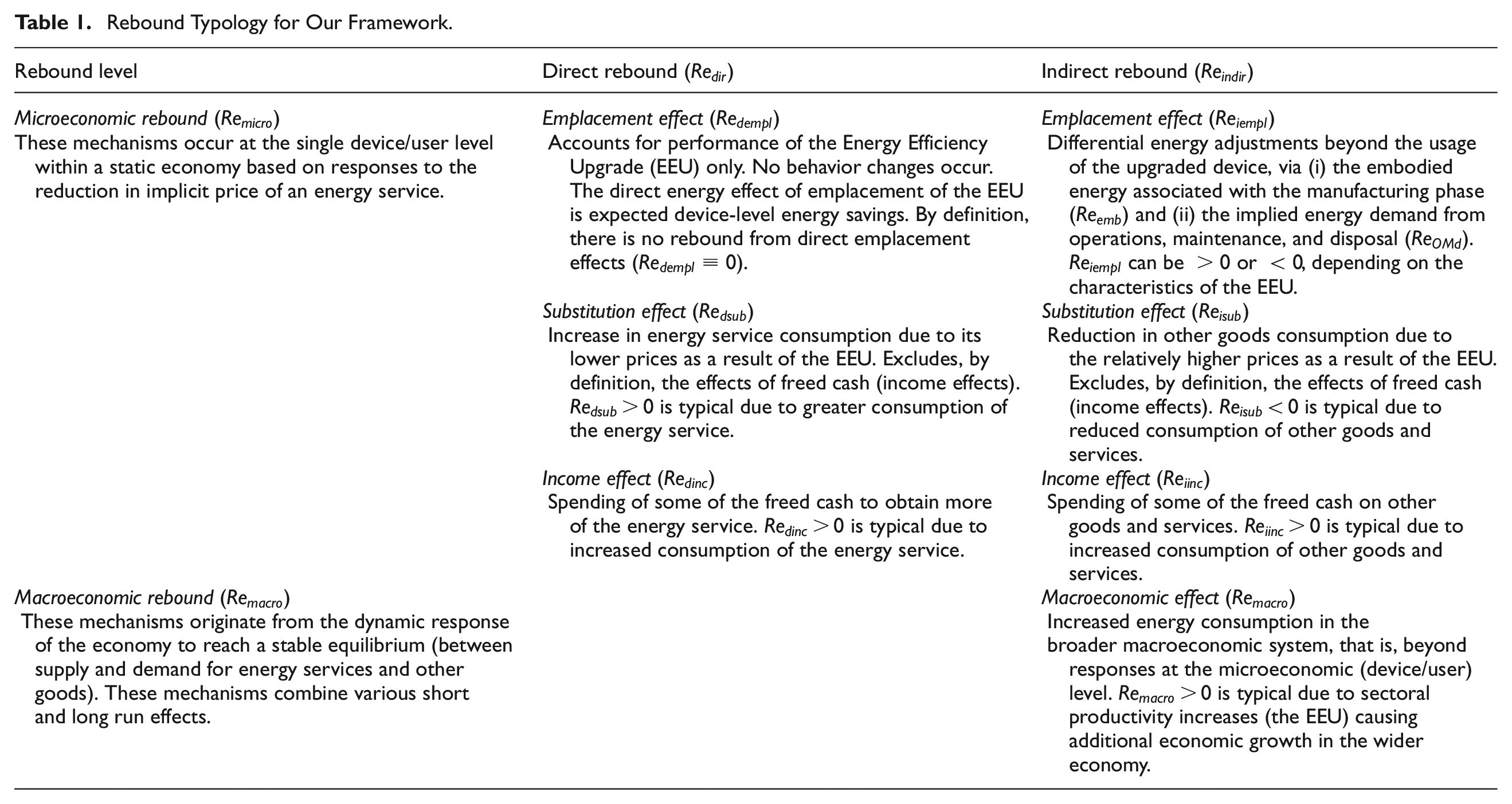
Microeconomic rebound occurs at the level of the single device and its user and in our framework comprises three effects: an emplacement effect, a substitution effect, and an income effect, with direct and indirect partitions for each.
“Emplacement” is a new term we introduce to collect effects associated with installing higher-efficiency devices, including (i) embodied energy of their manufacture (subscript
The direct rebound effect can be partitioned into a direct emplacement effect, a direct substitution effect, and a direct income effect. At the level of the device, all of the direct rebound effects change the consumption of energy by the device whose efficiency has been upgraded, according to a microeconomic behavioral model of the consumer who responds to the cheaper energy service.
Similarly, the indirect rebound effect can be partitioned into an indirect emplacement effect, an indirect substitution effect, and an indirect income effect. All of the indirect effects change the induced energy consumption beyond the upgraded device, again according to a microeconomic behavioral model. We assume a partial equilibrium response to the energy efficiency upgrade (EEU) at the microeconomic level; other prices in the economy (
In contrast, macroeconomic rebound is a broader, economy-wide response to the single device upgrade. Like other authors, we recognize many macroeconomic rebound effects, even if we don’t later distinguish among them. 4 At the macroeconomic level, general equilibrium effects can occur as prices for all goods and services (even energy) may change in response to the EEU. Further treatment of macroeconomic rebound can be found in Section 2.5.4 of this paper (Part I) and in Section 4.1 of Heun et al. (2025). Discussion of an energy price rebound effect can be seen in Section 3.2 below and in Section 4.6 of Heun et al. (2025).
Figure 1 shows rebound effects arranged in the left-to-right order of their discussion in this paper. The left-to-right order does not necessarily represent the progression of rebound effects through time. Rebound symbols are shown above each effect (
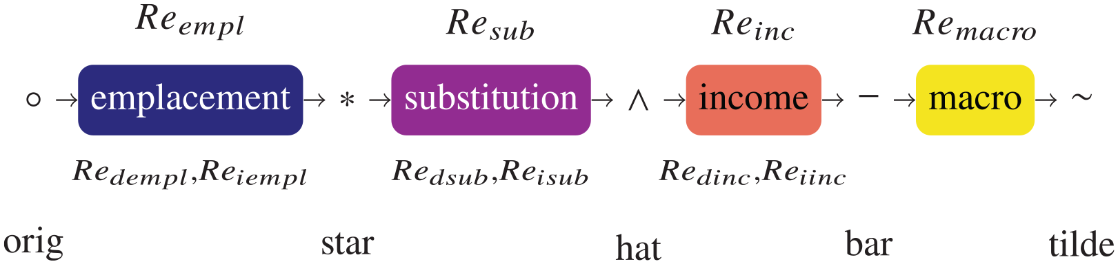
Flowchart of rebound effects and decorations.
2.2. Rebound Relationships
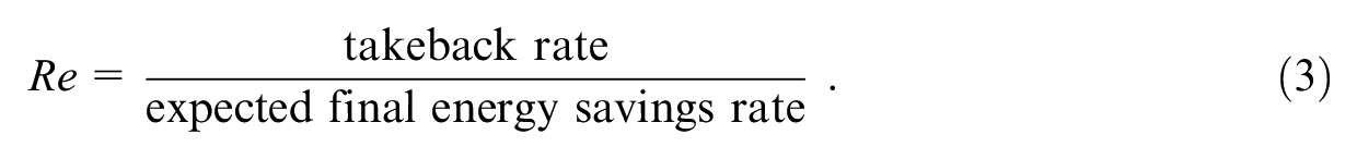
Energy rebound (
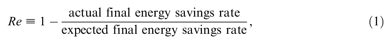
where both actual and expected final energy savings rates are in MJ/yr (megajoules per year) and expected positive. The final energy “takeback” rate is defined as the expected final energy savings rate less the actual final energy savings rate. 6 Rewriting equation (1) with the definition of takeback gives
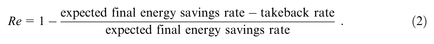
Simplifying gives
We define rebound at the final energy 7 stage of the energy conversion chain, because the final energy stage is the point of energy purchase by the device user. To simplify derivations, we choose not to apply final-to-primary energy multipliers to final energy rates in the numerators and denominators of rebound expressions derived from equations (1) and (3); they divide out anyway. 8 Henceforth, we drop the adjective “final” from the noun “energy,” unless there is reason to indicate a specific stage of the energy conversion chain.
2.3. The Energy Conversion Device and Energy Efficiency Upgrade (EEU)
We assume an energy conversion device (say, a car) that consumes energy (say, gasoline) at a rate
Energy is available at price

where
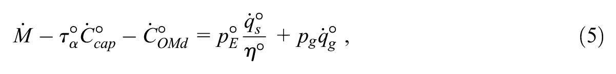
which is the usual discounted budget constraint for the microeconomic consumer after subtracting capital, operations and maintenance, and disposal costs.
Later (Sections 2.5.1–2.5.4), we walk through the four rebound effects (emplacement, substitution, income, and macro), deriving rebound expressions for each, but first we show typical energy and cost relationships (Section 2.4).
2.4. Typical Energy and Cost Relationships
With the rebound notation of Appendix A, four typical relationships emerge. First, the consumption rate of the energy service (


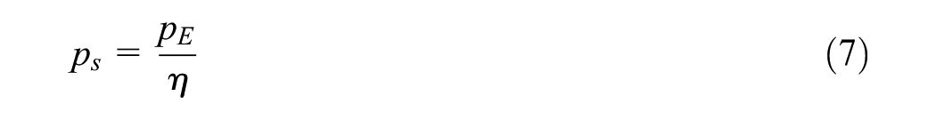
Second, the energy service price (
Third, energy service expenditure rates (


Fourth, indirect energy rates for operations and maintenance (


Note that the indirect energy rate for the disposal effect is obtained from disposal costs that include discounting. (See Appendix B.1 for details on cost discounting.)
2.5. Rebound Effects
The four rebound effects (emplacement, substitution, income, and macro) are discussed in subsections below. In each subsection, we define the effect and show mathematical expressions for rebound (
2.5.1. Emplacement Effect
The emplacement effect accounts for performance changes of the device due to the fact that a higher-efficiency device has been put in service (and will need to be decommissioned at a later date); consumption patterns are assumed unchanged. Behavior adjustments are addressed later, in the substitution and income effects. Any (positive or negative) adjustment in income due to emplacement (measured as net income,
Direct emplacement effect (
(See Appendix B.4.1 for the derivation.)
Because the original and upgraded device are assumed to have equal performance 12 and because behavior changes are not considered in the direct emplacement effect, actual and expected energy savings rates are identical, and there is no takeback. By definition, then, the direct emplacement effect causes no rebound. Thus,

Indirect emplacement effects (
Embodied energy effect (
Consistent with the energy analysis literature, we define embodied energy to be the sum of all energy consumed in the production of the energy conversion device, all the way back to resource extraction.
13
Energy is embodied in the device within manufacturing and distribution supply chains prior to consumer acquisition of the device. We assume no energy is embodied in the device while in service. The EEU causes the embodied energy of the energy conversion device to change from
For simplicity, we spread all embodied energy evenly over the lifetime of the device which gives a constant embodied energy rate (
(See Appendix B.4.2 for details of the derivation.)
Embodied energy rebound (
Operations, maintenance, and disposal effects (
For simplicity, we assume that operations, maintenance, and disposal expenditures imply energy consumption elsewhere in the economy at its overall energy intensity (
(See Appendix B.4.2 for details of the derivation.)
2.5.2. Substitution Effect
Neoclassical economic theory determines consumer behavior through utility maximization. It decomposes price-induced behavior change into (i) substituting energy service consumption for other goods consumption due to the lower post-EEU price of the energy service (the substitution effect) and (ii) spending of the higher real income (the income effect).
14
This section develops mathematical expressions for substitution effect rebound (
After emplacement of the more efficient device (but before the substitution effect), the price of the energy service decreases (
A constant price elasticity (CPE) utility model is often used in the literature (e.g., see Borenstein 2015, 17: footnote 43) for determining post-substitution effect consumption and therefore
Here, we present a constant elasticity of substitution (CES) utility model that allows all of the uncompensated own price elasticity (
The device user’s utility rate (relative to the original condition,
Direct substitution effect rebound (
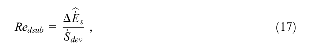
which can be rearranged to
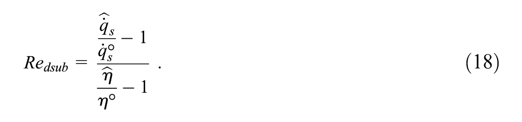
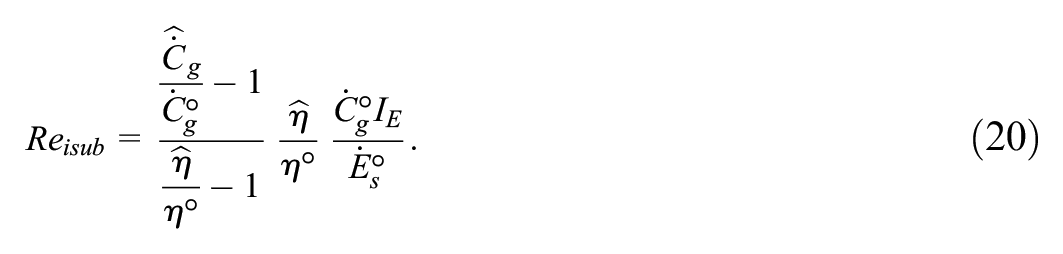
Indirect substitution effect rebound (
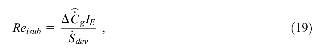
which can be rearranged to
To find the post-substitution effect point (∧), we solve for the location on the indifference curve where its slope is equal to the slope of the post-EEU expenditure line, assuming the CES utility model. 16 The results are
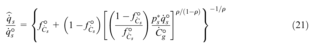
and
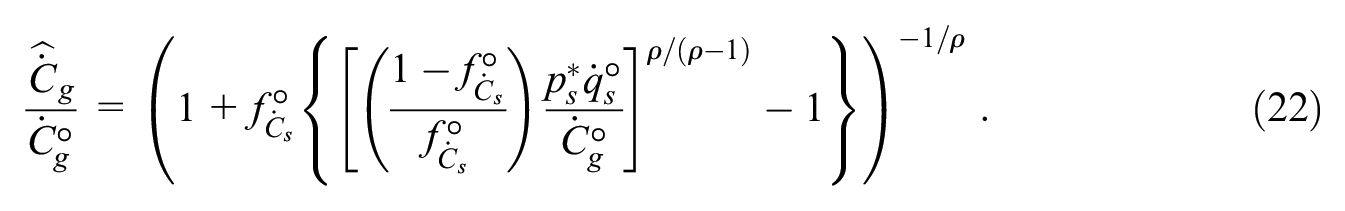
Equation (21) can be substituted directly into equation (18) to obtain an expression for direct substitution rebound (
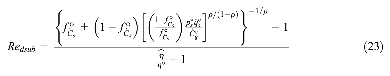
Equation (22) can be substituted directly into equation (20) to obtain an expression for indirect substitution rebound (
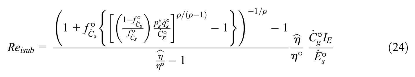
(See Appendix B.4.3 for details of the derivations of equations (18), (20), and (21)–(24).)
2.5.3. Income Effect
The monetary income rate of the device user (
Additional energy demand from the income effect is determined by several constraints. The income effect under utility maximization satisfies the budget constraint, so that net savings are zero after the income effect (
A second constraint is that net savings are spent completely on (i) additional consumption of the energy service (
However, this framework could accommodate non-homothetic preferences for spending across the income effect (turning the income expansion path into a more general curve instead of a line). Demand for certain energy services could satiate as consumers become more affluent, implying income elasticities of the energy service of less than one (Greening, Greene and Difiglio 2000). At the lower bound, the consumer spends all income after the substitution effect on other goods (subscript
We next show expressions for direct and indirect income effect rebound.
Direct income effect (
The ratio of rates of energy service consumed across the income effect is given by
Under the CES utility model, homotheticity means that
Effective income (
For the purposes of the income effect, effective income (equation (26)) adjusts original income (
Direct income rebound is defined as

(See Table B.5.) After substitution, rearranging, and canceling of terms (Appendix B.4.4), the expression for direct income rebound under the CES utility model is
If there are no net savings after the substitution effect (
Under a non-homothetic utility model, the bounding condition is satiated consumption of the energy service such that as the device owner becomes richer, none of the net income (
Indirect income effect (
The ratio of rates of other goods consumed across the income effect is given by
Under the assumption that prices of other goods are exogenous (see Appendix E), the ratio of rates of other goods consumption (
Homotheticity means that
After substitution, rearranging, and canceling of terms, the expression for indirect income rebound under the CES utility model is
(See Appendix B.4.4 for details of the derivation of direct and indirect income effect rebound.)
Under the bounding satiated utility model, all net income (
2.5.4. Macro Effect
The previous rebound effects (emplacement effect, substitution effect, and income effect) occur at the microeconomic level. However, changes at the microeconomic level can have important impacts at the macroeconomic or economy-wide level.
It is one of the basic tenets of economics that productivity gains have been the main long-run driver of economic growth in the last couple of centuries (Marx 1867; Smith 1776; Solow 1957). Interest in the impact of individual sectors on the whole economy reaches arguably even farther back (Quesnay 1759) and continues to the present (Leontief 1986). Recent work revived interest in firm- and sector-specific shocks on aggregate output and demonstrates that due to interlinkages between firms and sectors, productivity shocks in a firm or sector can have larger macroeconomic consequences than the original shock (Acemoglu et al. 2012; Baqaee and Farhi 2019; Gabaix 2011). Foerster et al. (2022) estimate that 3/4 of long-run U.S. growth since 1950 can be attributed to sector-specific (as opposed to aggregate) trend factors. Because the EEU represents a positive, sector-specific productivity shock, the same principles apply. These kinds of rebounds can be captured by a general equilibrium model (Stern 2020), but we propose a simple rule for incorporating this macroeconomic effect of productivity growth into our partial equilibrium framework.
Before establishing a formalism for
Borenstein also addressed these macro effects from consumer behavior noting that “income effect rebound will be larger economy-wide than would be inferred from evaluating only the direct income gain from the end user’s transaction” (Borenstein 2015, 11) and likened it to a macroeconomic multiplier.
21
The sectoral growth shock literature also uses multipliers to conceptualize the impacts of sectoral productivity shocks on aggregate output (Buera and Trachter 2024; Foerster et al. 2022). Using multipliers has the advantage that they can be directly linked to the income effect (minus compensating variation) and its consequence for macroeconomic rebound. Borenstein also notes that scaling from net savings (
We operationalize the macro rebound multiplier idea by noting that higher productivity makes the device cheaper to operate (and possibly purchase), which allows consumers to purchase a larger bundle of goods and services. If the overall expansion of the economy is a multiple of the direct increase in productivity expressed as productivity gains in other sectors, then the macro effect can simply be represented as a multiple of the (indirect) emplacement effect at the post-emplacement stage (*) of Figure 1, a multiplier that we represent by a macro factor (
The macro factor (
We assume as a first approximation (following Antal and van den Bergh 2014; Borenstein 2015) that macro effect responding implies energy consumption according to the average energy intensity of the economy (

(See Table B.6.) After some algebra (Appendix B.4.5), we arrive at an expression for macro effect rebound:

Another macroeconomic rebound could arise from the energy price, which could fall due to lower demand (Borenstein 2015; Gillingham, Rapson and Wagner 2016). The size of the energy price effect depends on the size of the energy savings from the EEU relative to the energy demand in the economy. Therefore, calculating the energy price effect requires additional assumptions about how many households adopt the new device, which we consider to be outside the scope of our core framework. However, we show how it could be incorporated by adding an assumption about EEU adoption shares and a model of the energy market to derive a rebound expression for the energy price effect in Section 3.2 and Appendix F.
2.6. Rebound Sum
The sum of all rebound emerges from the four rebound effects (emplacement effect, substitution effect, income effect, and macro effect). Macro effect rebound (
3. Discussion
3.1. Comparison to Other Rebound Frameworks
We developed above a rebound framework for consumers. We note that many of its components are similar to those for a producer-sided framework due to symmetries between neoclassical microeconomic producer and consumer theory. Ours is a partial equilibrium framework at the microeconomic level that provides a detailed assessment of individual EEUs with tractable, easy-to-understand mathematics. Partial equilibrium frameworks are easier to understand, in part, because they constrain price variation to the energy service only; all other prices remain constant (at least at the microeconomic level). 23 In our framework, general equilibrium effects and other dynamic effects at the macroeconomic level are captured by a simplified, one-dimensional rebound effect discussed in Section 2.5.4.
We are not the first to develop a rebound analysis framework, so it is worthwhile to compare our framework to others for key features: analysis of all rebound effects; analysis of energy, expenditure, and consumption aspects of rebound; level of detail in the consumer preference model; allowance for non-marginal energy efficiency changes; and empirical application. When all of the above characteristics are present, a fuller picture of rebound can emerge. 24 Table 2 shows our assessment of selected previous partial equilibrium frameworks (in columns) relative to the characteristics discussed above (in rows).
Comparison Among Relevant Rebound Analysis Frameworks.
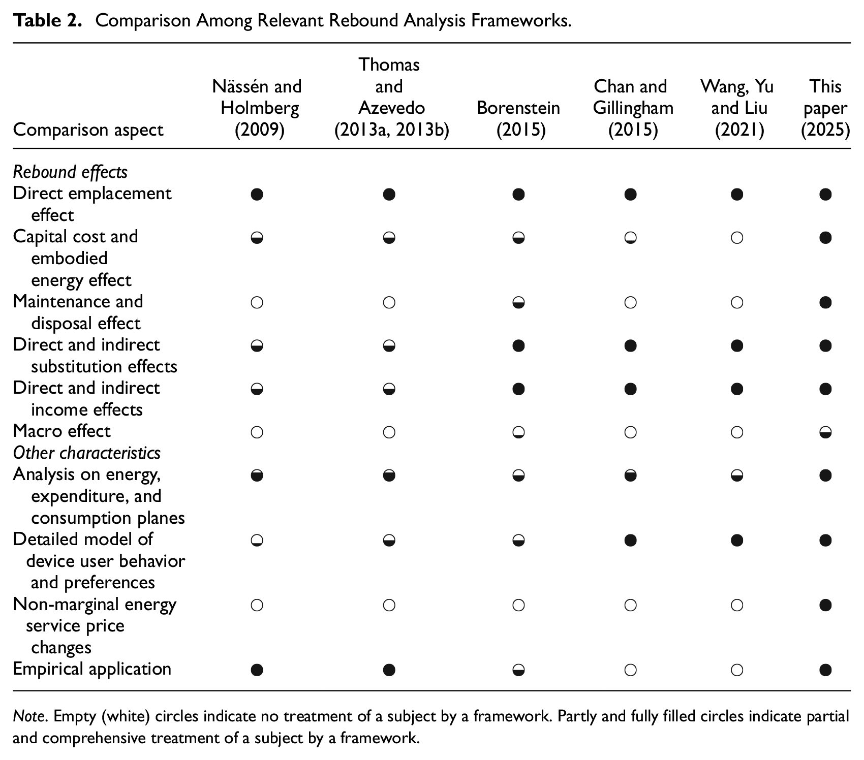

Note. Empty (white) circles indicate no treatment of a subject by a framework. Partly and fully filled circles indicate partial and comprehensive treatment of a subject by a framework.
Because all frameworks evaluate the expected decrease in direct energy consumption from the EEU, the “Direct emplacement effect” row contains • in all columns. Three early papers (Nässén and Holmberg 2009; Thomas and Azevedo 2013a, 2013b) estimate rebound quantitatively, earning high marks (•) in the “Empirical application” row. Both Nässén and Holmberg and Thomas and Azevedo motivate their frameworks at least partially with microeconomic theory (consumer preferences and substitution and income effects) but use simple linear demand functions in their empirical analyses. Thus, the connection between economic theory and empirics is tenuous, leading to intermediate ratings (◒ or less) in the “substitution effects,”“income effects,” and “Detailed model of consumer preferences” rows. More recently, Chan and Gillingham (2015) and Wang, Yu and Liu (2021) anchor the rebound effect firmly in consumer theory, earning high ratings (•) in the “substitution effects,”“income effects,” and “Detailed model of consumer preferences” rows. They extend their frameworks to advanced topics that our framework does not presently incorporate, such as multiple fuels, energy services, and nested utility functions with intermediate inputs. However, neither Chan and Gillingham nor Wang et al. provide empirical applications, earning ○ in the last row of Table 2. In the middle of the table (and between the other studies in time), the framework by Borenstein (2015) touches on nearly all important characteristics. However, the Borenstein framework cannot separate substitution and income effects cleanly in empirical analysis, reverting to partial analyses of both, leading to a ◒ rating in the “Detailed model of consumer preferences” and “Empirical application” rows.
No previous framework engages fully with either the differential financial effects or the differential energetic effects of the upfront purchase of the upgraded device, leading to low ratings across all previous frameworks in the “Capital cost and embodied energy effect” row. In fact, except for Nässén and Holmberg (2009), no framework engages with capital costs, although all note its importance. (Nässén and Holmberg note that capital costs and embodied energy can have very strong effects on rebound.) Thomas and Azevedo (2013a, 2013b) provide the only framework that traces embodied energy effects of every consumer good using input-output methods, but they do not analyze embodied energy of the upgraded device. Borenstein (2015) notes the embodied energy of the upgraded device and the embodied energy of other goods but does not integrate embodied energy or financing costs into the framework for empirical analysis. Borenstein is, however, the only author to treat the financial side of embodied energy or maintenance and disposal effects. Borenstein (2015) postulates the macro effect, but does not operationalize the link between micro and macro levels, earning ◒ in the “Macro effect” row. No other framework even discusses the link between macro and micro rebound effects, leading to ° in the “Macro effect” row for all previous frameworks (apart from Borenstein 2015). Our framework operationalizes the link between micro and macro levels, via the macro factor (
Table 2 shows that previous frameworks contain many key pieces, providing starting points from which to develop our rebound analysis framework. A left-to-right reading of the table demonstrates that previous frameworks start from microeconomic consumer theory and move towards more rigorous theoretical treatment over time, with recent frameworks making important advanced theoretical contributions at the expense of empirical applicability. In the end, no previous rebound analysis framework combines all rebound effects across energy, expenditure, and consumption aspects with a detailed model of consumer preferences, non-marginal energy service price changes, and empirical applicability for the simplest case (understandable across disciplines) of a single fuel and a single energy service. In particular, assessing the rebound implications of differential capital costs, non-marginal price changes, and the macro effect required conceptual development as in Section 2.5.4 and Appendix B.4.5. (Development of empirical applications is left for Heun et al. (2025).) This paper addresses most of the gaps in Table 2; hence we fill the “This paper (2025)” column with filled circles (•) in nearly all rows. By so doing, we help advance clarity in the field of energy rebound.
3.2. Notes on an Energy Price Rebound Effect
The income effect (Section 2.5.3) captures the energy and rebound implications of expanding real income at the level of the upgraded device. The partial equilibrium framework described herein enables calculation of income effect rebound (
But there are other effects at work beyond the device level and outside the boundaries of a partial equilibrium analysis. One of those effects is an energy price effect. This section (and Appendix F) shows that our partial equilibrium framework can be extended to obtain an initial estimate of the rebound implications of an energy price effect (
The energy price effect can lead to rebound when EEUs are applied to energy conversion devices at a scale that is substantial relative to the economy-wide use of energy. Examples of conditions under which the energy price effect could be significant include replacing all cars in the economy by hybrids and replacing all domestic electric lamps in the economy by LEDs, to use the examples from Heun et al. (2025). With reduced energy demand throughout the economy, an energy price reduction can be expected (
A complete analysis of the price effect would amount to introducing a full model of the energy market and involve solving a system of simultaneous equations for the new economy-wide energy demand, the new energy price, and a new consumption bundle. But in this instance, as we desire a simple estimate of energy price rebound, we conservatively assume the device owner spends the additional freed cash (the result of the lower energy price) exclusively on other goods, with energy implications at the energy intensity of the economy (
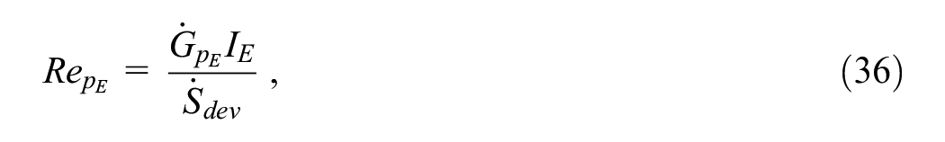
where
4. Conclusions
In this paper (Part I), we developed foundations of a rigorous analytical framework that includes all rebound effects across energy, expenditure, and consumption aspects with a detailed model of consumer preferences and non-marginal energy service price changes in an operational manner linking micro and macro effects for the simplest case of a single fuel and a single energy service. Furthermore, we presented approaches for exploring consumer satiation of energy service demand and for analyzing the effect of reduced energy demand on energy price to create energy price rebound. With careful explication of rebound effects and clear derivation of rebound expressions, we help advance the analytical foundations for empirical analyses and facilitate interdisciplinary understanding of rebound phenomena toward the goal of enhancing clarity in the field of energy rebound and enabling more robust rebound calculations for sound energy and climate policy.
Future work could be pursued in several areas. (i) Other utility models (besides the CES utility model, but not a Cobb-Douglas utility model) could be explored for the substitution effect. (ii) Although this is a consumer-sided framework, we demonstrated that it could be extended to effects affecting producers such as the energy price rebound effect. Further work could explore additional extensions to other producer-sided energy rebound effects. Moreover, a neoclassical producer framework, in analogy to the consumer framework, could be derived due to the substantial symmetry between neoclassical consumer and producer models (Fine 2016; Varian 1992). (iii) This framework could be extended to include some of the advanced topics in Chan and Gillingham (2015) and Wang, Yu and Liu (2021), such as multiple fuels or energy services, more than one other consumption good, and nested utility functions with intermediate inputs. (iv) This framework could be extended to include fuel-switching EEUs, wherein the upgraded device uses a different fuel from the original device. (v) The greenhouse gas emissions implications of energy rebound could be evaluated using this framework, provided that the primary energy associated with final energy purchases were available. Borenstein (2015) went some way to analyzing emissions and could provide a starting point for such work. The capability to analyze fuel-switching EEUs (discussed in the previous item) will be important for analyzing the greenhouse gas emissions implications of many EEUs that involve electrification, such as the transition to all-electric vehicles and the conversion of natural gas and oil furnaces to heat pumps for home heating.
In Heun et al. (2025), we further help advance clarity in rebound analysis in three ways. First, we develop a way to visualize the energy, expenditure, and consumption aspects of rebound effects. Second, we apply the framework to two EEUs: an upgraded car and an upgraded electric lamp. Finally, we provide results of rebound calculations for the two examples.
Footnotes
Appendices
Acknowledgements
The authors benefited from discussions with Daniele Girardi (University of Massachusetts Amherst) and Christopher Blackburn (Bureau of Economic Analysis). The authors are grateful for comments from internal reviewers Becky Haney and Jeremy Van Antwerp (Calvin University); Nathan Chan (University of Massachusetts Amherst); and Zeke Marshall (University of Leeds). The authors appreciate the many constructive comments on a working paper version of this article from Jeroen C. J. M. van den Bergh (Vrije Universiteit Amsterdam), Harry Saunders (Carnegie Institution for Science), and David Stern (Australian National University). Finally, the authors thank the students of MKH’s Fall 2019 Thermal Systems Design course (ENGR333) at Calvin University who studied energy rebound for many energy conversion devices using an early version of this framework.
The findings, interpretations, and conclusions expressed in this paper are entirely those of the authors. They do not necessarily represent the views of the International Bank for Reconstruction and Development/World Bank and its affiliated organizations, or those of the Executive Directors of the World Bank or the governments they represent.
Author Contributions
Matthew Kuperus Heun: Conceptualization, Methodology, Validation, Investigation, Resources, Writing—Original Draft, Writing—Review & Editing, Supervision, Project Administration. Gregor Semieniuk: Conceptualization, Methodology, Investigation, Resources, Writing—Original Draft, Writing—Review & Editing. Paul E. Brockway: Methodology, Validation, Resources, Writing—Review & Editing, Funding Acquisition.
Declaration of Conflicting Interests
The author(s) declared no potential conflicts of interest with respect to the research, authorship, and/or publication of this article.
Funding
The author(s) disclosed receipt of the following financial support for the research, authorship, and/or publication of this article: Paul Brockway’s time was funded by the UK Research and Innovation (UKRI) Council, supported under EPSRC Fellowship award EP/R024251/1, and latterly by Leverhulme Trust Research Project Grant RPG-2024-357.
1
We prefer the term “energy analysts” over “engineers,” because “energy analysts” better describes the group of people engaged in “energy analysis.” For this paper, we define “energy analysis” to be the study of energy transformations from stocks to flows and wastes along society’s energy conversion chain for the purpose of generating energy services, economic activity, and human well-being.
2
Indeed, this is why the authors for these papers come from the disciplines of energy analysis (MKH, PEB) and economics (GS).
3
This objective may mean that some aspects of the development of the framework will seem obvious to energy analysts while other aspects will seem obvious to economists.
4
For example, Sorrell (2009) sets out five macroeconomic rebound effects: embodied energy effects, responding effects, output effects, energy market effects, and composition effects. (We place the embodied energy effect at the microeconomic level.) Santarius (2016) and Lange et al. (2021) introduce meso (i.e., sectoral) level rebound between the micro and macro levels. ![]() distinguishes 14 types of rebound, providing, perhaps, the greatest complexity.
distinguishes 14 types of rebound, providing, perhaps, the greatest complexity.
5
Note that the vocabulary and mathematical notation for rebound effects is important; ![]() and Appendix A provide guides to elements used throughout this paper, including symbols, Greek letters, abbreviations, decorations, and subscripts. The notational elements can be mixed to provide a rich and expressive symbolic “language” for energy rebound. As the goal of this paper is to bridge disciplines, the nomenclature will necessarily have unfamiliar elements to each discipline involved.
and Appendix A provide guides to elements used throughout this paper, including symbols, Greek letters, abbreviations, decorations, and subscripts. The notational elements can be mixed to provide a rich and expressive symbolic “language” for energy rebound. As the goal of this paper is to bridge disciplines, the nomenclature will necessarily have unfamiliar elements to each discipline involved.
6
Note that the takeback rate can be negative, indicating that the actual final energy savings rate is greater than the expected final energy savings rate, a condition called hyperconservation.
7
Conventionally, stages of the energy conversion chain are primary energy (e.g., coal, oil, natural gas, wind, and solar), final energy (e.g., electricity and refined petroleum), useful energy (e.g., heat, light, and mechanical drive), and energy services (e.g., transport, illumination, and space heating). See ![]() for an introduction to societal energy and exergy accounting.
for an introduction to societal energy and exergy accounting.
8
9
We discount money because interest changes the available amount of money over time. In contrast, we do not discount energy, because there is no temporal variation in the ability of energy to effect changes (via heat or work) in the physical world. We thank an anonymous reviewer for the insight that, in principle, the carbon content of energy could also be discounted if one assumes that near term emissions are worse than later emissions.
10
Relaxing the exogenous energy price assumption would require a general equilibrium model that is beyond the scope of this paper. However, see Section 3.2 where we discuss an energy price rebound effect as an extension of this framework.
11
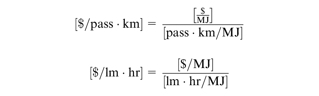
Note that “pass” is short for “passenger,” and “lm” is the SI notation for the lumen, a unit of lighting energy rate.
12
Of course, it is often the case that the original and upgraded devices have small performance differences. For example, a high-efficiency LED lamp may have slightly greater or slightly lesser lumen output than the incandescent lamp it replaces. For the purpose of explicating this framework, we assume that the performance of the upgraded device can be matched closely enough to the performance of the original device such that the differences are immaterial to the user.
13
We take an energy approach here, consistent with the literature on energy rebound. One could use an alternative quantification of energy, such as exergy, the work potential of energy (Sciubba and Wall 2007) or emergy, the solar content of energy (![]() ).
).
14
For the original development of the decomposition see Slutsky (1915) and Allen (1936). For a modern introduction see ![]() .
.
15
Alternative assumptions on behavior would arise from, for example, adopting a behavioral economic framework (Dorner 2019; Dütschke et al. 2018) or an informational entropy-constrained economic framework (![]() ).
).
16
Other utility models could be used; however, the Cobb-Douglas utility model is inappropriate for this framework, because it assumes that the sum of substitution and income rebound is 100% always. Regardless of the utility model, expressions for ![]() ), respectively.
), respectively.
17
18
Zero net savings (
19
To appreciate the difference between production for the market and production for the household, consider the example of increased fuel efficiency. In one case, the household upgrades its own car and takes more trips (direct rebound), without effect on GDP. In the other case, the household buys the energy service (transport) directly from a taxi company that upgrades its cars. Here, the taxi company lowers the price but gains more customers, leading immediately to growth in inflation-adjusted (i.e., real) GDP, as more driving services are produced. Yet, the physical change of more car trips is the same in both cases.
20
Nevertheless, as long as the energy efficiency improvement (in this example, an upgraded car) is the only technological progress in the economy, further output growth may be constrained to the extent that the other inputs into production remain constrained at their original levels and substituting energy for the other inputs to production is limited by the prevailing technology.
21
It is important to distinguish this multiplier from an autonomous expansion of expenditure, a demand-side shock, in an otherwise unchanged economy, that is, the Keynesian multiplier (Kahn 1931; Keynes 1936), that risks crowding out other economic activity (Gillingham, Rapson and Wagner 2016). Our energy productivity improvement is a supply-side shock. After the EEU, it takes less energy (and therefore less energy cost) to generate the same economic activity, because energy efficiency has improved, so the concept of crowding-out as defined by macroeconomics does not apply.
22
The macro factor (
23
General equilibrium frameworks provide detail and precision on economy-wide price adjustments, but they give up specificity about individual device upgrades, make assumptions during calibration, and lose simplicity of exposition.
24
25
In principle, calculated arc elasticities could describe the relationship between price and quantity changes for any EEU by representing the percentage price and quantity changes between any two known consumption bundles (![]() ). However, we do not know the new consumption bundle and instead determine it with the CES utility function whose price elasticities vary along the indifference curve.
). However, we do not know the new consumption bundle and instead determine it with the CES utility function whose price elasticities vary along the indifference curve.
26
27
For