Sage Journals: Discover world-class research

Abstract

After the 2008 World Crisis, there is a view that the economic recovery has not been adequate. In this context, the debate on hysteresis and especially investment hysteresis has increased in the last decade. The aim of this study is to analyze the investment hysteresis and the basic dynamics of hysteresis in the Turkish economy. Structural break tests are used to identify hysteresis. Traditional and asymmetric causality tests are used to identify the fundamental dynamics of hysteresis. Investment, GDP, interest rate, and productivity variables are used to analyze investment hysteresis. Structural break tests were applied to the variables, while conventional and asymmetric causality tests were applied between investments and their determinants. Structural break tests prove the existence of hysteresis. According to the Granger causality test, there is no causality from interest rates, GDP and productivity to investments. The fact that interest rates have no effect on investments proves hysteresis. According to the asymmetric causality test, there is no relationship between interest rates and investments. There is an inverse relationship between GDP and investments. There is an asymmetric relationship between productivity and investments. The fact that productivity shocks cause asymmetric effects on investments makes productivity shocks the main dynamic of hysteresis. In addition, there is considerable evidence that the strong hysteresis and high uncertainty of TFP exacerbate investment hysteresis. Therefore, productivity shocks should be taken into account in policymaking for hysteresis.

Keywords

investment hysteresis structural breaks asymmetric causality E12 E22 L10

Introduction

Although the determinants of investments have always been the subject of discussion in mainstream economics, they have become even more intense today. The importance of investment stems from the fact that they are the main dynamics of the supply side in economic activity. The harmony between economic growth and investments, regardless of developed and developing economies, proves this situation. However, the fact that investments have not been able to recover after an economic shock and at the same time, are not able to show the expected performance despite the necessary conditions for their return to old levels has brought the phenomenon of hysteresis in investments to the agenda.

Due to the insufficient capital formation in the Turkish economy, the financing of investments also becomes important. Regardless of the distinction between public and private investments, there is a causality relationship between investment and growth. Therefore, the absolute growth rate of investments is a determinant of economic growth (Khan & Reinhart, 1990). Based on this information, the insufficient level of capital formation in the Turkish economy will not cause a growth problem above its potential. In this context, the absence of an efficiency problem in terms of the marginal product of capital directs the motivation of empirical studies toward the size of investments. On the other hand, the existence of strong empirical evidence that financial development affects growth through the investment channel in the Turkish economy makes investments extremely important for a sustainable growth performance (Xu, 2000). The fact that investments are a transmission mechanism in the reflection of demand growth to supply-side growth as a result of financial development makes investments vitally important. As a result, the hysteresis phenomenon, which creates efficiency problems in investments, constitutes a major obstacle to growth and development. Therefore, the main objective of this study is to identify hysteresis in investments, to identify the dynamics that cause hysteresis in investments and to propose effective policies to solve hysteresis.

Cerra et al. (2022) argue that traditional approaches analyze business cycles separately from economic growth. However, the hysteresis phenomenon argues that current imbalances in the economy should be associated with past shocks. Furceri et al. (2021) argue that recessions cause declines in output and production inputs as well as Total Factor Productivity (TFP) which declines over 3–5 years, while Cerqueira and Martins (2009) argue that low productivity in investment limits output. The standard production function attributes output hysteresis to declines in TFP, employment, and capital. Adler et al. (2017) show that TFP and investment hysteresis are the main dynamics in the long-run spread of output losses in economic crises in low-income countries. Jordà et al. (2020) also show that TFP and capital stock exhibit hysteresis behavior, while no hysteresis is observed in the labor force, proving that TFP and investments are determinants of output hysteresis.

Tervala (2021) finds that output hysteresis increases the welfare cost of recessions. Therefore, stronger stabilization policies are needed in policymaking. In addition, Ball (2015) argues that an expansionary policy (high-pressure economy) with high growth potential should be implemented. Recessions have a lasting impact on TFP and potential output. However, it is concluded that public spending is the most effective policy tool in economic recovery (Tervala and Watson, 2022). As a matter of fact, not implementing active expansionary policies in hysteresis will cause hysteresis to spread over a longer period. On the other hand, Benhabib and Spiegel (2000) argue that financial development is based on TFP and investments. Based on the incentive effect of financial development on investment, the investment hysteresis not only determines output but also determines the investment hysteresis as its dynamic. As a result, based on the cyclical process between investment and output, the solution of investment hysteresis will be an effective policy tool for output hysteresis. This reveals that investment hysteresis is crucial for output.

In the theoretical and empirical literature, there is a debate on the determinants of investments. In this context, according to the neoclassical investment theory, the marginal return on investment is equated with the interest rate, in other words, the view that investments are a function of the interest rate is accepted. In the Keynesian view, the marginal productivity of capital and the expected return on investments determine the volume of investment. On the New Keynesian basis, Hicks synthesized these two views and argued that the Keynesian view would prevail in the short run and the Neoclassical view in the long run (Gordon, 1992; Lopez & Mott, 1999). The views of Post Keynesians are closer to the Keynesian view. Poitras (2002) argues that Post Keynesians, synthesized with Keynes and Kaleckigian views, basically argue that investment is determined by the marginal efficiency of capital and the interest rate in the long run. As a matter of fact, the level of profit is the determining factor in investment demand. Arestis (1996), on the other hand, the acceptance of the profit rate as the financing of investments causes profits to have a dual function in the Post Keynesian framework. This process shows that the level of profit is a determinant of both investment demand and investment financing. As a result, according to investment theories, there is no consensus on the determinants of investments. The existence of uncertainty in the determinants of investments and investments provides evidence for this situation. Hu et al. (2022) argue that increased uncertainty reduces the effectiveness of economic policies and Liang et al. (2020) argue that it also reduces the efficiency of investments by reducing the effectiveness of investment decisions. Studies on the relationship between investment and output in terms of uncertainty (Hong et al., 2022; Baker et al., 2016) indicate that uncertainty leads to an increase in investment costs and reduces investment and output. Hysteresis can be detected from the behavior of an economic variable. At the same time, hysteresis can also be detected from the response of an economic variable to its determinants. Therefore, the course of investments and the response to the determinants of investments are important in detecting hysteresis. Based on this information, the motivation of the study is directed towards hysteresis analysis through the determinants of investments and their relationship with the determinants of investments in addition to the structural break tests commonly used in the empirical literature.

In terms of the Turkish economy, the analysis variables are constructed by taking into account the theoretical foundations and empirical literature. Fixed capital formation, which includes private and public sector investments, is determined as the investment variable. Uçan and Öztürk (2011) argue that since financial development has a positive effect on investments in the Turkish economy, the interest rate in terms of ease of finance is a determinant variable for investments. On the other hand, the positive relationship between GDP and investments provides a basis for the theory that investments are a function of income, while Levine and Renelt (1992) empirically prove this by finding a strong long-run relationship between investments and economic growth, which puts economic growth in an important position in detecting hysteresis effects. Jorgenson (1963) In neoclassical theory, Irving Fisher emphasized the positive effect of productivity on investment performance. Based on this theoretical and empirical background, investments (fixed capital formation), productivity (the ratio of investments to total industrial production), GDP, and interest rate (average cost of funding) are set as the variables of analysis. Focusing not only on the investment behavior but also on the relationship between the determinants of investments and the determinants of investments in the detection of hysteresis allows us to determine which investment theory is valid for investments, to identify the basic dynamics of hysteresis and, accordingly, to determine the optimum policy for solving hysteresis. As a matter of fact, designing the empirical approach in this way constitutes the original value of the study.

The most widely used method for hysteresis in the empirical literature is structural break analysis. Findings from structural break analyses prove the validity of hysteresis in investments by pointing to the existence of a structural break in investments. However, the main objective of the study is to identify the dynamics that cause hysteresis beyond the detection of hysteresis, which leads to the causality relationship between investments and the determinants of investments. In this context, the absence of a traditional (Granger) causality relationship between investments and their theoretical determinants necessitated the analysis of asymmetric relationships, which is the determinant structural feature of hysteresis. In the empirical literature on hysteresis effects, the analysis of asymmetric relationships has a large place and the presence of asymmetric relationships is interpreted as hysteresis. According to the results of the asymmetric causality test, there is no asymmetric relationship between interest rates and GDP and investments, whereas there is an asymmetric causality relationship between productivity and investments. These findings prove the validity of hysteresis in investments. At the same time, it is concluded that the main dynamic of hysteresis is productivity shocks. As a measure of uncertainty, the Ornstein–Uhlenbeck/Vasicek Model long-run variance results provide important evidence for hysteresis. The fact that investments have higher uncertainty than GDP proves the uncertainty in investments. Moreover, the fact that productivity has the highest uncertainty as the main dynamic causing hysteresis in investments points to a structure that deepens hysteresis.

Finally, the study will be concluded with the conclusion part by giving place to the empirical literature in the second part, the theoretical framework in the third part, and the method and empirical findings in the fourth part.

Theoretical Framework

There is a debate on the determinants of investments in terms of investment theories. Therefore, to effectively analyze investment behavior in hysteresis analysis, it will increase the effectiveness of the study to investigate investment theories, the determinants of investments on the theoretical basis and the approaches used in the empirical literature.

Clark (1979) argues that interest in the behavior of investments has increased since the early 1970s with the relative slowdown in investments despite growth performance. In this context, the determinants of investment were first examined to explain investment behavior. As determinants of investment, investments are a decreasing function of the cost of investment, investments are determined by firm output in the short run and interest rates in the long run. Therefore, the main variables determining investment behavior are cost, output (firm income) and interest rates. While these variables as determinants of investments are based on a static analysis, it is also possible to analyze them in a dynamic process as the Steigum (1983) flexible accelerator model of investments. Instead of determining a certain optimum point in long-term investments, firms determine their investment strategy according to decreasing cost conditions based on cost changes, changes in profit rates and interest rate changes. As a result, static and dynamic analysis processes in terms of determining investments have reached a consensus in terms of cost, income and interest rate variables.

Although hysteresis effects in investments are defined with different approaches in the literature, two important features come to the fore. When there is a shock affecting investment, it deviates from the general equilibrium and stabilizes in the new trend (Piscitelli et al., 2000). The other approach is the behavior of investments involving high fixed costs, known as irreversible investments, which explains the hysteresis effects in terms of sunk costs (Carruth and Henley, 2000). It is the delay of investment decisions due to sunk costs after negative shocks in the economy. Beyond delayed investments, exit decisions are also delayed due to high sunk costs. At the same time, the increase in risk and uncertainty reduces the expected return on investment. This process weakens the relationship between investments and their determinants. In this context, the delayed entry and exit from the market, the persistence of investments by not returning to their previous level after a negative shock and the decrease in their sensitivity to the determinants of investments are interpreted as hysteresis.

When different investment theory approaches are examined, it is seen that the theoretical framework is determined according to cost, income and interest variables in determining investment behavior. Modigliani and Miller (1958), who explain the cost approach based on the cost of capital, state that firm cost is determined by aggregating borrowing costs, return on equity, return on bonds and return on equity. Firms determine their investments by taking into account the aggregated cost, net profit and market value of the firm. Isham and Kaufmann (1999) However, the World Bank emphasizes that investment behavior is significantly affected by the increasingly competitive environment due to financial liberalization and puts efficiency at the center of investment behavior. On the basis that the marginal productivity of investments determines investment behavior, investments will increase in economies with high growth potential until the point of diminishing return conditions. While these conditions better explain short-term investment behavior, in the long run, the expected return on investments better explains investment behavior.

Long-run investment behavior is shaped according to the expected return on investments (Fisher, 2000). The firm determines its investment decision between the future and the present according to the total cost conditions. When the net present value of the investment, known as the alternative cost of not investing, is equal to the current period return, the firm is expected to be inactive in its investment behavior. It arises from the fact that the behavior of being inactive in terms of investment decision can have a prediction about the expected return by waiting. Schmitt-Grohe et al. (2012), intertemporal investment behavior is determined according to the net present value theory. Notation variables;

Y₁: firm’s current period income, Y₂: firm’s future income, I₁: firm’s current investment, I₂: firm’s future investment, r₀: current period interest rate, r₁: current period interest rate, (1 + r₀) B^Y: firm’s investment The expected return of the investment between periods is presented in equation (1), while it is defined as the initial value of the income

Y_{1} + \frac{Y_{2}}{1 + r_{1}} = I_{1} + \frac{I_{2}}{1 + r_{1}} + (1 + r_{0}) B^{Y}

(1)

In other words, equivalence is defined as the firm’s budget constraint for intertemporal investments. According to this notation, the firm allocates its investments between the present and the future. If the expected future return on investments (net present value) is higher than the current period, no investment will be made. On the other hand, if the return on investments in the current period is higher than the net present value, the current period is chosen for investment preference. Since changes in foreign interest rates also determine relative interest rates in open economies, world interest rate shocks may also affect this process. If domestic interest rates are relatively high, investment in the current period tends to be reduced and postponed to future periods.

The Feldstein-Horioka Paradox, which stands out as an important structural issue in developing countries, emphasizes GDP growth instead of savings as the determinant of investments. Kaygısız et al. (2016), Ethem et al. (2012), and Altıntaş and Taban (2011) are the prominent empirical studies that provide evidence for this situation. Kinnon (1973) and Shaw (1973), who evaluated the impact of the financial liberalization process on investments through the growth performance of countries, reached the empirical finding that the effect of financing volume on investments was higher than the effect of financing costs. Akkina and Celebi (2002), who tested the value of financing on investments for Turkey, observed that the value added of investment expenditures in terms of growth is higher than other expenditure items, but that it causes some crowding out effect during financial liberalization. Theoretically, since revenues constitute the main component of investment financing, the relationship between investment and income should be evaluated in the context of bidirectional causality. Ghura and Goodwin (2000) provide empirical evidence on the mutual financing cycle between investment and GDP, while Levine and Renelt (1992), analyzing developing countries including Turkey, find a strong positive relationship from GDP growth to investment and from investment to trade. In this context, GDP becomes one of the main financing sources of investment in developing countries. The Feldstein-Horioka Paradox, which is often observed structurally in developing countries, makes GDP growth rather than savings a stronger determinant of investment. Dixit (1992) used the process of weakening the interaction between variables, which has been used empirically to measure hysteresis effects (Baldwin & Krugman, 1989; Dixit, 1989), to measure hysteresis in investments. In this context, weak income (GDP) elasticity of investments can be interpreted as hysteresis effects.

As the elasticity coefficient moves away from zero, the measure of the sensitivity of investments to income increases. Theoretically, the income elasticity coefficient of investments is expected to be positive. Based on the empirical literature, a low elasticity coefficient can be interpreted as the presence of hysteresis effects. The income elasticity of investments is algebraically presented in equation (2)

ε = \frac{d I 1}{d Y 1} \frac{Y 1}{I 1}

(2)

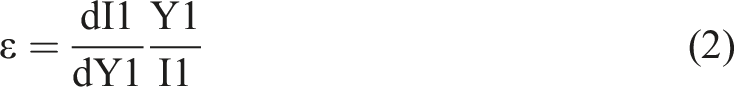
The fact that the elasticity coefficient approaches zero can be interpreted as a hysteresis structure in investments.

Another fundamental variable that determines investments is interest rates. Analyzing the sensitivity of investments to interest rate, Hall et al. (1977) stated that the Jorgenson analysis of investments on a Neoclassical basis is more valid. The lag in the effect of interest rates on investment is explained by three factors; i) delays in completing the investment: it takes about a year to design, order, and install the investment after the relative improvement in capital prices. ii) Putty-clay hypothesis: it is impossible to change the factor density in a short time as investments are generally based on fixed investments. Changes in the price of capital can only result in a change in the old capital. iii) Maturity structure of interest rates: investments realized in a given year are usually the result of investment decisions made in previous years. Therefore, investments respond to long-run interest rates and adjust capital intensity. On the other hand, besides the size of the firm, the structural state of the economy also determines the investment behavior of the firm (Khurshid, 2015). In this sense, the rate of liberalization of interest rates, the structure of investment channels and environment, and the degree of sensitivity to interest rates on a firm basis are the prominent factors. As a result of these structural differences, Sandmo (1971) observed the existence of a short-run relationship consistent with the Keynesian view, rather than a long-run stable relationship between investment and interest rates. Greene and Villanueva (1990) while there is empirical evidence in investment theory that interest rates increase the cost of capital, the degree of openness in developing countries can be seen as an exception to this structure. In economies with underdeveloped financial markets, high real interest rates can trigger investments with capital inflows. Bader and Malawi (2010) The Jordanian economy is an exceptional case where investments depend on external financing. The theoretical and empirical literature suggests that interest rates are insufficient to explain investment behavior. Therefore, the interaction between investment and interest rates is important for the detection of hysteresis. The interest rate elasticity of investments is algebraically presented in equation (3)

ε = \frac{d I 1}{d İ 1} \frac{İ 1}{I 1}

(3)

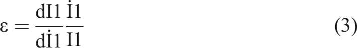
The fact that the effect of interest rates on investments is uncertain (negative or positive) in terms of theoretical and empirical literature causes the elasticity coefficient to be interpreted differently. As the elasticity coefficient moves away from zero, the response of investments to interest rate becomes more evident, while its approach to zero means that it remains unresponsive to interest rate, in other words, the hysteresis effects get stronger.

The empirical literature on hysteresis has developed in line with the theoretical foundations. Approaches to hysteresis, which is defined as temporary shocks causing permanent effects on the economy, have focused on structural breaks and asymmetric relationships. While the permanent effects of transitory shocks are analyzed by structural break tests, it is analyzed through asymmetric relationships whether the analyzed variable returns to its previous level or path in case the shocks cause the structural break to disappear. Palley (2016) argues that it is more difficult for the economy to recover structurally after decisions or shocks that cause economic change. Acemoglu and Robinson (2013) argue that changes in the distribution of income and wealth after structural changes in the economy cause asymmetry by making it more difficult for the economy to bounce back. Shen and Hong (2023) asymmetry is observed in economic variables that do not return to their previous level as a result of events that trigger geopolitical risk and uncertainty such as wars, as well as Mishra et al. (2022) provide evidence that asymmetric relationships are also seen in cost shocks as positive shocks in crude oil prices are more effective in prices than negative shocks. In this context, studies on hysteresis include studies on structural breaks in unemployment hysteresis (Blanchard & Summers, 1986; Lee & Chang, 2008; León-Ledesma & McAdam, 2004) and studies on asymmetry (Skalin & Teräsvirta, 2002; Koop & Potter, 1999). Structural breaks in trade hysteresis (Baldwin, 1988, 1990) and asymmetry (Koutmos & Martin, 2003; Fedoseeva & Werner, 2016) are prominent studies. Setterfield (1998) argues that hysteresis in investments arises from the threshold points arising from sunk costs in market entry and exit. Once this threshold for market entry is crossed, high sunk costs make it difficult to exit the market. At the same time, Dixit (1992) analyzed hysteresis in investments by taking these thresholds into account.

Literature Review

Although studies on hysteresis have intensified in the last decade, studies on investment hysteresis have remained limited. At the same time, when the empirical literature is evaluated, it is seen that the dynamics that cause hysteresis are neglected in the studies on investments. Thus, after the theoretical evaluation of investment behavior, the relationship between the findings of this study and the hysteresis literature is also presented.

In the literature, the view that there will be hysteresis effects in investments that follow a lagged adjustment process against the variables that determine investments is dominant. Dias and Shackleton (2005) analyze the investment behavior of firms under stochastic interest rates by modeling the interest elasticity of investments. When investments are evaluated in terms of interest rates, firms direct their investments towards durable investment goods when interest rates fall, while they invest in areas with high cash flows when interest rates rise. Substitutability in firms’ investment preferences provides information about hysteresis. If the firm’s investment structure is more substitutable, that is, more flexible, hysteresis effects are weaker. Belke and Göcke (2019), beyond the short-term effects of interest rates, investment behavior shaped by intertemporal optimization and expectations is also instructive for hysteresis. The expected return on investment and the fact that stochastic changes in interest rates do not have a significant impact on investments also stem from long-term effects. Since long-term interest rate expectations are shaped by short-term interest rates, an increase in short-term interest rates reduces the expected return on investment. Therefore, an increase in uncertainty in interest rates reduces the expected future return on investments and causes the entry threshold of firms to be determined with a delay compared to the exit threshold. The persistence of the volatility expectation in interest rates is a hysteresis behavior in which investments fluctuate in a much narrower path than interest rates.

In the context of firms’ entry-exit to the market; Dixit (1992), explains the theory of investment in terms of the long-run and short-run equilibrium of firms under competitive conditions and Marshall emphasizes that investments will increase if prices exceed long-run average costs. However, this process is different in real markets. Firms enter the market when prices exceed three to four times the long-run average costs. Firms’ delayed entry decision is interpreted as hysteresis. On the other hand, staying in the market under inefficient conditions due to sunk costs is also hysteresis. Dumas (1989), who emphasizes the rationality of exit decisions, explains the waiting of firms to exit the market until the threshold where losses cannot be sustained by drawing attention to a different factor. If firms exit the market early, the fact that firms are aware of the fact that they will bear sunk costs again in case the market reaches an investable point prevents exit from the market. Therefore, hysteresis causes delays in the behavior of firms, causing investments to follow a more delayed and cumbersome course than expected.

Beyond the inactivity behavior of firms and thus the slow adjustment process in economic activity, Stiglitz (1994) argues that firms’ productivity-based investment behavior can also change the growth trend during recessionary periods. During recessions, cuts in all expenditures that contribute to productivity, such as R&D and productivity-enhancing expenditures, hinder firms’ learning-by-doing process. This will result in a decline in long-run productivity and the growth trend will be adjusted to a lower path. Another alternative hypothesis explaining the long-run persistent effects of cost and productivity is the cost paradox. Hein (2015), as a proposal of the Kaleckian approach, defines the “cost paradox” as a fall in equilibrium income and hence the level of investment in the event of an increase in the profit share of firms. In the case where the cost paradox as well as the savings paradox is valid, it deepens the permanent effects on potential output. Based on this structure, the empirical literature proving the validity of the price pass-through effect and the savings paradox under cost conditions in the Turkish economy are important factors that can provide evidence for the existence of the hysteresis effect in investments. As a result, fluctuations in productivity due to cost conditions and the speed of adjustment of investments are important for the detection of hysteresis.

Pasinetti (1962) argues that there is a strong link between functional income distribution and capital formation in classical theory. Classical theory accepts that this structure in capital formation is determined by consumption and saving preferences. On the other hand, in Keynesian theory, the investment level is derived independently of consumption and saving preferences, taking into account the marginality conditions in the functional income distribution. Kaldor (1955) emphasized that marginality conditions will cause fluctuations in profit and productivity, investments and ultimately economic growth with a dynamic structure. Bruno (2005) empirically observed that even if the proportional changes in the functional income distribution are temporary, they will cause hysteresis with permanent effects. Lavoie and Stockhammer (2013) the wage-led growth strategy, which focuses on growth through investment, has begun to find more application areas globally. As it is known, wages have two basic functions in terms of production cost and being a source of demand. Existing empirical literature proves the contribution of wages to total demand, and results are obtained showing that aggregate demand and investments will also be encouraged. Rowthorn (2020) based on the savings paradox hypothesis, draws attention to the effect of wages as a component of national income on productive capital expenditure. Bassi and Lang (2016), as a result, the permanent effects of wages and thus personal disposable income on capital formation and growth are significant in terms of hysteresis effects. Warner (2014) The general view on public capital and infrastructure investments is that while accelerating growth, they also have long-run effects by contributing to productivity and level of development. Dosi et al. (2018) The effects of hysteresis are based on the deterioration of market entry dynamics and the decrease in productivity due to the decrease in aggregate demand during the crisis after prolonged economic crises. In this context, decreases in national income may cause permanent effects on investments by causing institutional deterioration. Based on this information, GDP is an important variable to better understand the hysteresis effects by causing permanent effects on the trend of economic growth.

In terms of the historical and empirical literature on hysteresis, Keynes (1936) argued that the business cycle fluctuation is driven by demand fluctuations. As a result of this fluctuation of the business cycle, the inverse movement of growth and unemployment was also clarified. Burns and Mitchell (1946) emphasized that this movement is exhibited by the nature of business cycle fluctuations (Cerra et al., 2020). Garga and Singh (2021), however, the permanent adjustment of the business cycle fluctuation to a trend different from its path is output hysteresis. Investment hysteresis is closely related to output hysteresis. Blomström et al. (1996) argue that there is not only an interaction between investment and output but also a movement from output to investment. This makes output an important variable in investment hysteresis. Fedderke (2004) argues that deterioration in the stability of output adversely affects investment. Fluctuations in investments are one of the main dynamics of output fluctuations. Investment hysteresis affects the variables that determine investments (output) and causes the hysteresis to deepen.

Blanchard and Summers (1986) argue that in the case of hysteresis, economic variables deviate from their trend and persist at these levels. This situation was experienced in unemployment in Europe in the 1980s and TFP also exhibited hysteresis behavior. Fatás and Summers (2016) show that TFP is one of the main determinants of hysteresis in the employment structure, which is the main component of output. Anzoategui et al. (2019) found that the recession process in the US economy reduced productivity and emphasized that TFP is the main dynamic in hysteresis. At the same time, Engler and Tervala (2018) conclude that the recession in Europe has persistent effects on output and TFP. Summers (2014) argues that TFP cannot improve in a state of hysteresis. If TFP fails to improve during the recovery period after the recession period, there is a decline in investments again. Girardi et al. (2020) However, in hysteresis, the effects of positive shocks can last as long as negative shocks. Positive demand shocks are found to increase GDP and investments permanently. These findings prove that the findings of this study are consistent with the empirical literature.

Data and Methodology

In the study, the methods and stages to determine the hysteresis effects in investments; First of all, structural break (hysteresis) in investments will be determined by using structural break and smooth transition structural break tests. After determining the hysteresis effects in investments with these tests, causality and asymmetric causality tests will be performed in order to analyze the basis of hysteresis effects and to offer suggestions for policymaking, and causality and asymmetric causality tests will be performed in order to suggest the structure of hysteresis effects and policy recommendations.

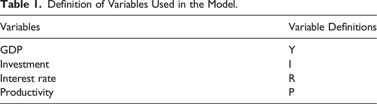
In variables, data (2005Q1: 2020Q1) source is CBRT (CBRT/EVDS), variable contents; GDP as the expression of income used in financing investments, Gross Fixed Capital formation (Investment) which includes the sum of private and public sector total investment expenditures, the ratio of total industry production index to investments (Productivity), CBRT average cost of funding (Interest rate). The variables used are presented in Table 1.

Table 1.

Definition of Variables Used in the Model.

Variables	Variable Definitions
GDP	Y
Investment	I
Interest rate	R
Productivity	P

Zivot-Andrews Structural Break Unit Root Test

Stationary analysis of time series as an econometric method is also used in the literature to detect hysteresis effects. However, based on the empirical literature, structural breaks limit the effectiveness of stationarity tests in time series. In this context, Zivot and Andrews (1992) suggested that unit root testing be done by internalizing structural breaks. Structural breaks are estimated in three models that allow structural breaks as a result of including them in the autoregressive model and internalizing them. Model A includes a level break, Model B a trend break, and Model C, a model that includes both a level and trend break, is estimated by the least squares method. The equations used in the structural break Zivot-Andrews unit root test are presented below

M o d e l A Δ y_{t} = c + α y_{t - 1} + β t + γ {D U}_{t} + \sum_{i = 1}^{k} d_{t} Δ y_{t - i} + ε

M o d e l B Δ y_{t} = c + α y_{t - 1} + β t + θ {D T}_{t} + \sum_{i = 1}^{k} d_{t} Δ y_{t - i} + ε

M o d e l C Δ y_{t} = c + α y_{t - 1} + β t + θ {D U}_{t} + γ {D T}_{t} + \sum_{i = 1}^{k} d_{t} Δ y_{t - i} + ε

Structural breaks are modeled in an autoregressive structure with the help of a dummy variable. The DU dummy variable defined for (TB) is defined as DT where slope changes are also taken into account. At this stage, T determines the prediction period, TB determines the breakout period, and λ = TB/T determines the breakpoint obtained based on the regulation region (λ ∈ (.15, .85)). The values that the dummy variables will take are; DU takes the value 1 if t > TB, 0 otherwise. Similarly, when DT is t > TB, t – TB will be 0 otherwise.

In the estimation phase, a number of regressions is estimated by the Least Squares method (T – 2) using the dummy variable used for each possible break date. As a result of the estimation, for the smallest coefficient α of the yt – 1 variable, the date when the t statistic is the smallest is accepted as the appropriate breakpoint. At this point, unit root analysis is performed without structural break. At this stage, the fact that the t statistical value calculated for α is less than the Zivot-Andrews critical values as an absolute value indicates the validity of the hypothesis that accepts the existence of a unit root without structural break. It is interpreted that the series is stationary with refraction (Zivot and Andrews, 1992, Waheed et al., 2006). The results of the Zivot-Andrews unit root test applied to the investment time series are presented in Table 2.

Table 2.

Zivot-Andrews Unit Root Test Results.

Models	Breaking Point	t Statistics	Critical Value %1	Critical Value 5%	Critical Value %10
Model A	2012Q2	−3.66	−5.34	−4.93	−4.58
Model B	2017Q3	−3.18	−4.80	−4.42	−4.11
Model C	2008Q2	−3.58	−5.57	−5.08	−4.82
Model A	Structural break model at level
Model B	Structural break model at trend
Model C	Structural break model both of trend and level

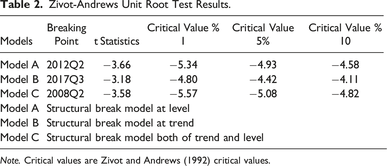
Note. Critical values are Zivot and Andrews (1992) critical values.

According to the structural break unit root test results, the H₀ basic hypothesis, which represents the existence of a unit root without structural break, is accepted in all three models at 1%, 5% and 10% significance levels. Model C, which includes level and trend, is the best model that can statistically explain the presence of hysteresis effects because it includes structural breaks in the level and trend. At this point, the existence of a unit root without a structural break in the investment time series also means that the hysteresis effect is detected.

According to the results of the Zivot-Andrews stationarity test with a structural break, there are hysteresis effects in investments. However, when we look at the structural break period, the break period coincides with the 2008 World Crisis. Crisis years include hard breaks. In this context, it becomes difficult to detect structural breaks caused by the interaction of macroeconomic variables with their path and other variables. Therefore, the use of smooth transition structural break tests in the study will provide stronger empirical evidence for the detection of hysteresis effects.

Smooth Transitions Structural Break Unit Root Test

It is a structural break test developed by Leybourne et al., (1998), in which nonlinearity is also taken into account. The strength of the smooth transition structural break test is that it can measure soft or gradual breaks instead of hard breaks while detecting structural breaks even in nonlinear time series. The smooth transition structural break test is estimated with the help of the logistic smooth transition function, which is defined as S_t, instead of the hard and sudden breaks modeled with the help of a dummy variable in other structural break tests. Logistics smooth transition function is presented below

S_{t} (γ, τ) = {[1 + \exp {- λ (t - τ T)}]}^{- 1}

Since it tests a nonlinear structure in the estimation phase, the nonlinear least squares method is used and error terms are obtained. The models from which the error terms are obtained contain three different structures. Model A considers a smooth break at the level, Model B a smooth break in the trend, while Model C considers a smooth break in both the level and the trend. The error terms equations obtained for Model A, Model B, and Model C are presented below, respectively

{\hat{v}}_{t} = y_{t} - {\hat{α}}_{1} - {\hat{α}}_{2} S_{t} (\hat{λ}, \hat{τ})

{\hat{v}}_{t} = y_{t} - {\hat{α}}_{1} - {\hat{β}}_{1} t - {\hat{α}}_{2} S_{t} (\hat{λ}, \hat{τ})

{\hat{v}}_{t} = y_{t} - {\hat{α}}_{1} - {\hat{β}}_{1} t - {\hat{α}}_{2} S_{t} (\hat{λ}, \hat{τ}) - {\hat{β}}_{2} t S_{t} (\hat{λ}, \hat{τ})

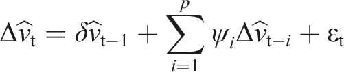
In the next step, the ADF (Augmented Dickey Fuller) test is applied to the obtained error terms. The auxiliary regression model used at this stage is presented below

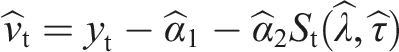
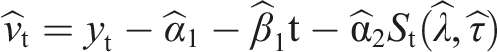
Δ {\hat{v}}_{t} = δ {\hat{v}}_{t - 1} + \sum_{i = 1}^{p} ψ_{i} Δ {\hat{v}}_{t - i} + ε_{t}

The final models that detect smooth transitional structural breaks in the time series are presented below as a smooth structural break at level Model A, a smooth structural break in trend Model B, and a smooth structural break at level and trend Model C

M o d e l A y_{t} = α_{1} + α_{2} S_{t} (λ, τ) + v_{t}

M o d e l B y_{t} = α_{1} + β_{1} t + α_{2} S_{t} (λ, τ) + v_{t}

M o d e l C y_{t} = α_{1} + β_{1} t + α_{2} S_{t} (λ, τ) + β_{2} {t S}_{t} (λ, τ) + v_{t}

The interpretation of the estimation results is done with the help of hypothesis tests.

H_{0} : δ = 0

hypothesis existence of a unit root with a smooth transition structural break is accepted. The alternative hypothesis

H_{1} : δ < 0

is interpreted as smooth structural break stationary. The alternative hypothesis is interpreted as stationary with a smooth transition structural break. Smooth transition structural break test results are presented in Table 3.

Table 3.

Smooth Transition Structural Break Test Results.

Models	Breaking Point	t Statistics	Critical Value %1	Critical Value %5	Critical Value %10
Model A (I)	2012Q4	−3.31^***	−5.09	−4.36	−4.00
Model B (I)	2012Q4	−3.32^***	−5.77	−5.05	−4.63
Model C (I)	2014Q4	−3.20^***	−6.13	−5.39	−4.99
Model A (R)	2009Q2	−.72^***	−5.09	−4.36	−4.00
Model B (R)	2009Q2	−2.10^***	−5.77	−5.05	−4.63
Model C (R)	2013Q3	−2.81^***	−6.13	−5.39	−4.99
Model A (Y)	2013Q4	−4.93^***	−5.09	−4.36	−4.00
Model B (Y)	2013Q4	−4.51^***	−5.77	−5.05	−4.63
Model C (Y)	2012Q1	−4.43***	−6.13	−5.39	−4.99
Model A (P)	2012Q3	−4.93^***	−5.09	−4.36	−4.00
Model B (P)	2012Q3	−5.73^***	−5.77	−5.05	−4.63
Model C (P)	2012Q3	−5.76^***	−6.13	−5.39	−4.99
Model A	Smooth transition structural break model at level
Model B	Smooth transition structural break model at trend
Model C	Smooth transition structural break model both of trend and level

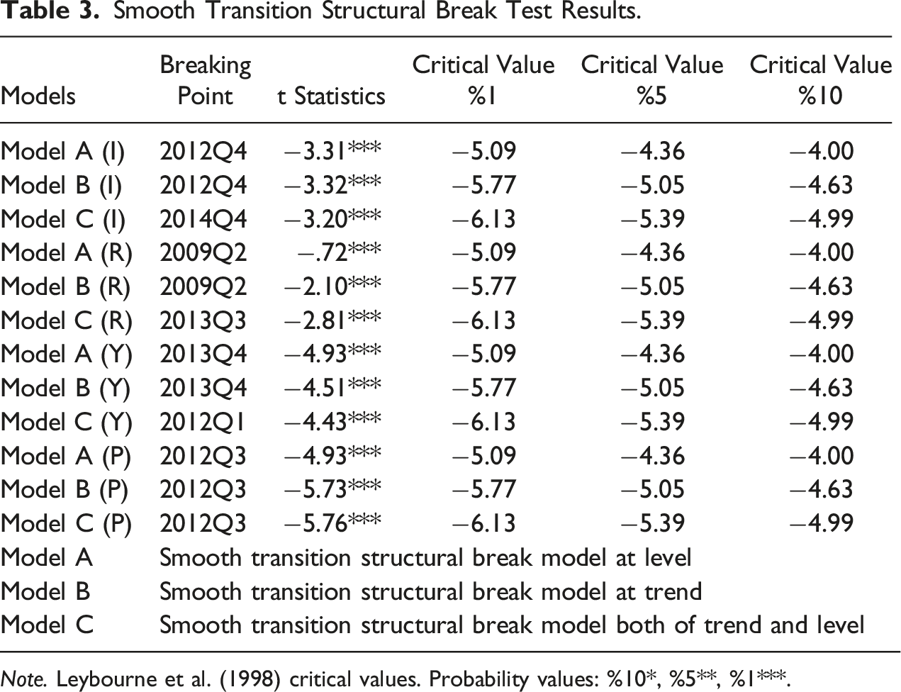
Note. Leybourne et al. (1998) critical values. Probability values: %10^*, %5^**, %1^***.

The smooth transition structural break test result is interpreted by comparing the t statistic and the critical values. If the calculated t statistic is less than the critical value chosen as the absolute value, the H₀ hypothesis cannot be rejected and this situation is interpreted as the existence of a unit root in the time series, in other words, it includes a smooth transition structural break. Based on the empirical studies in the literature, the structural break in the level and trend is determined as the model that best represents the hysteresis effects. The structural break test was applied to other variables to analyze the hysteresis effects in investments and also the basis of hysteresis effects in investments. In this context, the presence of a smooth transition structural break was found to be significant at the 1% significance level in all variables. Smooth transition structural break periods, on the other hand, occurred in 2014Q4 in investments, 2013Q3 in interest rates, 2012Q3 in GDP, and 2012Q3 in productivity.

Marjanovic and Mihajlovic (2014) argue that structural break tests are the most widely used method to detect hysteresis. In this sense, structural break tests have been used in pioneering studies in the hysteresis literature (Baldwin, 1988; Blanchard & Summers, 1986; Mitchell, 1993; Røed, 1997). As a result, the findings from structural break tests are in line with the empirical literature and point to hysteresis.

Vector Autoregressive Model (VAR)

Vector Autoregressive Models (VAR) were developed by Sims (1980) as a critique as well as an alternative to simultaneous equations. VAR models are basically a system regression model, in other words, there is more than one dependent variable. In this context, VAR models have been developed as a hybrid type of simultaneous equation models and univariate time series models. In the time series VAR model with two variables, Y1t and Y2t (this can be expanded further; Y3t, Y4t), the changes of the Y1t series over time are affected by the current and past values of the Y2t time series. On the other hand, the changes of the Y2t series throughout the time series are also affected by the current and past values of the Y1t time series. An important advantage of VAR models is their flexibility and ease of generalization. The model is expanded in a structure that also includes the delayed and moving average errors of the ARMA model, known as VARMA, designed as multivariate (Brooks, 2019). VAR model structure including error terms for Y1t and Y2t time series is defined in equation (4)

Y 1 t = β 10 + β 11 y 1 t - 1 + α 11 y 2 t - 1 + u 1 t

(4)

Y 2 t = β 20 + β 21 y 2 t - 1 + α 21 y 1 t - 1 + u 2 t .

Granger Causality Test

The existence of a causal relationship between variables in VAR models is analyzed with the Granger (1969) test. Based on the equation system (4) for the bivariate VAR model, if all lagged values of Y2t do not have a significant effect on the determination of Y1t, it is interpreted as Y2t is not the Granger cause of Y1t. The disadvantage of the Granger causality test is that it is sensitive to the lag length (Johnston & DiNardo, 1963; Baltagi, 2010). For this reason, the productivity of the model to ensure stationarity in the series before the VAR model is established. Augmented Dickey Fuller (1981), Phillips–Perron (PP) unit root tests with constant term model and constant term and trend models (ADF) were used to test the stationarity of the time series. McKinnon critical values were used to determine the stationarity levels of the time series. Unit root test results are presented in Table 4.

Table 4.

ADF and PP Unit Root Tests Results.

Variables	ADF Test		Phillips–Perron Test
Variables	Drift Model	Drift and Trend Model	Drift Model	Drift and Trend Model
Y	−.59	−1.86	−.60	−2.12
I	−1.36	−2.84	−1.43	−2.03
R	−2.74	−2.73	−2.62	−2.59
P	−2.09	−1.92	−2.16	−2.00
∆Y	−7.31	−7.25	−7.33	−7.27
∆I	−6.19	−6.16	−6.32	−6.29
∆R	−5.86	−5.80	−5.87	−5.80
∆P	−8.46	−8.46	−8.46	−8.46
Critical value %1	−3.454812	−3.992933	−3.454812	−3.992933
Critical value %5	−2.872203	−3.426809	−2.872203	−3.426809
Critical value %10	−2.572525	−3.136666	−2.572525	−3.136666

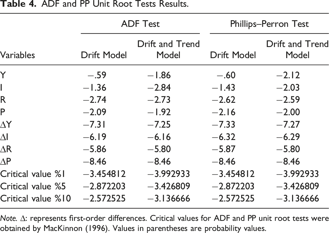
Note. ∆: represents first-order differences. Critical values for ADF and PP unit root tests were obtained by MacKinnon (1996). Values in parentheses are probability values.

As a result of the stationarity test, since GDP (Y), Investment (I), Interest (R) and Productivity (P) series are not stationary at level I (0), stationarity at first difference I (1) is achieved by applying the difference process. Determining the number of lags in autoregressive models is very important for the structure of the model. After determining the appropriate lag number as four, we proceeded to the estimation stage. Model specification; the model is stable as the characteristic polynomial roots are smaller than 1, the presence of autocorrelation is tested with the LM test and no autocorrelation problem is found, and the model does not contain changing variance, which provides sufficient conditions for statistical consistent results. The strength of the Granger causality test compared to simultaneous models is that the direction of causality can be determined bilaterally since the variables are not categorized as dependent and independent variables. Granger causality test results are presented in Table 5.

Table 5.

Granger Causality Test Results.

Causality Direction	Chi-Square (χ²)	Probability (p)	Finding
R → I	7.409520	.1158	No causality
Y → I	6.413141	.1703	No causality
P → I	4.729452	.3162	No causality

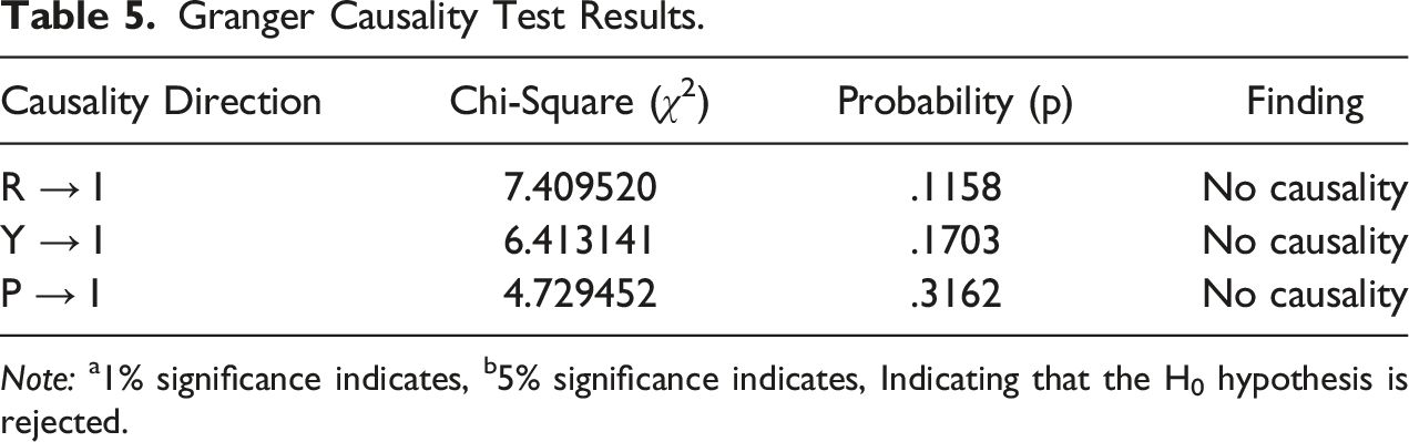
Note: ^a1% significance indicates, ^b5% significance indicates, Indicating that the H₀ hypothesis is rejected.

To determine the hysteresis effects in investments, only the direction of causality in investments has been taken into account. According to the Granger causality test results, causality from the interest rate, GDP and productivity to investments could not be determined. The Granger causality test cannot measure the different effects of positive and negative shocks in variables. The existence of asymmetrical relationships between variables in hysteresis effects has been widely detected in the empirical literature. For this reason, it would be more appropriate to use the asymmetric causality test, which takes into account the different effects of positive and negative shocks between the variables. For this reason, the asymmetric causality relationship between investment and other variables will be tested with the Hatemi-j (2012) test.

Hatemi-J Asymmetric Causality Test

Traditional causality tests used empirically in the literature by Granger (1969) and Toda-Yamamoto (1995) focus on the one-way relationship between the variables and interpret the causality results according to one-way relationships. As a result of this structure of traditional causality tests, the effect of positive and negative shocks between variables cannot be separated. As a result of not including the effect of negative and positive shocks in the model, causality in the existing asymmetrical structure cannot be determined. As an alternative to this weak structure of traditional causality tests in measuring asymmetric causality, the asymmetric causality test was developed by Hatemi-j (2012).

Yılancı and Bozoklu (2014) first analyzed the asymmetric structure between the variables, Granger and Yoon (2002) found that the positive and negative components of the time series can give different responses to positive and negative shocks. For this reason, they tested the long-run relationships with this structure, claiming that this situation would only be determined by the asymmetric cointegration test. Variables can react together and separately to certain shocks. They analyzed the long-term cointegration relationship by separating the series into cumulative positive and negative components, considering that cointegration is detected when the variables react to shocks together, while cointegration cannot be detected when they react separately. On the other hand, Hatemi-j (2012) developed the asymmetric causality test by separating the time series into cumulative positive and negative components with the same method. The fact that positive and negative shocks cause different effects and that this structure is determined will increase the effectiveness of policymaking by giving more consistent results for future forecasts.

The empirical method of the asymmetric causality test was defined with reference to the study of Hatemi-J and El-Khatib (2016). Assume that the y_t series of the m × 1 vector is analyzed, in which each element is first-order integrated into the constant and trend model. The form of the time series in the form of $y_{t} = a + b t + y_{t - 1} + ε_{t},$ is defined below

y_{t} : = [\begin{array}{c} y_{t}^{j} \\ ⋮ \\ y_{t}^{m} \end{array}], a ≔ [\begin{array}{c} a^{j} \\ ⋮ \\ a^{m} \end{array}] b ≔ [\begin{array}{c} b^{j} \\ ⋮ \\ b^{m} \end{array}] y_{0} ≔ [\begin{array}{c} y_{0}^{j} \\ ⋮ \\ y_{0}^{m} \end{array}] v e ε_{t} ≔ [\begin{array}{c} ε_{t}^{j} \\ ⋮ \\ ε_{t}^{m} \end{array}]

t = 1, 2,… T. The vector y₀ represents the initial values, while εt represents the vector of error terms. The following form is obtained by solving

y_{t} = a + b t + y_{t - 1} + ε_{t},

series with the recursive method

y_{t} = a t + \frac{t (t + 1)}{2} b + y_{0} + \sum_{i = 1}^{t} ε_{i},

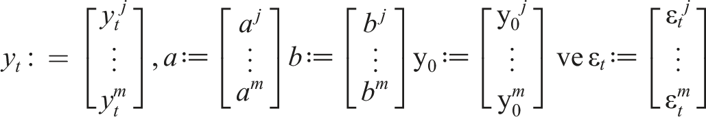
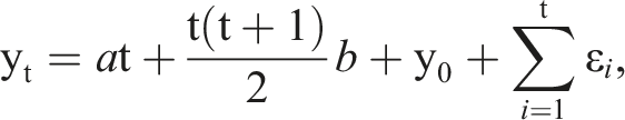
If it is necessary to take the difference d times for the series to become stationary, it will be integrated into the d order of the m-dimensional stochastic process as I(d) and solved as y_t ∼ I(d) if ∆^dy_t ∼ I (0). ∆ represents the difference operator. As a result of this process, negative and positive shocks will be defined in the form below

y_{t} = a + b t + y_{t - 1} + ε_{t} = a t + \frac{t (t + 1)}{2} b + y_{0} + \sum_{i = 1}^{t} ε_{i}^{+} + \sum_{i = 1}^{t} ε_{i}^{-},

In the next step, the cumulative forms of positive and negative shocks are defined as follows

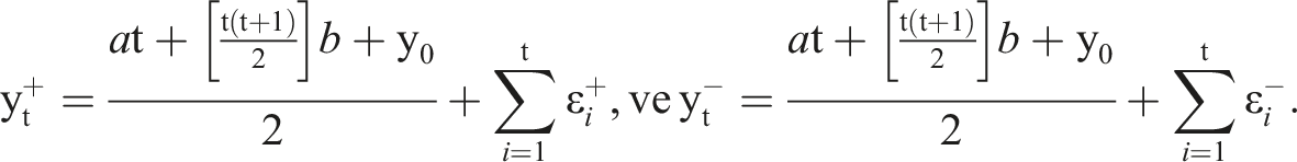
y_{t}^{+} = \frac{a t + [\frac{t (t + 1)}{2}] b + y_{0}}{2} + \sum_{i = 1}^{t} ε_{i}^{+}, v e y_{t}^{-} = \frac{a t + [\frac{t (t + 1)}{2}] b + y_{0}}{2} + \sum_{i = 1}^{t} ε_{i}^{-} .

As a result, estimation can be made with time series when cumulative negative and positive shocks are taken into account. Since asymmetric causality is structurally modeled according to a cumulative structure, it also allows to measuring the permanent effects of positive and negative shocks on the main variable. Therefore, it can be accepted as an effective test technique for measuring hysteresis effects.

As an example of the process in the asymmetric causality test, an estimation will be made in the form of a p-degree vector, namely, VAR(p), based on the assumption that the causality between the negative components is analyzed in the two-dimensional vector. The VAR model form of the vector in which the negative components are estimated will be in the form of: $y_{t}^{-} = (y_{1 t}^{-}, y_{2 t}^{-})$ and in the form of $y_{t}^{-} = ν^{-} + A_{1}^{-} y_{t - 1}^{-} + \dots + A_{p}^{-} y_{t - p}^{-} + u_{t}^{-} v^{-}$ 2 × 1 constant term vector and $u_{t}^{-}$ ise 2 × 1 is the error terms vector. The optimal lag is determined according to the point where the p information criterion is minimum. Hypothesis H₀ that k of $y_{t}^{-}$ is not a Granger cause will be tested with the Wald test for the ngg series. The Wald test is defined in the following forms

Y^{-} : = (y_{1}^{-}, \dots, y_{T}^{-}) (2 \times T) m a t r i x,

D^{-} : = (v^{-}, A_{1}^{-}, \dots, A_{p}^{-}) (2 \times (1 + 2 p)) m a t r i x,

Z_{t}^{-} : = [\begin{array}{c} 1 \\ y_{t}^{-} \\ y_{t - 1}^{-} \\ ⋮ \\ y_{t - p + 1}^{-} \end{array}] ((1 + 2 p) \times 1) m a t r i x, t = 1, \dots, f o r T,

Z^{-} : = (Z_{0}^{-}, \dots, Z_{T - 1}^{-}) ((1 + 2 p) \times T) m a t r i x,

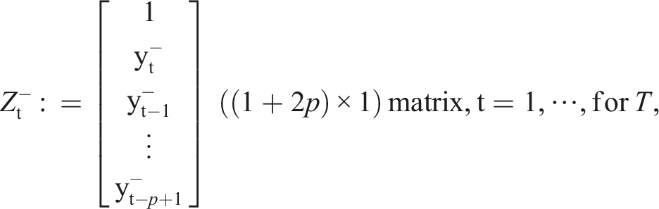
Based on the $δ^{-} : = (u_{1}^{-}, \dots, u_{T}^{-}) (2 \times T)$ matrix forms, the VAR model is expressed as $Y^{-} = D^{-} Z^{-} + δ^{-}$ like. The null hypothesis, which does not include Granger causality, is tested with the test statistics expressed in the form below

W a l d^{-} = {(C β)}^{'} {[C ({({Z^{-}}^{'} Z^{-})}^{- 1} \otimes S_{U U}^{-}) C^{'}]}^{- 1} (C β)

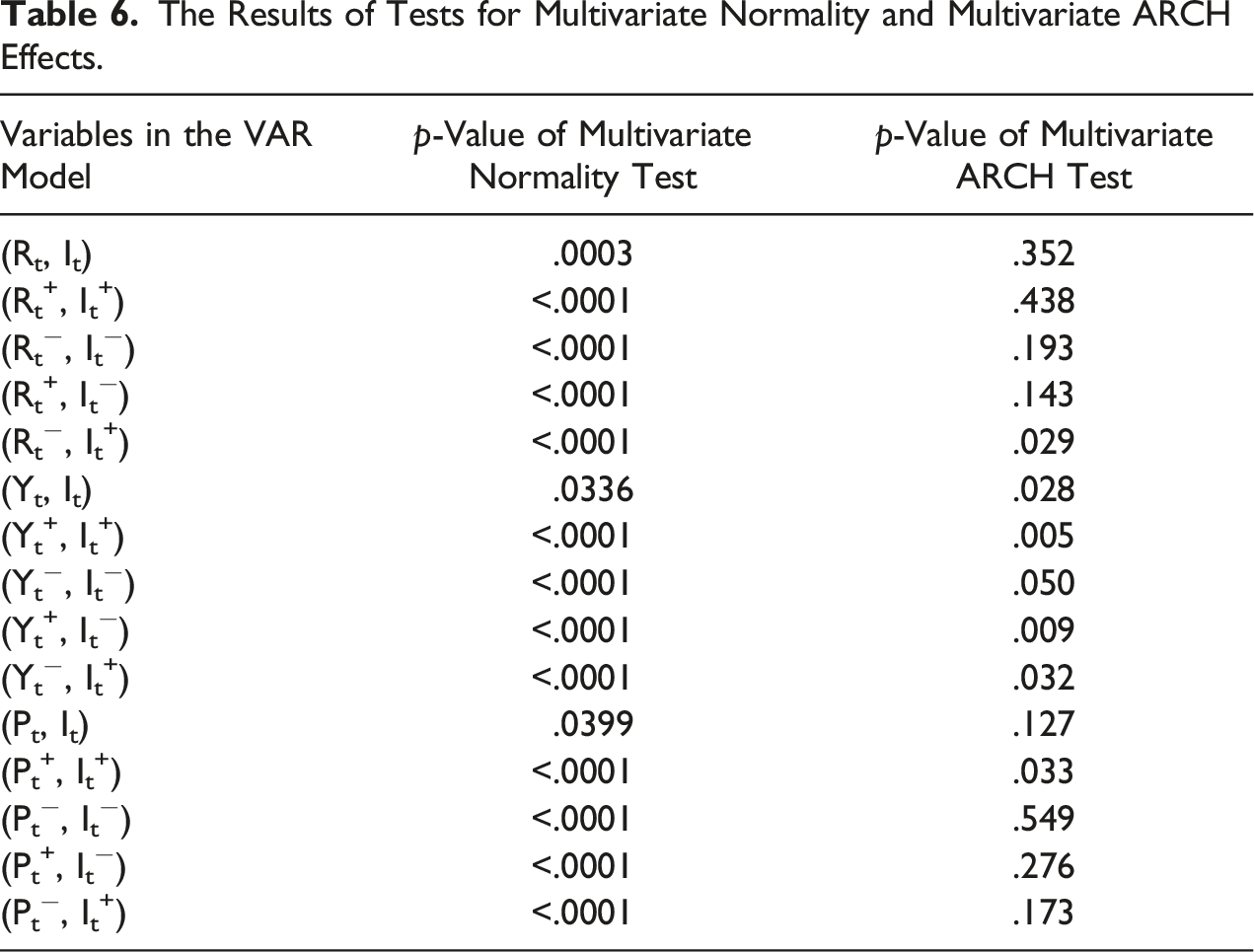
Variance-covariance matrix of the unconstrained VAR model is expressed as $S_{U}^{-} = {\hat{δ}}_{U}^{-}^{'} {\hat{δ}}_{U}^{-} / T - q$ Here q determines the estimated parameters for each VAR model. As a result, the null hypothesis of no causality is expressed as H₀: CB^- = 0

In the Granger causality test, the difference process may cause data loss in the series. For this reason, the Toda-Yamamoto (1995) test is used. The Toda-Yamamoto χ² distribution may affect the asymptotic distribution and cause the problem of non-normal distribution. Non-normality is measured by Doornik and Hansen (2008) multivariate normal distribution test and Hatemi-J multivariate ARCH (1) test.

As seen in Table 6 test results, non-normal distribution (p-value < .05) and ARCH effect (p-value < .05) are observed in the variables in the VAR model. Therefore, critical values are obtained through bootstrap simulations to ensure normal distribution. The existence of asymmetric causality is determined according to the bootstrap critical values. Asymmetric causality test results are presented in Table 7.

Table 6.

The Results of Tests for Multivariate Normality and Multivariate ARCH Effects.

Variables in the VAR Model	p-Value of Multivariate Normality Test	p-Value of Multivariate ARCH Test
(R_t, I_t)	.0003	.352
(R_t⁺, I_t⁺)	<.0001	.438
(R_t⁻, I_t⁻)	<.0001	.193
(R_t⁺, I_t⁻)	<.0001	.143
(R_t⁻, I_t⁺)	<.0001	.029
(Y_t, I_t)	.0336	.028
(Y_t⁺, I_t⁺)	<.0001	.005
(Y_t⁻, I_t⁻)	<.0001	.050
(Y_t⁺, I_t⁻)	<.0001	.009
(Y_t⁻, I_t⁺)	<.0001	.032
(P_t, I_t)	.0399	.127
(P_t⁺, I_t⁺)	<.0001	.033
(P_t⁻, I_t⁻)	<.0001	.549
(P_t⁺, I_t⁻)	<.0001	.276
(P_t⁻, I_t⁺)	<.0001	.173

Table 7.

Asymmetric Causality Test Results.

H₀	MWALD Test Statistics	1% Bootstrap Critical Values	5% Bootstrap Critical Values	10% Bootstrap Critical Values	Optimal Lag
R+ $\neq >$ I+	4.098	9.704	6.870	5.340	2
R+ $\neq >$ I−	3.304	10.806	6.862	5.104	2
R− $\neq >$ I−	2.394	14.679	7.370	5.897	2
R− $\neq >$ I+	.351	13.835	7.823	5.790	2
Y+ $\neq >$ I+	5.404	12.470	7.564	5.538	2
Y+ $\neq >$ I−	57.338^a	12.974	7.705	5.637	2
Y− $\neq >$ I−	.034	8.960	4.199	2.850	1
Y− $\neq >$ I+	91.989^a	12.810	7.511	5.936	2
P+ $\neq >$ I+	16.481^a	9.595	4.834	3.078	1
P+ $\neq >$ I−	4.903	14.501	9.789	7.372	2
P− $\neq >$ I−	1.177	9.010	4.755	3.272	1
P− $\neq >$ I+	4.651	9.294	5.635	3.927	1

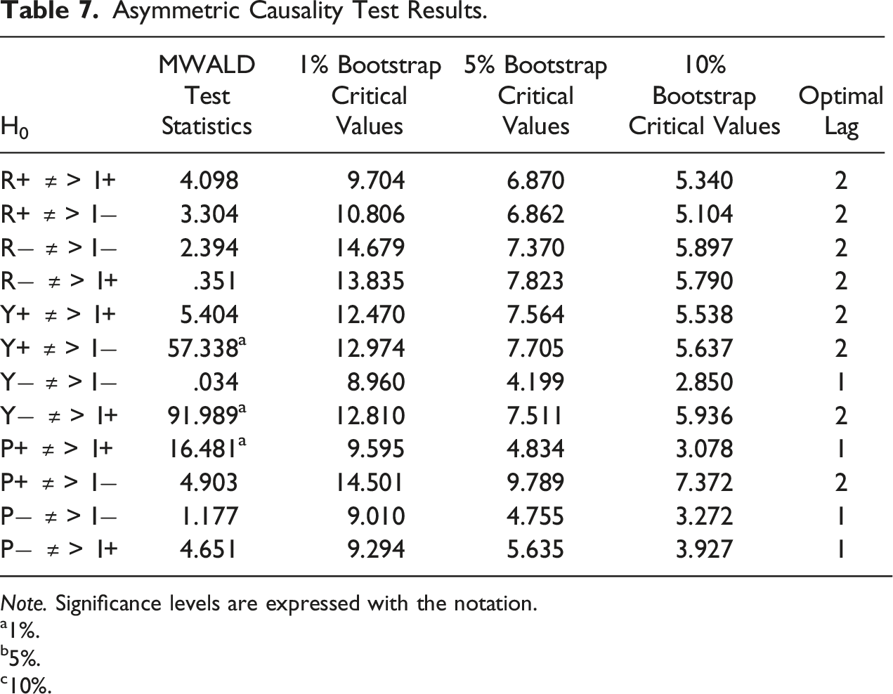
Note. Significance levels are expressed with the notation.

^a1%.

^b5%.

^c10%.

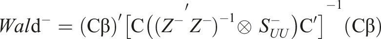
As a result of comparing the H₀ hypothesis that there is no causality in the Hatemi-J test with the bootstrap critical values, asymmetric causality is determined. If the MWALD statistic is greater than the critical values, the H0 hypothesis that there is no causality is rejected and interpreted as the presence of asymmetric causality.

In the study, the stability between positive and negative shocks in interest rate, GDP and productivity, positive and negative shocks on investments was analyzed. As a result of the asymmetric causality test, no significant relationship was found from positive and negative shocks in interest rates to investments. The causalities determined from GDP to investments are; while a stable causality was detected from positive shocks in GDP to negative shocks in investments, a stable causality relationship was found from negative shocks in GDP to positive shocks in investments. This means that investments decrease in GDP growth and increase in GDP shrinkage. This situation also provides important information about the relationship between growth and investments in the Turkish economy. The profit-oriented action of the producers in the increase in demand enables them to prefer an increase in supply by reducing the financing allocated to investments. On the other hand, the decrease in production in case of decrease in demand causes more financing to be allocated to investments and causes an increase in investments. Although this flexible structure between GDP and investments confirms the sticky wage and price model with the quantitative adjustment process of Keynesian theory, it can be concluded that shocks in GDP do not cause hysteresis effects on investments as a result of this process.

Other conclusions that can be drawn from the empirical findings are cyclical fluctuations cause fluctuations in investment financing, distorting the nature of growth and at the same time, GDP shocks do not stimulate investments with high sunk costs. The relationship between shocks in productivity and investments; while a stable causality was detected from positive shocks in productivity to positive shocks in investments, a stable causality relationship from negative shocks in productivity to negative shocks in investments could not be determined. This confirms that productivity and investments are in an asymmetric causality relationship. The asymmetric structure provides important information in terms of hysteresis effects. It is observed that positive shocks in productivity increase investments, but investments do not return to their previous level in productivity decreases. This results in productivity shocks prompting irreversible investments with high sunk costs. As a result, productivity shocks cause hysteresis effects on investments and deteriorate productivity in resource allocation.

According to the empirical findings, the inverse relationship between output and investment is explained by the cost paradox. Rowthorn (1981) argues that in the case of the cost paradox, real wage decreases seem to be a positive parameter for the firm, but they reduce aggregate demand and investment. The fact that the findings of the study are consistent with Bassi and Lang (2016) supports that the cost paradox is also effective in investment hysteresis. On the other hand, asymmetric relationships between the dynamic that triggers investments and investments are hysteresis behavior. In the empirical literature (Alfaro et al., 2018; Dixit, 1989, 1992), hysteresis is widely analyzed on the basis of asymmetric behavior. In this study, the asymmetric relationship between productivity shocks and investments as the dynamic that triggers investments proves hysteresis. However, unlike the investment hysteresis literature, this study not only identifies the asymmetric behavior of investments but also the dynamic (productivity shocks) that cause asymmetry.

Ornstein–Uhlenbeck/Vasicek Model

The Ornstein–Uhlenbeck process or Vasicek model is a Gaussian and Markovian stochastic process. Variance processes are used in the empirical literature (Bomberger, 1996; Claeys & Vašíček, 2019) to identify uncertainty conditions. Studies use the Vasicek model to measure uncertainty (Hong and Zhao, 2004; Wang and Li, 2018). According to the empirical findings, investments (1.472) have higher uncertainty than GDP (1.155), which proves the uncertainty in investments. On the other hand, productivity (5.250), which is the main dynamic of hysteresis, has the highest uncertainty. Beyond proving the uncertainty in investments, these findings also support that uncertainty in productivity deepens hysteresis (Figure 1).

Figure 1.

Investment, GDP, and productivity developments.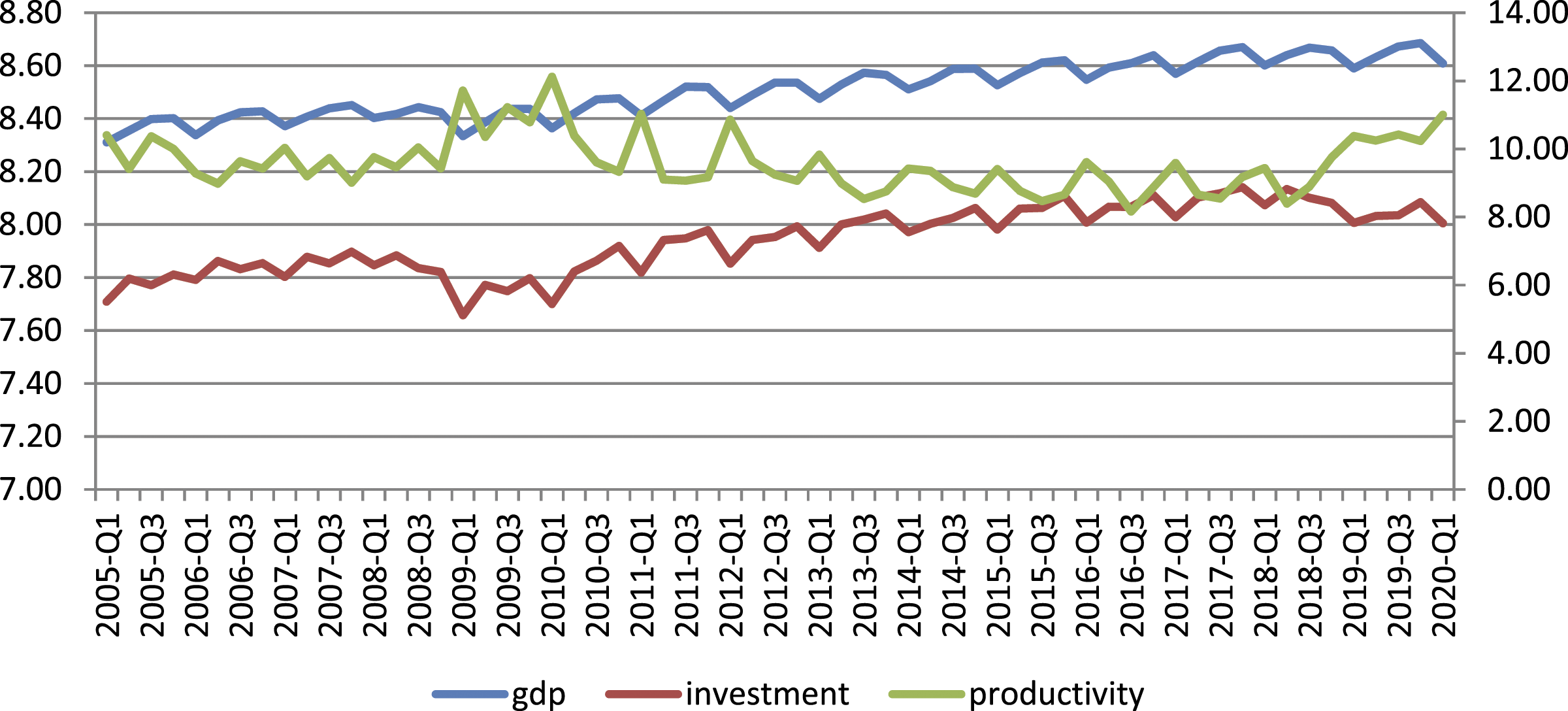

The 2008 World Crisis had a lasting impact on GDP, investment and productivity according to the degree of hysteresis. After the crisis, GDP and investment returned to their path with a lag. This proves the existence of hysteresis. On the other hand, the fact that productivity did not return to its previous level after the crisis is strong hysteresis. Moreover, despite the downward trend in productivity, temporary productivity shocks led to market entry. Transitory productivity shocks cause irreversible investments with high sunk costs and are the main dynamic of strong hysteresis.

Conclusion

The study aims to determine the validity of the hysteresis phenomenon in terms of investments in the Turkish economy. Hysteresis effects in investments can be seen in the form of structural breaks or theoretically analyzed from the responses to variables affecting investments. However, in the theoretical and empirical literature, there is a general debate on the determinants of investments in terms of interest rates, GDP and productivity. Therefore, it is necessary to identify the main determinant of investments to identify hysteresis effects and to make policy recommendations for Turkey. On the other hand, measuring the response of investments to the variable that is the main determinant of investments will provide information about the structure of hysteresis in the Turkish economy beyond the detection of hysteresis in investments. At the same time, determining which of the investment theories is valid will contribute to the gap in the empirical literature.

In the study, in addition to the structural break tests widely used in the empirical literature to detect hysteresis, the relationship with the variables that are theoretically determinants of investments (interest rate, GDP, productivity) was analyzed. According to the findings obtained from the structural break tests, the existence of a structural break in investments was detected. These findings are consistent with the empirical literature and point to hysteresis. In the next stage, the traditional causality test (Granger) was used to identify the determinants of investments. However, no causality was found from the interest rate, GDP and productivity to investments. As is known, apart from structural breaks, another structural form of hysteresis is asymmetric relationships. At this point, asymmetric relationships between investments and the determinants of investments (interest rate, GDP, productivity) were analyzed. According to the findings of the asymmetric causality test, there is no relationship between interest rates and investments, there is an inverse relationship between investments and GDP, and asymmetric causality is found between productivity and investments. The asymmetric relationship proves the validity of hysteresis in investments. Productivity is the determinant of investments and the dynamic that causes hysteresis. The fact that investments have higher uncertainty than GDP proves the uncertainty in investments. Moreover, the fact that productivity shocks, which are the main dynamics of hysteresis, contain very high uncertainty increases the uncertainty in investments and deepens hysteresis.

There are important issues regarding the empirical approach and the findings of the study. Another important finding from the asymmetric causality test is that GDP and investments have an inverse causality relationship. While investments decrease in periods when GDP increases, investments increase in periods when GDP decreases. This behavior in investments can be explained by the cost paradox based on Post Keynes. It is concluded that despite the increase in output, the decline in real income due to the chronic inflation problem in the Turkish economy reduces aggregate demand and investment demand. The cost paradox is another dynamic that deepens the hysteresis in investments. On the other hand, in the Post Keynes view, profits are the determinant of investments. The fact that productivity conditions (Geamănu, 2011), another proxy of profits, increase investments supports the validity of the Post Keynes view in the investment behavior of the Turkish economy. Moreover, the fact that other structural breaks in GDP (2012Q1) and productivity (2012Q3) occurred before the structural break in investment (2014Q4) supports these findings. As a result, in addition to identifying the investment hysteresis, the study also identifies the determinants of investments, which school of economics is valid in investment behavior and the dynamics that cause hysteresis, unlike the empirical literature.

The points to be taken into consideration in policymaking are that since no causality relationship between interest rates and investments has been detected, measures should be taken to create a favorable investment environment in order for reasonable interest rate conditions to mobilize investments. Since the inverse relationship between GDP and investments stems from the cost paradox, measures should be taken to ensure income distribution in output increases. The asymmetric relationship between investment and productivity has shown that investment volume does not decrease in periods of declining productivity. In terms of investments, this process causes inefficiency in resource allocation. Therefore, policymakers should take measures to regulate irreversible investments with a regulatory financing policy in periods of temporary productivity shocks.

Footnotes

Declaration of Conflicting Interests

The author(s) declared no potential conflicts of interest with respect to the research, authorship, and/or publication of this article.

Funding

The author(s) received no financial support for the research, authorship, and/or publication of this article.

Ethical Approval

This article does not contain any studies with human participants performed by any of the authors.

ORCID iD

Koray Yildirim

References

Acemoglu

Robinson

J. A.

(2013). Economics versus politics: Pitfalls of policy advice. Voprosy Ekonomiki, 27(12), 4–28. https://doi.org/10.32609/0042-8736-2013-12-4-28

Adler

Duval

M. R. A.

Furceri

Çelik

S. K.

Koloskova

Poplawski-Ribeiro

(2017). Gone with the headwinds: Global productivity. International Monetary Fund.

Akkina

K. R.

Celebi

M. A.

(2002). The determinants of private fixed investment and the relationship between public and private capital accumulation in Turkey. The Pakistan Development Review, 41(3), 243–254. https://doi.org/10.30541/v41i3pp.243-254

Alfaro

Cunat

Fadinger

Liu

(2018). The real exchange rate, innovation and productivity: Heterogeneity, asymmetries and hysteresis (No. w24633). National Bureau of Economic Research.

Altıntaş

Taban

(2011). Twin deficit problem and Feldstein-Horioka hypothesis in Turkey: ARDL bound testing approach and investigation of causality. International Research Journal of Finance and Economics, 74(1), 30–45.

Anzoategui

Comin

Gertler

Martinez

(2019). Endogenous technology adoption and R&D as sources of business cycle persistence. American Economic Journal: Macroeconomics, 11(3), 67–110. https://doi.org/10.1257/mac.20170269

Arestis

(1996). Post-keynesian economics: Towards coherence. Cambridge Journal of Economics, 20(1), 111–135. https://doi.org/10.1093/oxfordjournals.cje.a013604

Baker

S. R.

Bloom

Davis

S. J.

(2016). Measuring economic policy uncertainty. The Quarterly Journal of Economics, 131(4), 1593–1636. https://doi.org/10.1093/qje/qjw024

Baldwin

(1988). Hysteresis in import prices: The beachhead effect, The American Economic Review, 78(4), 773–785. https://www.jstor.org/stable/1811174

10.

Baldwin

(1990). Hysteresis in trade. In Hysteresis effects in economic models (pp. 19–34). Physica-Verlag HD.

11.

Baldwin

Krugman

(1989). Persistent trade effects of large exchange rate shocks. The Quarterly Journal of Economics, 104(4), 635–654. https://doi.org/10.2307/2937860

12.

Ball

(2015). Monetary policy for a high-pressure economy. Center on Budget and Policy Priorities.

13.

Baltagi

B. H.

(2010). Solutions manual for econometrics. Springer.

14.

Bassi

Lang

(2016). Investment hysteresis and potential output: A post-Keynesian–Kaleckian agent-based approach. Economic Modelling, 52, 35–49. https://doi.org/10.1016/j.econmod.2015.06.022

15.

Belke

A. H.

Göcke

(2019). Interest rate hysteresis in macroeconomic investment under uncertainty. Institute of Labor Economics.

16.

Benhabib

Spiegel

M. M.

(2000). The role of financial development in growth and investment. Journal of Economic Growth, 5(4), 341–360. https://doi.org/10.1023/a:1026599402490

17.

Blanchard

O. J.

Summers

L. H.

(1986). Hysteresis and the European unemployment problem. NBER Macroeconomics Annual, 1, 15–78. https://doi.org/10.1086/654013

18.

Blomström

Lipsey

R. E.

Zejan

(1996). Is fixed investment the key to economic growth? The Quarterly Journal of Economics, 111(1), 269–276. https://doi.org/10.2307/2946665

19.

Bomberger

W. A.

(1996). Disagreement as a measure of uncertainty. Journal of Money, Credit and Banking, 28(3), 381–392. https://doi.org/10.2307/2077981

20.

Brooks

(2019). Introductory econometrics for finance. Cambridge University Press.

21.

Bruno

(2005, September). Income repartition and hysteresis in a post-Keynesian growth model. In Conference The Keynesian Legacy in Macroeconomic Modeling (pp. 16–17).

22.

Burns

A. F.

Mitchell

W. C.

(1946). Measuring business cycles. National Bureau of Economic Research. Available at: https://ideas.repec.org/b/nbr/nberbk/burn46-1.html

23.

Carruth

Dickerson

Henley

(2000). What do we know about investment under uncertainty? Journal of Economic Surveys, 14(2), 119–154. https://doi.org/10.1111/1467-6419.00107

24.

Cerqueira

P. A.

Martins

(2009). Measuring the determinants of business cycle synchronization using a panel approach. Economics Letters, 102(2), 106–108. https://doi.org/10.1016/j.econlet.2008.11.016

25.

Cerra

M. V.

Fatás

Saxena

M. S. C.

(2020). Hysteresis and business cycles. International Monetary Fund.

26.

Cerra

Fatas

Saxena

(2023). Hysteresis and business cycles. Journal of Economic Literature, 61(1), 181–225. https://doi.org/10.1257/jel.20211584

27.

Claeys

Vašíček

(2019). Transmission of uncertainty shocks: Learning from heterogeneous responses on a panel of EU countries. International Review of Economics and Finance, 64, 62–83. https://doi.org/10.1016/j.iref.2019.05.012

28.

Clark

P. K.

Greenspan

Goldfeld

S. M.

Clark

(1979). Investment in the 1970s: Theory, performance, and prediction. Brookings Papers on Economic Activity, 1979(1), 73–124. https://doi.org/10.2307/2534305

29.

Dias

J. C.

Shackleton

M. B.

(2005). Investment hysteresis under stochastic interest rates. Lancaster University Management School. Working Paper 2005/060.

30.

Dickey

D. A.

Fuller

W. A.

(1981). Likelihood ratio statistics for autoregressive time series with a unit root. Econometrica, 49(4), 1057–1072. https://doi.org/10.2307/1912517

31.

Dixit

(1989). Hysteresis, import penetration, and exchange rate pass-through. The Quarterly Journal of Economics, 104(2), 205–228. https://doi.org/10.2307/2937845

32.

Dixit

(1992). Investment and hysteresis. Journal of Economic Perspectives, 6(1), 107–132. https://doi.org/10.1257/jep.6.1.107

33.

Doornik

J. A.

Hansen

(2008). An omnibus test for univariate and multivariate normality. Oxford Bulletin of Economics and Statistics, 70(1), 927–939. https://doi.org/10.1111/j.1468-0084.2008.00537.x

34.

Dosi

Pereira

M. C.

Roventini

Virgillito

M. E.

(2018). Causes and consequences of hysteresis: Aggregate demand, productivity, and employment. Industrial and Corporate Change, 27(6), 1015–1044. https://doi.org/10.1093/icc/dty010

35.

Dumas

(1989). Perishable investment and hysteresis in capital formation (p. w2930). NBER Working Paper.

36.

Engler

Tervala

(2018). Hysteresis and fiscal policy. Journal of Economic Dynamics and Control, 93, 39–53. https://doi.org/10.1016/j.jedc.2018.02.002

37.

Ethem

E. S. E. N.

YILDIRIM

Kostakoğlu

S. F.

(2012). Feldstein-horioka hipotezinin Türkiye ekonomisi için sınanması: ARDL modeli uygulaması. Eskişehir Osmangazi Üniversitesi İktisadi Ve İdari Bilimler Dergisi, 7(1), 251–267. https://dergipark.org.tr/tr/pub/oguiibf/issue/5717/76525

38.

Fatás

Summers

L. H.

(2016). The permanent effects of fiscal consolidations, Journal of International Economics, 112, 238–250. No. w22374. https://doi.org/10.1016/j.jinteco.2017.11.007

39.

Fedderke

(2004). Investment in fixed capital stock: Testing for the impact of sectoral and systemic uncertainty. Oxford Bulletin of Economics and Statistics, 66(2), 165–187. https://doi.org/10.1046/j.0305-9049.2003.00078.x

40.

Fedoseeva

Werner

L. M.

(2016). How linear is pricing-to-market? Empirical assessment of hysteresis and asymmetry of PTM. Empirical Economics, 50(3), 1065–1090. https://doi.org/10.1007/s00181-015-0957-4

41.

Fisher

A. C.

(2000). Investment under uncertainty and option value in environmental economics. Resource and Energy Economics, 22(3), 197–204. https://doi.org/10.1016/s0928-7655(00)00025-7

42.

Furceri

Kilic Celik

Jalles

J. T.

Koloskova

(2021). Recessions and total factor productivity: Evidence from sectoral data. Economic Modelling, 94, 130–138. https://doi.org/10.1016/j.econmod.2020.09.025

43.

Garga

Singh

S. R.

(2021). Output hysteresis and optimal monetary policy. Journal of Monetary Economics, 117, 871–886. https://doi.org/10.1016/j.jmoneco.2020.06.005

44.

Geamănu

(2011). Economic efficiency and profitability, Arad-Seria Ştiinţe Economice (21(2), pp. 116–119). Studia Universitatis Vasile Goldiş.

45.

Ghura

Goodwin

(2000). Determinants of private investment: A cross-regional empirical investigation. Applied Economics, 32(14), 1819–1829. https://doi.org/10.1080/000368400425044

46.

Girardi

Paternesi Meloni

Stirati

(2020). Reverse hysteresis? Persistent effects of autonomous demand expansions. Cambridge Journal of Economics, 44(4), 835–869. https://doi.org/10.1093/cje/beaa009

47.

Gordon

M. J.

(1992). The neoclassical and a post Keynesian theory of investment. Journal of Post Keynesian Economics, 14(4), 425–443. https://doi.org/10.1080/01603477.1992.11489909

48.

Granger

Yoon

(2002). Hidden cointegration. University of California. Department of Economics Çalışma Raporu.

49.

Granger

C. W. J.

(1969). Investigating causal relations by econometric models and crossspectral methods. Econometrica, 37(3), 424–438. https://doi.org/10.2307/1912791

50.

Greene

Villanueva

(1990). Determinants of private investment in LDCs. Finance and Development, 27(4), 40.

51.

Hall

R. E.

Sims

C. A.

Modigliani

Brainard

(1977). Investment, interest rates, and the effects of stabilization policies. Brookings Papers on Economic Activity, 1977(1), 61–121. https://doi.org/10.2307/2534257

52.

Hatemi-j

(2012). Asymmetric causality tests with an application. Empirical Economics, 43(1), 447–456. https://doi.org/10.1007/s00181-011-0484-x

53.

Hatemi-J

El-Khatib

(2016). An extension of the asymmetric causality tests for dealing with deterministic trend components. Applied Economics, 48(42), 4033–4041. https://doi.org/10.1080/00036846.2016.1150950

54.

Hein

(2015). The principle of effective demand: Marx, Kalecki, Keynes and beyond. No. 60/2015). Working paper.

55.

Hong

Zhao

(2004). Out-of-sample performance of discrete-time spot interest rate models. Journal of Business and Economic Statistics, 22(4), 457–473. https://doi.org/10.1198/073500104000000433

56.

Hong

Wang

Pan

(2022). Relationship between the news-based categorical economic policy uncertainty and US GDP: A mixed-frequency granger-causality analysis. Finance Research Letters, 48, 103024. https://evds2.tcmb.gov.tr/index.php?/evds/serieMarketTCMB (Accessed: 20.06.2021).

57.

Hong

Feng

Wang

(2022). Evaluating the importance of monetary policy uncertainty: The long-and short-term effects and responses. Evaluation Review, 47(2), 264–286. https://doi.org/10.1177/0193841x221124434

58.

Isham

Kaufmann

(1999). The forgotten rationale for policy reform: The productivity of investment projects. The Quarterly Journal of Economics, 114(1), 149–184. https://doi.org/10.1162/003355399555972

59.

Johnston

DiNardo

(1963). Econometric methods. International Monetary Fund.

60.

Jordà

Ò.

Singh

S. R.

Taylor

A. M.

(2020). The long-run effects of monetary policy (No. w26666). National Bureau of Economic Research.

61.

Jorgenson

D. W.

(1963). Capital theory and investment behavior. The American Economic Review, 53(2), 247–259.

62.

Kaldor

(1955). Alternative theories of distribution. The Review of Economic Studies, 23(2), 83–100. https://doi.org/10.2307/2296292

63.

Kaygısız

A. D.

Dilek

G. Ö. Z. E.

Kösekahyaoğlu

(2016). Türkiye’de Tasarruf, yatırım, cari açık ve büyüme: 1980–2014 dönemi üzerine bir nedensellik ilişkisi analizi. Çankırı Karatekin Üniversitesi Sosyal Bilimler Enstitüsü Dergisi, 7(1), 273–300.

64.

Keynes

J. M.

1883-1946 . (1936). The general theory of employment, interest and money. Macmillan.

65.

Khan

M. S.

Reinhart

C. M.

(1990). Private investment and economic growth in developing countries. World Development, 18(1), 19–27. https://doi.org/10.1016/0305-750x(90)90100-c

66.

Kinnon

M. R.

(1973). Money and capital in economic development. The Brookings Institution.

67.

Koop

Potter

S. M.

(1999). Dynamic asymmetries in US unemployment. Journal of Business and Economic Statistics, 17(3), 298–312. https://doi.org/10.2307/1392288

68.

Koutmos

Martin

A. D.

(2003). Asymmetric exchange rate exposure: Theory and evidence. Journal of International Money and Finance, 22(3), 365–383. https://doi.org/10.1016/s0261-5606(03)00012-3

69.

Lavoie

Stockhammer

(2013). Wage-led growth: Concept, theories and policies. In Wage-led growth (pp. 13–39). Palgrave Macmillan.

70.

Lee

C. C.

Chang

C. P.

(2008). Unemployment hysteresis in OECD countries: Centurial time series evidence with structural breaks. Economic Modelling, 25(2), 312–325. https://doi.org/10.1016/j.econmod.2007.06.002

71.

León-Ledesma

M. A.

McAdam

(2004). Unemployment, hysteresis and transition. Scottish Journal of Political Economy, 51(3), 377–401. https://doi.org/10.1111/j.0036-9292.2004.00311.x

72.

Levine

Renelt

(1992). A sensitivity analysis of cross-country growth regressions (pp. 942–963). The American Economic Review.

73.

Leybourne

Newbold

Vougas

(1998). Unit roots and smooth transitions. Journal of Time Series Analysis, 19(1), 83–97. https://doi.org/10.1111/1467-9892.00078

74.

Liang

Wei

Zhang

(2020). Uncertainty and crude oil market volatility: New evidence. Applied Economics, 52(27), 2945–2959. https://doi.org/10.1080/00036846.2019.1696943

75.

Lopez

Mott

(1999). Kalecki versus Keynes on the determinants of investment. Review of Political Economy, 11(3), 291–301. https://doi.org/10.1080/095382599107020

76.

MacKinnon

J. G.

(1996). Numerical distribution functions for unit root and cointegration tests. Journal of Applied Econometrics, 11(6), 601–618.

77.

Malawi

Bader

(2010). The impact of interest rate on investment in Jordan: A cointegration analysis. Journal of King Abdulaziz University-Economics and Administration, 24(1), 199–209. https://doi.org/10.4197/eco.24-1.6

78.

Marjanovic

Mihajlovic

(2014). Analysis of hysteresis in unemployment rates with structural breaks: The case of selected European countries. Engineering Economics, 25(4), 378–386. https://ssrn.com/abstract=3774791

79.

Mishra

A. K.

Ghate

Renganathan

Kennet

J. J.

Rajderkar

N. P.

(2022). Rolling, recursive evolving and asymmetric causality between crude oil and gold prices: Evidence from an emerging market. Resources Policy, 75, 102474. https://doi.org/10.1016/j.resourpol.2021.102474

80.

Mitchell

W. F.

(1993). Testing for unit roots and persistence in OECD unemployment rates. Applied Economics, 25(12), 1489–1501. https://doi.org/10.1080/00036849300000153

81.

Modigliani

Miller

M. H.

(1958). The cost of capital, corporation finance and the theory of investment. The American Economic Review, 48(3), 261–297.

82.

Palley

(2016). A theory of economic policy lock-in and lock-out via hysteresis: Rethinking economists’ approach to economic policy. Economics discussion papers, No 2016-50. Kiel Institute for the World Economy.

83.

Pasinetti

L. L.

(1962). Rate of profit and income distribution in relation to the rate of economic growth. The Review of Economic Studies, 29(4), 267–279. https://doi.org/10.2307/2296303

84.

Piscitelli

Cross

Grinfeld

Lamba

(2000). A test for strong hysteresis. Computational Economics, 15(1/2), 59–78. https://doi.org/10.1023/a:1008638827537

85.

Poitras

(2002). The philosophy of investment: A post Keynesian perspective. Journal of Post Keynesian Economics, 25(1), 105–121. https://doi.org/10.1080/01603477.2002.11051342

86.

Røed

(1997). Hysteresis in unemployment. Journal of Economic Surveys, 11(4), 389–418. https://doi.org/10.1111/1467-6419.00040

87.

Rowthorn

(2020). The Godley–Tobin lecture*: Keynesian economics–back from the dead? Review of Keynesian Economics, 8(1), 1–20. https://doi.org/10.4337/roke.2020.01.01

88.

Rowthorn

R. E.

(1981). Demand, real wages and economic growth. Thames Polytechnic.

89.

Sandmo

(1971). Investment and the rate of interest. Journal of Political Economy, 79(6), 1335–1345. https://doi.org/10.1086/259839

90.

Schmitt-Grohé

Uribe

Woodford

(2012). International macroeconomics. Textbook manuscript. Columbia University.

91.

Setterfield

(1998). Adjustment asymmetries and hysteresis in simple dynamic models. The Manchester School, 66(3), 283–301. https://doi.org/10.1111/1467-9957.00102

92.

Shaw

E. S.

(1973). Financial deepening in economic development. Oxford University Press.

93.

Shen

Hong

(2023). Can geopolitical risks excite Germany economic policy uncertainty: Rethinking in the context of the Russia-Ukraine conflict. Finance Research Letters, 51, 103420. https://doi.org/10.1016/j.frl.2022.103420

94.

Sims

C. A.

(1980). Comparison of interwar and postwar business cycles: Monetarism reconsidered. The American Economic Review, 70(2), 250–257.

95.

Skalin

Teräsvirta

(2002). Modeling asymmetries and moving equilibria in unemployment rates. Macroeconomic Dynamics, 6(2), 202–241. https://doi.org/10.1017/s1365100502031024

96.

Steigum

Jr. (1983). A financial theory of investment behavior. Econometrica, 51(3), 637–645. https://doi.org/10.2307/1912151

97.

Stiglitz

J. E.

(1994). Endogenous growth and cycles. Innovation in Technology, Industries, and Institutions (pp. 121–156).

98.

Summers

L. H.

(2014). US economic prospects: Secular stagnation, hysteresis, and the zero lower bound. Business Economics, 49(2), 65–73. https://doi.org/10.1057/be.2014.13

99.

Suyuan

Khurshid

(2015). The effect of interest rate on investment; Empirical evidence of Jiangsu province, China. Journal of International Studies, 8(1), 81–90. https://doi.org/10.14254/2071-8330.2015/8-1/7

100.

Tervala

(2021). Hysteresis and the welfare costs of recessions. Economic Modelling, 95, 136–144. https://doi.org/10.1016/j.econmod.2020.12.012

101.

Tervala

Watson

(2022). Hysteresis and fiscal stimulus in a recession. Journal of International Money and Finance, 124, 102614. https://doi.org/10.1016/j.jimonfin.2022.102614

102.

Toda

H. Y.

Yamamoto

(1995). Statistical inference in vector autoregressions with possibly integrated processes. Journal of Econometrics, 66(1–2), 225–250. https://doi.org/10.1016/0304-4076(94)01616-8

103.

Uçan

Öztürk

Ö.

(2011). Financial determinants of investment for Turkey. Journal of Economic and Social Studies, 1(1), 83–110. https://doi.org/10.14706/jecoss11117

104.

Waheed

Alam

Ghauri

S. P.

(2006). Structural breaks and unit root: Evidence from Pakistani macroeconomic time series (December 15, 2006), SSRN Electronic Journal. Available at: http://dx.doi.org/10.2139/ssrn.963958

105.

Wang

P. G.

Chen

Kong

(2018). High level expression and glycosylation of recombinant Mycobacterium tuberculosis Ala-Pro-rich antigen in Pichia pastoris. Protein Expression and Purification, 150, 67–71. https://doi.org/10.1016/j.pep.2018.05.004

106.

Warner

M. A. M.

(2014). Public investment as an engine of growth (No. 14-148). International Monetary Fund.

107.

(2000). Financial development, investment, and economic growth. Economic Inquiry, 38(2), 331–344. https://doi.org/10.1111/j.1465-7295.2000.tb00021.x

108.

Yilanci

Bozoklu

Ş.

(2014). Türk sermaye piyasasında fiyat ve işlem hacmi ilişkisi: Zamanla değişen asimetrik nedensellik analizi. Ege Akademik Bakis (Ege Academic Review), 14(2), 211. https://doi.org/10.21121/eab.2014218052

109.

Zivot

Andrews

D. W. K.

(2002). Further evidence on the great crash, the oil-price shock, and the unit-root hypothesis. Journal of Business and Economic Statistics, 20(1), 25–44. https://doi.org/10.1198/073500102753410372

Investment Hysteresis: An Empirical Essay Turkish Case

Abstract

Keywords

Introduction

Theoretical Framework

Literature Review

Data and Methodology

Zivot-Andrews Structural Break Unit Root Test

Smooth Transitions Structural Break Unit Root Test

Vector Autoregressive Model (VAR)

Granger Causality Test

Hatemi-J Asymmetric Causality Test

Ornstein–Uhlenbeck/Vasicek Model

Conclusion

Footnotes

Declaration of Conflicting Interests

Funding

Ethical Approval

ORCID iD

References