Vector autoregressive-based Granger causality test in the presence of instabilities

Abstract

In this article, we review Granger causality tests that are robust to the presence of instabilities in a vector autoregressive framework. We also introduce the gcrobustvar command, which illustrates the procedure in Stata. In the presence of instabilities, the Granger causality robust test is more powerful than the traditional Granger causality test.

1 Introduction

Vector autoregressive (VAR) models have played an important role in macroeconomic analysis since Sims (1980). A VAR is a multiequation, multivariable linear model where each variable is in turn explained by its own lagged values as well as current and past values of the remaining variables. Compared with a univariate autoregression, VARs provide both a systematic way to capture the rich dynamics in multiple time series and a coherent, credible approach to forecasting.

Granger (1969) causality is a useful tool for characterizing the dependence among time series in reduced-form VARs, and Granger causality test statistics are widely used to examine whether lagged values of one variable help to predict another variable—see Stock and Watson (2001).

However, VAR analyses in macroeconomic data face important practical challenges: economic time-series data are prone to instabilities (see Stock and Watson [1996, 1999, 2003, 2006]; Rossi [2013]; Clark and McCracken [2006]), and VAR estimates may also be prone to instabilities (see Boivin and Giannoni [2006], Kozicki and Tinsley [2001], and Cogley and Sargent [2001, 2005]).

Thus, given the widespread use of VARs and the evidence of instabilities, it is potentially important to allow for changes over time when doing VAR-based statistical inference. As demonstrated in Rossi (2005), because the traditional Granger causality test assumes stationarity, it is not reliable in the presence of instabilities and may lead to incorrect inference.

In this article, we present the gcrobustvar command, which illustrates how to test Granger causality in a way that is robust to the presence of instabilities. The test is based on methodologies developed by Rossi (2005) and includes the robust versions of the mean and exponential Wald tests (Andrews and Ploberger 1994), the Nyblom (1989) test, and the Quandt (1960) and Andrews (1993) quasilikelihood-ratio tests. In the presence of instabilities, the Granger causality robust tests are more powerful than the traditional Granger causality test. The tests can also be used to find the point in time in which Granger causality either appears or breaks down in the data. In addition, the test is valid for reduced-form VAR models and VAR-based direct multistep (VAR– LP) forecasting models. The former assume homoskedastic idiosyncratic shocks, while the latter are estimated via local projections (LP) (see Jord`a [2005]) and hence assume heteroskedastic and serially correlated idiosyncratic shocks.

We first introduce the tests and then present the commands that implement them. Then, we illustrate the empirical implementation of the robust Granger causality tests using a three-variable (inflation, unemployment, and interest rate) VAR model with four lags as in Stock and Watson (2001), as well as a direct multistep VAR–LP forecasting model. Finally, we compare the results with those based on a traditional Granger causality test.

The remainder of this article is organized as follows. Section 2 describes the theoretical framework and the Granger causality robust tests. Section 3 introduces the gcrobustvar command, which implements the Granger causality robust tests in Stata. Section 4 applies the Granger causality robust tests in the three-variable VAR and compares the results with the traditional Granger causality test. Section 5 applies the Granger causality robust tests in the direct multistep VAR–LP forecasting model.

2 VAR-based Granger causality test in the presence of instabilities

2.1 Motivation

In the presence of instabilities, as shown in Rossi (2005), traditional Granger causality tests may have no power. Consider one of the equations in a two-variable VAR with one lag and fixed prediction horizon h, for example: $y_{\text{t}+\text{h}}={\beta }_{\text{t}}{x}_{\text{t}-\text{1}}+\rho y_{\text{t}-\text{1}}+{\epsilon }_{\text{t}+\text{h},}\hspace{0.17em}t=\text{ 2},\text{3}, . . . , T.$ For simplicity, we assume that $x_{\text{t}}{{ }_{-}}_{\text{1}}, {\epsilon }_{\text{t}}{{ }_{+}}_{\text{h}}\hspace{0.17em}\stackrel{\text{i}.\text{i}.\text{d}}{\sim }\hspace{0.17em}N\left(0,1\right)$ and $x_{\text{t}-\text{1}},y_{\text{t}-\text{1}}\hspace{0.17em}, {\epsilon }_{\text{t}+\text{h}}$ are independent of each other. Suppose the parameter ${\beta }_{\text{t}}$ changes through time as follows:

${\beta }_{\text{t}}=\text{ 2}/\text{3 }(t\le T/\text{3})-\text{1}/\text{3}(t > T/\text{3})$

1

In this example, a traditional Granger causality test would be a t test applied on the full-sample ordinary least-squares (OLS) parameter estimator ${\widehat{\beta }}^{\text{OLS}}$ , which, asymptotically, can be calculated as (because the regressors are independent)

$\begin{array}{l}{\widehat{\beta }}^{\text{OLS}}\approx \hspace{0.17em}\hspace{0.17em}{\left({\displaystyle \sum _{\text{t}=\text{2}}^{\text{T}}{x}_{{{ }_{\text{t}}}_{-}{ }_{\text{1}}}^{{ }^{\text{2}}}}\right)}^{-1}{\displaystyle \sum _{\text{t}=\text{2}}^{\text{T}}{x}_{\text{t}}{{ }_{-}}_{\text{1}}{y}_{\text{t}}{{ }_{+}}_{\text{h}}}\\ ={\left(T^{-}{ }^{\text{1}}\hspace{0.17em}{\displaystyle \sum _{\text{t}=\text{2}}^{\text{T}}{x}_{{{ }_{\text{t}}}_{-}{ }_{\text{1}}}^{{ }^{\text{2}}}}\right)}^{-1}\hspace{0.17em}\hspace{0.17em}{T}^{-}{ }^{\text{1}}\left\{{\displaystyle \sum _{\text{t}=\text{2}}^{\text{T}/\text{3}}{x}_{{{ }_{\text{t}}}_{-}{ }_{\text{1}}}^{{ }^{\text{2}}}\hspace{0.17em}(\text{2}/\text{3})\hspace{0.17em}\hspace{0.17em}+{\displaystyle \sum _{\text{t}=\text{T}/\text{3}+\text{1}}^{\text{T}}{x}_{{{ }_{\text{t}}}_{-}{ }_{\text{1}}}^{{ }^{\text{2}}}\hspace{0.17em}(-1/\text{3})\hspace{0.17em}\hspace{0.17em}}\hspace{0.17em}}\right\}\\ \hspace{0.17em}+\hspace{0.17em}\hspace{0.17em}\hspace{0.17em}{\left(T^{-}{ }^{\text{1}}\hspace{0.17em}{\displaystyle \sum _{\text{t}=\text{2}}^{\text{T}}{x}_{{{ }_{\text{t}}}_{-}{ }_{\text{1}}}^{{ }^{\text{2}}}}\right)}^{-1}\hspace{0.17em}{T}^{-}{ }^{\text{1}}{\displaystyle \sum _{\text{t}=\text{2}}^{\text{T}}{x}_{\text{t}}{{ }_{-}}_{\text{1}}{y}_{\text{t-1}\rho }}\\ +\hspace{0.17em}\hspace{0.17em}\hspace{0.17em}{\left(T^{-}{ }^{\text{1}}\hspace{0.17em}{\displaystyle \sum _{\text{t}=\text{2}}^{\text{T}}{x}_{{{ }_{\text{t}}}_{-}{ }_{\text{1}}}^{{ }^{\text{2}}}}\right)}^{-1}\hspace{0.17em}{T}^{-}{ }^{\text{1}}{\displaystyle \sum _{\text{t}=\text{2}}^{\text{T}}{x}_{\text{t}}{{ }_{-}}_{\text{1}}{\epsilon }_{\text{t}}{{ }_{+}}_{\text{h}}}\hspace{0.17em}\hspace{0.17em}\hspace{0.17em}\underset{p}{\to }\hspace{0.17em}0\\ \end{array}$

2

because $T^{-\text{1}}{\displaystyle {\sum }_{\text{t}=\text{2}}^{\text{T}}{x}_{{{ }_{\text{t}}}_{-\text{1}}}^{{ }^{\text{2}}}}\underset{\text{p}}{\to }E \left(x_{{ }_{\text{t}}}^{\text{2}}\right)=\text{ 1},\hspace{0.17em}\hspace{0.17em}{T}^{-\text{1}}{\displaystyle {\sum }_{\text{t}=\text{2}}^{\text{T}}{x}_{\text{t}-\text{1}}{y}_{\text{t}-\text{1}}}\underset{\text{p}}{\to }0\text{ and}\hspace{0.17em}\hspace{0.17em}{T}^{-\text{1}}{\displaystyle {\sum }_{\text{t}=\text{2}}^{\text{T}}{x}_{\text{t}-\text{1}}{\epsilon }_{\text{t}+\text{h}}}\underset{\text{p}}{\to }0.$

Equation (2) implies that we do not reject the null hypothesis even if x _{t − 1} does Granger-cause y _{t + h} in reality. This failure to reject results from the violation of the stationarity assumption underlying traditional Granger causality tests because the predictive ability is unstable across time. Thus, traditional Granger causality tests can be inconsistent if there are instabilities in the parameters. Without losing generality, this conclusion can be generalized to instabilities other than (1) by varying the time and the magnitude of the break. Note that this conclusion is empirically relevant because evidence shows that parameter estimates change substantially in sign and magnitude across time; see, for example, Welch and Goyal (2008) and Rossi (2005).

Considering the possibility of parameter instabilities, Rossi (2005) proposes tests to evaluate the predictive ability in the situation where the parameter might be time varying by testing jointly the significance of the predictors and their stability over time. More generally, let β _t change at some unknown point in time, $\tau :{\beta }_{\text{t}}={\beta }_{\text{1}}\times \text{1 }(t\le \tau ) +{\beta }_{\text{2}}\times \text{1}\hspace{0.17em}(t > \tau ){.}^{\text{1}}$ Let ${\widehat{\beta }}_{\text{1}\tau }$ and ${\widehat{\beta }}_{\text{2}\tau }$ denote the OLS estimators before and after the break. ² With respect to the null hypothesis of no Granger causality at any point in time, that is, $H_0:{\beta }_{\text{t}}=\beta =0,$ the robust test builds on two components: $(\tau /T){\widehat{\beta }}_{\text{1}}{ }_{\tau }+\{\text{1}-(\tau /T)\}{\widehat{\beta }}_{\text{2}}{ }_{\tau }$ and ${\widehat{\beta }}_{\text{1}\tau }-{\widehat{\beta }}_{\text{2}\tau }$ . A test on whether the first component (the full-sample estimate of the parameter) ³ is zero detects situations in which the parameter ${\beta }_{\text{t}}$ is constant and different from zero. A test on whether the second component (the difference between the parameters estimated in the two subsamples) is zero detects situations in which the parameter changes, which detects situations in which the regressor Granger-causes the dependent variable in such a way that the parameter changes but the average estimate equals zero, as in (1). Rossi (2005) proposes several test statistics, including ${\text{QLRT}}^{*},{\text{ MeanW}}_{\text{T}}{ }^{*},\text{ and}\hspace{0.17em}\hspace{0.17em}{\text{ExpW}}_{{ }_{\text{T}}}^{{ }^{*}}.{\hspace{0.17em}}^4$ The corresponding critical values of the asymptotic distributions under the null are tabulated in Rossi’s (2005) table B1.

Note that a test for structural breaks would not necessarily be the correct approach either. In fact, while in the previous example the researcher would identify a break, a structural break test is not sufficient or necessary for the existence of Granger causality. In fact, imagine that a variable has predictive content for another variable and the predictive ability is constant over time; that is, ${\beta }_{\text{t}}=\beta .$ A structural break test is not necessary or sufficient to detect predictive ability. The approach taken in this article is to jointly test ${\beta }_{\text{t}}=\beta =0,$ which also avoids issues of multiple testing that one would incur when separately testing instability and Granger causality.

Note also that the way the possible presence of instabilities is modeled here is via a one-time break; such an approach has been proven to be more powerful than cumulative sum (CUSUM) tests—see Andrews, Lee, and Ploberger (1996), who derived the optimal tests (the exponential averages of the Wald test statistics) for one or more change points at unknown times in a multiple linear regression model. They compare the power of the optimal exponential tests with that of other tests in the literature such as the likelihood-ratio or supF test; the CUSUM test in Brown, Durbin, and Evans (1975); and the midpoint F test considering a one-time break in parameter. They find that the optimal tests perform quite well in finite samples compared with the other tests considered while the CUSUM test performs poorly.

2.2 Framework

We consider two types of VAR specifications. The first is a reduced-form VAR with time-varying parameters,

$\begin{array}{l}{A}_{\text{t}}(L)y_{\text{t}}=u_{\text{t}}\hspace{0.17em}\hspace{0.17em}\\ A_{\text{t}}(L) =I-A_{\text{1}}{ }_{,\text{t}}L-A_{\text{2}}{ }_{,\text{t}}{L}^{\text{2}}-···-A_{\text{p},\text{t}}{L}^{\text{p}}\hspace{0.17em}\\ \hspace{0.17em}{u}_{\text{t}}\hspace{0.17em}\stackrel{\text{i}.\text{i}.\text{d}}{~}(O,\Sigma )\end{array}$

3

where $y_{\text{t}}={[y_{\text{1},\text{t}}, y_{\text{2},\text{t}}, . . . , y_{\text{n},\text{t}}]}^{\prime }$ is an (n × 1) vector and A _j,t , j = 1,…, p, are (n × n) time-varying coefficient matrices.

The second is a direct multistep VAR–LP forecasting model with time-varying parameters. By iterating (3), $y_{\text{t}+\text{h}}$ can be projected onto the linear space generated by ${(y_{\text{t}-\text{1}},y_{\text{t}-\text{2}}, . . . ,y_{\text{t}-\text{p}})}^{\prime },$ specifically,

$y_{\text{t}}{{ }_{+}}_{\text{h}}={\Phi }_{\text{1}}{ }_{,\text{t}}{y}_{\text{t}}{{ }_{-}}_{\text{1}}+{\Phi }_{\text{2}}{ }_{,\text{t}}{y}_{\text{t}}{{ }_{-}}_{\text{2}}+···+{\Phi }_{\text{p},\text{t}}{y}_{\text{t}}{{ }_{-}}_{\text{p}}+{\in }_{\text{t}}{{ }_{+}}_{\text{h}}$

4

where ${\Phi }_{\text{j},\text{t}}, j=\text{ 1}, . . . , p$ are functions of A _j,t , j = 1,…, p in (3) and ǫ_{t + h} is a moving average of the errors u from time t to t + h in (3) and therefore uncorrelated with the regressors but serially correlated itself. ⁵ Note that h = 0 is a special case where (4) degenerates to (3). Thus, we focus on (4) from now on.

Let ${\theta }_{\text{t}}$ be an appropriate subset of vec $({\Phi }_{\text{1},\text{t}},{\Phi }_{\text{2},\text{t}}, . . . ,{\Phi }_{\text{p},\text{t}}).$ The null hypothesis of the Granger causality robust test is

$H_0:{\theta }_t=0\hspace{0.17em}\hspace{0.17em}\hspace{0.17em}\hspace{0.17em}\hspace{0.17em}\hspace{0.17em}\hspace{0.17em}\hspace{0.17em}\hspace{0.17em}\forall t=\text{ 1},\text{2}. . . T$

5

The statistics to test H ₀ in (5), following Rossi (2005), are ExpW^* (the exponential Wald test), MeanW^* (the mean Wald test), Nyblom^* (the Nyblom test), and QLR^* (the Quandt likelihood-ratio [QLR] test). ⁶

The optimal ExpW^* and the optimal MeanW^* tests are based on the exponential test statistics proposed in Andrews and Ploberger (1994). The optimal MeanW^* is designed for alternatives that are close to the null hypothesis, while the optimal ExpW^* is designed for testing against more distant alternatives. The optimal Nyblom^* is based on the Nyblom (1989) test, which is the locally most powerful invariant test for the constancy of the parameter process against the alternative that the parameters follow a random walk process. The optimal QLR^* is based on Andrews’s (1993) Sup-LR test (or the QLR test), which considers the supremum of the statistics over all possible break dates of the Chow statistic designed for a fixed break date.

2.3 A special case: The traditional Granger causality test

The traditional Granger causality test is a special case where the parameters in (4) are time invariant; that is, for j = 1,…, p, we replace ${\Phi }_{\text{j},\text{t}}$ with ${\Phi }_{\text{j}}, t=\text{ 1}, . . . , T.$ Thus, (4) becomes

$y_{\text{t}}{{ }_{+}}_{\text{h}}={\Phi }_{\text{1}}{y}_{\text{t}}{{ }_{-}}_{\text{1}}+{\Phi }_{\text{2}}{y}_{\text{t}}{{ }_{-}}_{\text{2}}+···+{\Phi }_{\text{p}}{y}_{\text{t}}{{ }_{-}}_{\text{p}}+{\mathit{\in }}_{\text{t}}{{ }_{+}}_{\text{h}}$

6

To consider a more concrete example, Stock and Watson (2001) study a threevariable VAR with four lags (p = 4) and h = 0. The variables included are inflation (π _t), unemployment (u _t), and interest rate (R _t). Their reduced-form VAR is

$\begin{array}{l}\left[\begin{array}{c}{\pi }_t\\ u_t\\ R_t\end{array}\right]\hspace{0.17em}\hspace{0.17em}=\hspace{0.17em}{\Phi }_1\hspace{0.17em}\left[\begin{array}{c}{\pi }_{t-1}\\ u_{t-1}\\ R_{t-1}\end{array}\right]\hspace{0.17em}\hspace{0.17em}+\hspace{0.17em}{\Phi }_{2\hspace{0.17em}}\left[\begin{array}{c}{\pi }_{t-2}\\ u_{t-2}\\ R_{t-2}\end{array}\right]\hspace{0.17em}+\hspace{0.17em}\hspace{0.17em}{\Phi }_{3\hspace{0.17em}}\left[\begin{array}{c}{\pi }_{t-3}\\ u_{t-3}\\ R_{t-3}\end{array}\right]\hspace{0.17em}\hspace{0.17em}\hspace{0.17em}+\hspace{0.17em}{\Phi }_{4\hspace{0.17em}}\left[\begin{array}{c}{\pi }_{t-4}\\ u_{t-4}\\ R_{t-4}\end{array}\right]\hspace{0.17em}\hspace{0.17em}+\hspace{0.17em}\left[\begin{array}{c}{\in }_t^{\pi }\\ {\in }_t^u\\ {\in }_t^R\end{array}\right]\\ {\Phi }_j\hspace{0.17em}=\hspace{0.17em}\left[\begin{array}{ccc}{\varphi }_j^{\pi ,\hspace{0.17em}\pi }& {\varphi }_j^{\pi ,\hspace{0.17em}u}& {\varphi }_j^{\pi ,\hspace{0.17em}R}\\ {\varphi }_j^{u,\hspace{0.17em}\pi }& {\varphi }_j^{u,\hspace{0.17em}u}& {\varphi }_j^{u,\hspace{0.17em}R}\\ {\varphi }_j^{R,\hspace{0.17em}\pi }& {\varphi }_j^{R,\hspace{0.17em}u}& {\varphi }_j^{R,\hspace{0.17em}R}\end{array}\right]\hspace{0.17em}\hspace{0.17em}\hspace{0.17em}\hspace{0.17em},\hspace{0.17em}\hspace{0.17em}\hspace{0.17em}\hspace{0.17em}\hspace{0.17em}j=\hspace{0.17em}1,\hspace{0.17em}\mathrm{...},4\end{array}$

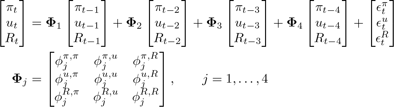
Thus, in Stock and Watson (2001), the reduced-form VAR involves three equations: current unemployment as a function of past values of unemployment, inflation, and the interest rate; current inflation as a function of past values of inflation, unemployment, and the interest rate; and current interest rate as a function of past values of inflation, unemployment, and the interest rate. Stock and Watson (2001) consider traditional Granger causality tests in each equation where the null hypothesis is $H_0{ }^{*}:\theta =0,$ where θ is the appropriate subset of vec $({\Phi }_{\text{1}},{\Phi }_{\text{2}}, . . . ,{\Phi }_{\text{p}}).$ For example, unemployment does not Granger-cause inflation if

${\varphi }_{{ }_{\text{1}}}^{{ }^{\pi ,\text{u}}}={\varphi }_{\text{2}}^{\pi ,\text{u}}={\varphi }_{\text{3}}^{\pi ,\text{u}}={\varphi }_{\text{4}}^{\pi ,\text{u}}=0$

If unemployment does not Granger-cause inflation, then lagged values of unemployment are not useful for predicting inflation.

3 The gcrobustvar command

3.1 Syntax

The gcrobustvar command implements the VAR-based Granger causality robust test. The general syntax of the gcrobustvar command is

gcrobustvar depvarlist, pos(#, #)[ nocons horizon(#) lags(numlist) trimming(level) ]

depvarlist is a list of dependent variables, that is, all the variables in y _t in the notation in (6).

3.2 Options

pos(#, #) is a numeric list (that is, numlist in Stata) including two integers indicating the positions of the targeted dependent variable and restricted regressor, respectively. For example, if we are testing whether the second variable, y _{2 ,t}, Granger-causes the first variable, y _{1 ,t}, in the presence of instabilities, then we assign the numeric list as pos(1,2), where the integer 1 refers to the position of the targeted dependent variable in the VAR (that is, y _{1 ,t} in this example) and the integer 2 refers to the position of the targeted restricted regressor in the VAR (that is, y _{2 ,t} in this example). pos() is required.

nocons suppresses the constant term. The default regression includes the constant term.

horizon(#) specifies the targeted horizon, that is, h in the notation in (4). The default refers to a reduced-form VAR assuming homoskedastic idiosyncratic shocks. When horizon(h) (h ≥ 0) is specified, the command assumes heteroskedastic and serially correlated idiosyncratic shocks and chooses the truncation lag used in the estimation of the long run variance. The truncation lag is automatically determined using Newey and West (1994) optimal lag-selection algorithm. Note that horizon(0) refers to a reduced-form VAR assuming heteroskedastic and serially correlated idiosyncratic shocks, and horizon(h) (h > 0) refers to the (h + 1)-step-ahead forecasting model; see (4). For example, in a one-year-ahead VAR–LP forecasting model with quarterly data, horizon(3) should be specified.

lags(numlist) specifies the lags included in the VAR. The default is lags(1 2). This option takes a numlist and not simply an integer for the maximum lag. For example, lags(2) would include only the second lag in the model, whereas lags(1 2) would include both the first and second lags in the model. The shorthand to indicate the range follows numlist in Stata.

trimming(level) is the trimming parameter. As is standard in the structural break literature, the possible break dates are usually trimmed to exclude the beginning and end of the sample period. If we specify trimming(µ), the range where we search for instabilities is set to be [µT, (1 − µ)T ], where T is the number of total periods. The default is trimming(0.15), which is recommended in the structural break literature and commonly used in practice.

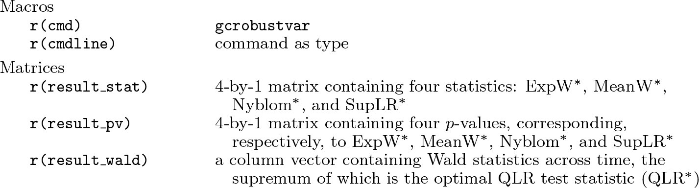
3.3 Stored results

gcrobustvar stores the following in r():

3.4 Empirical example of practical implementation in Stata

In what follows, we illustrate how to use the gcrobustvar command to implement the robust Granger causality test in Stata. The data (GCdata.xlsx, provided with the article files) include quarterly U.S. data on the rate of price inflation $({\pi }_{\text{t}}),$ the unemployment rate (u _t), and the interest rate (R _t, specifically, the federal funds rate) from 1959:I–2000:IV. These are the same variables used in Stock and Watson (2001). Inflation is computed as ${\pi }_{\text{t}}=\text{ 4}00\times \text{ln}(P_{\text{t}}/P_{\text{t}-\text{1}}),$ where P _t is the chain-weighted gross domestic product price index. Quarterly data on u _t and R _t are quarterly averages of their monthly values.

Consider the inflation equation in (3):

$\begin{array}{l}{\pi }_{\text{t}}=c_{\text{t}}^{\pi }+ {\Phi }_{{ }_{\text{t}}}^{\pi ,\pi }(L){\pi }_{\text{t}}+ {\Phi }_{{ }_{\text{t}}}^{\pi ,u}(L)u_{\text{t}}+ {\Phi }_{{ }_{\text{t}}}^{\pi ,R}(L)R_{\text{t}}+{\epsilon }_{{ }_{\text{t}}}^{\pi }\\ \text{where }\hspace{0.17em}\hspace{0.17em}\hspace{0.17em}\hspace{0.17em}{\Phi }_{\text{t}}^{·,·}(L) ={\phi }_{\text{1},\text{t}}^{·,·}L+{\phi }_{2,\text{t}}^{·,·}{L}^{\text{2}}+{\phi }_{3,\text{t}}^{·,·}{L}^{\text{3}}+{\phi }_{4,\text{t}}^{·,·}{L}^{\text{4}}\end{array}$

Suppose we are interested in testing whether unemployment (u) Granger-causes inflation (π), and we want the test to be robust to instabilities over time. That is, we want to test whether the coefficients of lagged values of unemployment (u) are zero across time:

$H_0:{\phi }_{\text{j},\text{t}}^{\pi ,\text{u}}=0\hspace{0.17em}\hspace{0.17em}\hspace{0.17em}\hspace{0.17em}\hspace{0.17em}\hspace{0.17em}\hspace{0.17em}\hspace{0.17em}\hspace{0.17em}\hspace{0.17em}\forall j=\text{ 1},\text{2},\text{3},\text{4}\hspace{0.17em}\hspace{0.17em}\hspace{0.17em}\hspace{0.17em}\hspace{0.17em}\forall t=\text{ 1},\text{2}. . . T$

Implementing the Granger causality tests in the presence of instabilities

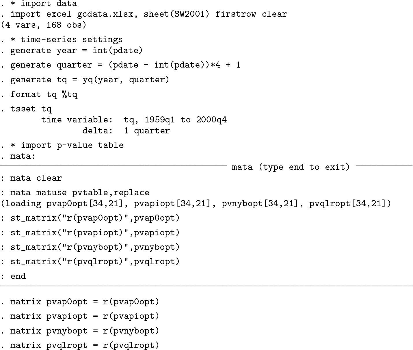
The following scripts implement the Granger causality robust test. We first import the data, claim the data to be time series, and import the p-value tables needed for the tests:

Then, we run the Granger causality robust test using the gcrobustvar command. When we run the gcrobustvar command, important information (variables, lags, etc.) will be displayed:

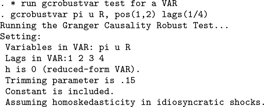
The results are displayed in the following script. The gcrobustvar command provides the four optimal test statistics (ExpW^*, MeanW^*, Nyblom^*, QLR^*) and their corresponding p-values:

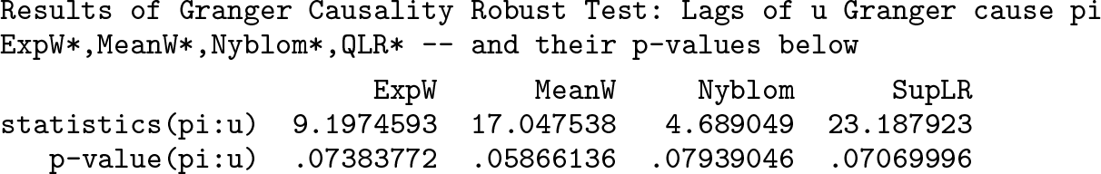
Here is how we get all the inputs of the gcrobustvar command. depvarlist lists the variables included in the VAR, that is, π, u, and R in this order. Because we are testing whether lags of the second variable, u _t, Granger-cause the first variable, π _t, in the presence of instabilities, we assign the positions pos(1,2). As for the options, we include the constant term and include four lags, that is, lags(1/4), as in Stock and Watson (2001). In addition, we assume homoskedasticity and choose the standard trimming parameter 0.15.

Here is how to interpret the results. Let’s take the ExpW^* statistics as an example. The value of ExpW^* is 9.20, and the p-value is 0.07. Thus, the test rejects the null hypothesis that unemployment (u) does not Granger-cause inflation (π) for all t at the 10% significance level.

4 Comparison with the traditional Granger causality test

In this section, we compare the robust Granger causality tests with the traditional Granger causality test in the three-variable VAR model in Stock and Watson (2001). The VAR includes a constant term and four lags and assumes homoskedastic idiosyncratic shocks.

Table 1 reports the p-values of the traditional Granger causality Wald statistics. The results show that π Granger-causes R, u Granger-causes both π and R, and R Granger-causes u at the 5% significance level.

Table 2 reports the p-values of the robust Granger causality test statistics (for ExpW^*, MeanW^*, Nyblom^*, and QLR^*, respectively). We are testing whether the restricted regressor Granger-causes the dependent variable in the presence of instabilities. For example, if we consider the dependent variable π and the restricted regressor R, we are testing whether R Granger-causes π in a way robust to instabilities across time, that is, whether the coefficients of lags of R are constant and equal to zero over time. The p-value of the ExpW^* statistics in panel A in table 2 is 0.01, so the test does reject the null at the 5% significance level. Hence, R does Granger-cause π.

Comparing tables 1 and 2, we find the empirical conclusions differ if a researcher uses the Granger causality robust test instead of the traditional Granger causality test. In fact, R does not Granger-cause π at the 5% significance level in the traditional Granger causality test, but R does Granger-cause π at the 5% significance level in the Granger causality robust test according to the ExpW^*, Nyblom^*, and SupLR^* test statistics. Hence, there is empirical evidence that lagged values of R can predict π, but the predictive ability shows up only sporadically over time, which is the reason why the traditional Granger causality test does not detect it.

Table 1.

Traditional reduced-form VAR-based Granger causality tests

Restricted regressors	Dependent variable
	π	u	R
π	0.00	0.25	0.00
u	0.01	0.00	0.00
R	0.22	0.00	0.00

NOTE: This table reports p-values of the Wald statistics of the traditional Granger causality test. h = 0 (that is, the reduced-form VAR model), lags = (1, 2, 3, 4), assuming homoskedastic idiosyncratic shocks.

Table 2.

Robust Granger causality tests in the reduced-form VAR

Panel A—ExpW*
Restricted regressors	Dependent variable
	π	u	R
π	0.00	0.20	0.00
u	0.07	0.00	0.00
R	0.01	0.00	0.00

Panel B—MeanW*
Restricted regressors	Dependent variable
	π	u	R
π	0.00	0.44	0.00
u	0.06	0.00	0.00
R	0.20	0.01	0.00

Panel C—Nyblom*
Restricted regressors	Dependent variable
	π	u	R
π	0.00	0.22	0.00
u	0.08	0.00	0.00
R	0.03	0.02	0.00

Panel D—QLR*
Restricted regressors	Dependent variable
	π	u	R
π	0.00	0.08	0.00
u	0.07	0.00	0.00
R	0.00	0.00	0.00

NOTE: This table reports p-values of the statistics of the Granger causality robust test. h = 0 (that is, the reduced-form VAR model), lags = (1, 2, 3, 4), the trimming parameter µ = 0.15, assuming homoskedastic idiosyncratic shocks.

gcrobustvar also returns a graph showing the whole sequence of the Wald statistics across time, which gives more information on when the Granger causality occurs. In fact, the optimal QLR^* is the supremum of the sequence of Wald statistics testing whether the parameters are zero at each point in time against the alternative that the parameters change at a given break date at time tq. Figure 1 plots the sequence of the Wald statistics over the possible break dates, reported on the x axis. Consider as an example the test of whether unemployment (u) Granger-causes inflation (π); figure 1 documents the whole sequence of the Wald statistics testing whether unemployment (u) Granger-causes inflation (π). The sequence of the Wald statistic (depicted by a continuous line in figure 1) is above the 10% critical value line (depicted by the dashed lines) around 1970q1 and 1980q1. The figure is saved as gcrobustvar_pi_u.

Figure 1.

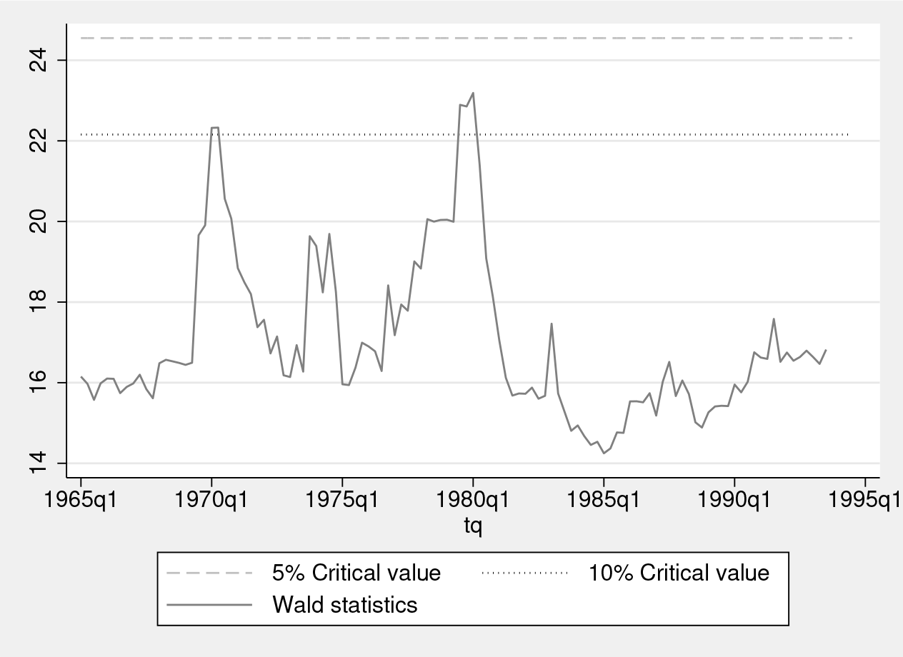
Wald statistics testing whether unemployment (u) Granger-causes inflation (π) against the alternative of a break in Granger causality at time tq (reported on the x axis)

5 Robust Granger causality tests in LP

Section 4 considers the reduced-form VAR assuming homoskedastic idiosyncratic shocks. In this section, we extend the VAR analysis to Jord`a’s (2005) LP by implementing the direct multistep VAR–LP forecasting model in (6) and assuming heteroskedastic and serially correlated idiosyncratic errors. Allowing for heteroskedasticity and serial corre-lation is important when the researcher extends the VAR analysis to LP, where the error terms in (6) can be both heteroskedastic and serially correlated.

We consider the one-year-ahead VAR–LP forecasting model with a constant term and four lags. The setting is similar to section 4 except that we specify h = 3 and relax the homoskedasticity assumption.

The following is the command to implement the robust Granger causality test to investigate whether the coefficients on R _{t − 1} , R _{t − 2} , R _{t − 3} , R _{t − 4} are zero across time in the one-year-ahead VAR–LP forecasting model in the equation where the dependent variable is ${\pi }_{\text{t}+\text{3}}.$ To test other coefficients, we implement the command similarly, except for adjusting the input of pos(#, #).

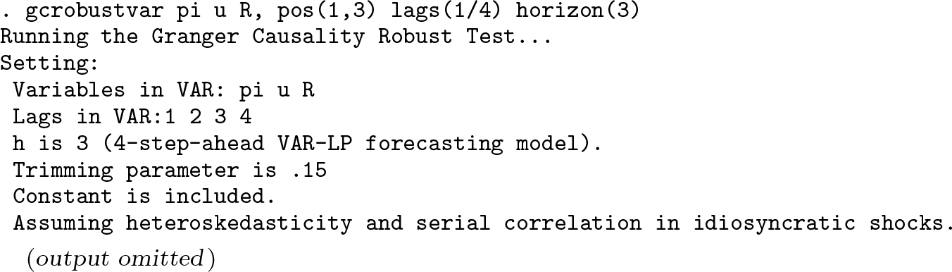
Table 3 reports the p-values of the robust Granger causality test statistics (the ExpW^*, MeanW^*, Nyblom^* and QLR^* statistics, respectively). The results show that lags of inflation (π) can significantly forecast the one-year-ahead unemployment (u) and interest rate (R), lags of unemployment can significantly forecast the one-yearahead inflation and interest rate, and lags of interest rate can significantly forecast the one-year-ahead inflation and unemployment.

Table 3.

Robust Granger causality tests in the direct multistep VAR-LP forecasting model

Panel B—MeanW*
Restricted regressors	Dependent variable
	π	u	R
π	0.00	0.00	0.00
u	0.00	0.00	0.00
R	0.00	0.00	0.00

Panel C—Nyblom*
Restricted regressors	Dependent variable
	π	u	R
π	0.00	0.00	0.00
u	0.00	0.00	0.00
R	0.00	0.00	0.00

Panel D—QLR*
Restricted regressors	Dependent variable
	π	u	R
π	0.00	0.00	0.00
u	0.00	0.00	0.00
R	0.00	0.00	0.00

NOTE: This table reports p-values of the statistics of the Granger causality robust test. h = 3 (that is, the one-year-ahead VAR–LP forecasting model), lags = (1, 2, 3, 4), the trimming parameter µ = 0.15, assuming heteroskedastic and serially correlated idiosyncratic shocks.

7 Programs and supplemental materials

Supplemental Material, st0581 - Vector autoregressive-based Granger causality test in the presence of instabilities

Supplemental Material, st0581 for Vector autoregressive-based Granger causality test in the presence of instabilities by Barbara Rossi and Yiru Wang in The Stata Journal