Sage Journals: Discover world-class research

Abstract

In this article, we introduce a new community-contributed command called xtbunitroot, which implements the panel-data unit-root tests developed by Karavias and Tzavalis (2014, Computational Statistics and Data Analysis 76: 391–407). These tests allow for one or two structural breaks in deterministic components of the series and can be seen as panel-data counterparts of the tests by Zivot and Andrews (1992, Journal of Business and Economic Statistics 10: 251–270) and Lumsdaine and Papell (1997, Review of Economics and Statistics 79: 212–218). The dates of the breaks can be known or unknown. The tests allow for intercepts and linear trends, nonnormal errors, and cross-section heteroskedasticity and dependence. They have power against homogeneous and heterogeneous alternatives and can be applied to panels with small or large time-series dimensions.

Keywords

st0687 xtbunitroot panel data unit root structural break banking COVID-19

1 Introduction

A fundamental property of time-series data is stationarity. If a time series is stationary, then all the standard tools of statistical analysis can be applied; the series can be used in regression models, its mean and variance estimated, and its future forecasted. Frequently, though, time series are nonstationary, or unit-root processes as they are called, and in this case their statistical analysis is different. If nonstationarity is not accounted for, many problems arise for inference and prediction, the most notable of which is that of spurious regression; see, for example, Granger and Newbold (1974). Spurious regression leads to high R² and statistically significant coefficients, when in fact there might be no relationship between the series of interest. Therefore, determining whether a series is stationary should be one of the first steps in any time-series and panel-data (which consist of multiple time series) analysis. Unit-root tests are statistical hypothesis tests used to infer whether a series is a unit root or a stationary process; see, for example, Dickey and Fuller (1979).

In a seminal article, Perron (1989) demonstrated that structural breaks can adversely impact the behavior of unit-root tests. Structural breaks are shocks that are exogenous to the model but have a lasting effect because they change the model parameters. Structural breaks occur when a system is hit by large-scale phenomena; in economics, for example, such events include wars, policy changes, a pandemic like COVID-19, or a financial crisis. These shocks can make stationary series look as if they are nonstationary and therefore mislead the unit-root tests to accept the null hypothesis of nonstationarity when it is not true. To deal with this problem, Perron (1989) proposed new unitroot tests that allow for a structural break in the constant and trend of the series. Perron’s approach, however, assumed that the date of the structural break is known to the researcher. Zivot and Andrews (1992) and Banerjee, Lumsdaine, and Stock (1992) extended Perron (1989) by allowing the date of the break to be endogenously determined by the data, and Lumsdaine and Papell (1997) further extended Zivot and Andrews (1992) to the case of two structural breaks at unknown dates.

Structural breaks can affect panel (longitudinal) data unit-root tests in the same way. In response, Karavias and Tzavalis (2014) proposed panel-data unit-root tests that allow for structural breaks in the intercepts of the series or in both the intercepts and linear trends. The break dates are assumed to be common for all series, but the magnitude of the break can differ across series. The null hypothesis is the same as in Zivot and Andrews (1992) and Lumsdaine and Papell (1997); under the null, the panel series are assumed to constitute unit-root processes without breaks, while under the alternative, they are stationary around breaking means or breaking means and trends.

The Karavias and Tzavalis (2014) tests are widely applicable and possess some unique optimality properties, as has been shown in Karavias and Tzavalis (2017, 2019). In terms of applicability, they can be used in both small- and large-T settings, where T is the number of time-series observations. They allow for multiple common breaks, and the dates of the breaks can be known or unknown. In the latter case, they can be endogenously determined from the data. The errors can be nonnormal and have cross-sectional heteroskedasticity and dependence. Finally, the autoregressive coefficients under the alternative can be homogeneous or heterogeneous, which means that either they can be the same for all units or they can differ between units. In terms of their optimality properties, the tests are invariant under the null to the initial condition, which means that no assumptions on the first observations are necessary, as is the case in other fixed-T tests. Furthermore, the tests are invariant to the coefficients of the deterministic components, and are powerful in the presence of linear trends.

This article introduces xtbunitroot, a new community-contributed command that implements the panel-data unit-root tests of Karavias and Tzavalis (2014). The command includes the options of one or two breaks at known or unknown dates. This is the first command that allows for panel unit-root tests with structural breaks, and therefore it is a complement to the official xtunitroot command and the community-contributed multipurt (Eberhardt 2011), xtfisher (Merryman 2005), and pescadf (Lewandowski 2007) commands.

The breaks can affect the intercepts only or the intercepts and the linear trends of the series. If the dates of the breaks are unknown, then a bootstrap procedure described in Karavias and Tzavalis (2019) is used to derive the critical value and the p-value of the test. Other options include the allowance of cross-section heteroskedasticity, crosssection dependence as in O’Connell (1998), and normal errors. Unbalanced panels are also supported.

The xtbunitroot command is applied to examine stationarity in four fundamental bank balance sheet variables frequently used in the banking literature: returns on assets, returns on equity, total assets, and noninterest income. Their stationarity properties affect model building and economic evaluation; see, for example, Kripfganz and Sarafidis (2021) and Delis and Karavias (2015), and in panel forecasting, see, for example, Liu, Moon, and Schorfheide (2020). We examine a sample of 500 randomly selected U.S. banks for the period 2018Q3 to 2020Q4. This period contains the shock of the COVID- 19 pandemic and the lockdown, which could have caused a structural break in the series. We find that returns on assets, returns on equity, and noninterest income are stationary, but total assets are nonstationary.

The remainder of the article is organized as follows. In section 2, we present the panel unit-root tests as developed by Karavias and Tzavalis (2014) and their extension to two breaks along the lines of Karavias and Tzavalis (2019). This section also provides some Monte Carlo simulations on the behavior of the tests with two breaks. The simulations have been done using the xtbunitroot command. Section 3 describes the syntax of xtbunitroot. Section 4 illustrates the command by analyzing the four banking variables. Section 5 concludes the article.

2 Panel unit-root tests with structural breaks

2.1 One break

For panels with N cross-section units, T time-series observations, and one common break, Karavias and Tzavalis (2014) give two models. The first model can be used to test the null hypothesis of a random walk against the alternative hypothesis of a stationary series with a break in the intercepts (means) of the series,

\begin{array}{l} H_{0} : & y_{i, t} = y_{i, t - 1} + u_{i, t} \\ H_{1} : & y_{i, t} = φ y_{i, t - 1} + (1 - φ) \{a_{1, i} I (t \leq b) + a_{2, i} I (t > b)\} + u_{i, t} \end{array}

where i = 1,…, N and t = 1,…, T. In the above model, φ is the autoregressive parameter, and a₁ _,i and a₂ _,i are the fixed effects before and after the break, which happens on date b. The notation I(·) denotes the indicator function.

The second model tests the null hypothesis of a random walk with drift against the alternative of a trend-stationary panel process with a break in the intercepts and linear trends at time b:

H_{0} : y_{i, t} = y_{i, t - 1} + β_{i} + u_{i, t}

and

\begin{array}{l} H_{1} : y_{i, t} = φ y_{i, t - 1} + φ \{β_{1, i} I (t \leq b) + β_{2, i} I (t > b)\} \\ + (1 - φ) \{a_{1, i} I (t \leq b) + a_{2, i} I (t > b)\} \\ + (1 - φ) \{β_{1, i} t I (t \leq b) + β_{2, i} t I (t > b)\} + u_{i, t} \end{array}

In the above formulation, β_i is the drift under the null hypothesis, while β₁ _,i and β₂ _,i are the trend coefficients under the alternative hypothesis.

We will henceforth denote by M1 the model with intercepts (1) and by M2 the model with both intercepts and trends (2). For M1, the break is allowed to be in I₁ = {1, 2,…, T − 1}, and for M2 the break is allowed to be in I₂ = {2,…, T − 2}.¹

The alternative hypothesis is homogeneous across different individuals, but Karavias and Tzavalis (2016) have shown that the test has power against heterogeneous alternatives as well, when φ_i ≠ φ_j and φ_i, φ_j < 1 for i, j = 1,…, N and i ≠ j. Furthermore, Juodis, Karavias, and Sarafidis (2021) argue that pooled estimators can lead to power gains as opposed to mean-group-type estimators like those of Im, Pesaran, and Shin (2003).

Karavias and Tzavalis (2014) propose estimating the autoregressive parameter φ with the following pooled least-squares estimator,

\hat{φ} = {(\sum_{i = 1}^{N} y_{i, - 1}^{'} Q_{m}^{b} y_{i, - 1})}^{- 1} (\sum_{i = 1}^{N} y_{i, - 1}^{'} Q_{m}^{b} y_{i}), m = {M 1, M 2}

where y _i = (y_i, ₁ ,…, y_i,T )′ and y _i, ₋ ₁ = (y_i, ₀ ,…, y_i,T ₋ ₁)′ are T × 1 vectors. The orthogonal projection matrix $Q_{m}^{b}$ is defined as $Q_{m}^{b} = I_{T} - X_{m}^{b} {(X_{m}^{b'} X_{m}^{b})}^{- 1} X_{m}^{b'}$ , where I _T is the T × T identity matrix and $X_{M 1}^{b} = (e_{1}, e_{2})$ and $X_{M 2}^{b} = (e_{1}, e_{2}, τ_{1}, τ_{2})$ are T × 2 and T × 4 matrices, respectively, where

e_{1, t} = \{\begin{array}{l} 1 & if t \leq b \\ 0 & elsewhere \end{array}, e_{2, t} = \{\begin{array}{l} 1 & if t > b \\ 0 & elsewhere \end{array}

And

τ_{1, t} = \{\begin{array}{l} t & if t \leq b \\ 0 & elsewhere \end{array}, τ_{2, t} = \{\begin{array}{l} t & if t > b \\ 0 & elsewhere \end{array}

The superscripts b in $Q_{m}^{b}$ and $X_{m}^{b}$ denote dependence on the break date.

The estimator $\hat{φ}$ is asymptotically inconsistent; therefore, it must be modified. If the date of the break b is known, the following statistic is asymptotically normally distributed as N → ∞,

Z (b) = \sqrt{N} {\{C^{b} (k_{u}, σ_{u}^{2})\}}^{- 1 / 2} (\hat{φ} - B^{b} - 1) \overset{L}{\to} N (0, 1)

where B^b is the bias correction and C^b is the variance of the bias-corrected (modified) estimator. The parameters k_u and $σ_{u}^{2}$ are error moments to be estimated, but if the errors are normally distributed, they are removed from C^b , which becomes a simple function of the break date and the number of time-series observations. Normality also removes any nuisance parameters related to cross-section heteroskedasticity. The assumptions for the above result are mild, with the strongest being that there is no residual serial correlation in the errors u_i,t .

To deal with cross-sectional dependence in error terms, one popular approach is demeaning the series across i by subtracting the cross-sectional averages for all t before conducting the test (see, for example, O’Connell [1998]),

{\tilde{y}}_{i, t} = y_{i, t} - {\bar{y}}_{t}

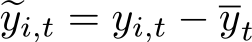
where

{\bar{y}}_{t} = \frac{1}{N} \sum_{i = 1}^{N} y_{i, t}

If the date of the break is unknown, Karavias and Tzavalis (2014) follow Zivot and Andrews (1992) and propose the following statistic to test for unit roots:

\min Z = \min_{b \in I_{m}} Z (b) f o r m = \{M_{1}, M_{2}\}

The limiting distribution of this statistic is shown to depend on the time dimension T. Following Karavias and Tzavalis (2019), the xtbunitroot command implements a bootstrap algorithm to derive the critical values and p-values of minZ. The asymptotic distribution is valid for T fixed and N → ∞. The xtbunitroot command also reports the date with the most evidence against the null hypothesis $\hat{b} = \arg \min_{b \in I_{m}} Z (b)$ . Notice, however, that the break date estimator is not consistent. For consistent break date estimation in small or large T, one may use the xtbreak command of Ditzen, Karavias, and Westerlund (2021) (see also Karavias, Narayan, and Westerlund [Forthcoming]).

The xtbunitroot command supports unbalanced panels. In this case, the missing values in the formulas are zeroed out because this method maximizes the power of tests; see, for example, Karavias, Tzavalis, and Zhang (2022).

2.2 Extension to two-break case

The alternative hypotheses in M₁ and M₂ allow for two breaks. In this case, (1) and (2) become

\begin{array}{l} H_{1} : y_{i, t} = φ y_{i, t - 1} \\ + (1 - φ) \{a_{1, i} I (t \leq b_{1}) + a_{2, i} I (b_{1} < t \leq b_{2}) + a_{3, i} I (t > b_{2})\} + u_{i, t} \end{array}

and

\begin{array}{l} H_{1} : y_{i, t} = φ y_{i, t - 1} + φ \{β_{1, i} I (t \leq b_{1}) + β_{2, i} I (b_{1} < t \leq b_{2}) + β_{3, i} I (t > b_{2})\} \\ + (1 - φ) \{a_{1, i} I (t \leq b_{1}) + a_{2, i} I (b_{1} < t \leq b_{2}) + a_{3, i} I (t > b_{2})\} \\ + (1 - φ) \{β_{1, i} t I (t \leq b_{1}) + β_{2, i} t I (b_{1} < t \leq b_{2}) + β_{3, i} t I (t > b_{2})\} + u_{i, t} \end{array}

The pooled least-squares estimator is based on the $Q_{m}^{b_{1}, b_{2}}$ orthogonal projection matrix, where $Q_{m}^{b_{1}, b_{2}} = I_{T} - X_{m}^{b_{1}, b_{2}} {(X_{m}^{b_{1}, b_{2} /} X_{m}^{b_{1}, b_{2}})}^{- 1} X_{m}^{b_{1}, b_{2}'}$ and where $X_{M 1}^{b_{1}, b_{2}} = (e_{1}, e_{2}, e_{3})$ and $X_{M 2}^{b_{1}, b_{2}} = (e_{1}, e_{2}, e_{3}, τ_{1}, τ_{2}, τ_{3})$ are T × 3 and T × 6 matrices, respectively, with

e_{1, t} = \{\begin{array}{l} 1 & if t \leq b_{1} \\ 0 & elsewhere \end{array}, e_{2, t} = \{\begin{array}{l} 1 & if b_{1} < t \leq b_{2} \\ 0 & elsewhere \end{array}, e_{3, t} = \{\begin{array}{l} 1 & if t > b_{2} \\ 0 & elsewhere \end{array}

The vector τ_t is defined as

τ_{1, t} = \{\begin{array}{l} t & if t \leq b_{1} \\ 0 & elsewhere \end{array}, τ_{2, t} = \{\begin{array}{l} t & if b_{1} < t \leq b_{2} \\ 0 & elsewhere \end{array}, τ_{3, t} = \{\begin{array}{l} t & if t > b_{2} \\ 0 & elsewhere \end{array}

The distributions of the test statistics are as before; Z(b₁ , b₂) is standard normal when b₁ and b₂ are known, and

\min Z = \min_{b_{1}, b_{2} \in I_{m}} Z (b_{1}, b_{2}) for m = \{M_{1}, M_{2}\}

can be used when the dates of the breaks are unknown. Its limiting distribution can be calculated using the bootstrap. Notice that b₁ and b₂ cannot be in two consecutive dates for M2, which is the same situation as in a single time series; see, for example, Lumsdaine and Papell (1997). The xtbunitroot command implements a bootstrap algorithm to derive the critical values and p-values. This asymptotic distribution is valid for T fixed and N → ∞, and the combination of dates with the most evidence against the null hypothesis ${{\hat{b}}_{1}, {\hat{b}}_{2}} = {argmin}_{b_{1}, b_{2} \in I_{m}} Z (b)$ is reported.

To provide some evidence on the behavior of the test statistic with two breaks, we conduct a small Monte Carlo experiment. Consider the data-generation process in (1) and (2) under the null and (3) and (4) under the alternative. We assume that the error term u_i,t ∼ independent and identically distributed N(0, 1). The panel-data series y_i,t is generated with autoregressive coefficient ϕ = 1 to investigate the size at 5% significance level and ϕ = {0.90, 0.95} to investigate the power of the test. As we set ϕ very close to 1, it will be hard to reject the null under H1 : ϕ < 1. The initial values y_i, ₀ are generated as y_i, ₀ ∼ independent and identically distributed N(0, 1). For the M1 and M2 models, we generate the intercept and trend coefficients as follows: a₁_,i ∼ U(−0.5, 0), a₂_,i ∼ U(0, 0.5), and a₃_,i ∼ U(0.5, 1). The slope coefficients for the linear trends are generated as β₁_,i ∼ U(0, 0.025), β₂_,i ∼ U(0.025, 0.05), and β₃_,i ∼ U(0.05, 0.075). These parameter choices follow Karavias and Tzavalis (2014) and are made to make it harder to reject the null H₀ : φ = 1. We set break dates to the following fractions of the sample, λ₁ = 0.25, λ₂ = 0.75. The number of bootstrap replications is set to 100, which is the default in xtbunitroot.

The results of the exercise appear in table 1. We can see that for both known and unknown breaks, the size of the tests is always very close to its nominal 5% level, and the power is satisfactory and increasing with both N and T.

Table 1.

Size and power of the tests for two known and unknown breaks

Panel A: Known breaks
ϕ = 1					ϕ = 0.95			ϕ = 0.90
	(N, T)	10	25	50	10	25	50	10	25	50
M1	25	0.060	0.057	0.071	0.180	0.359	0.719	0.311	0.684	0.990
	50	0.055	0.062	0.053	0.226	0.566	0.915	0.441	0.918	1.000
	100	0.050	0.054	0.061	0.355	0.809	0.996	0.687	0.995	1.000
M2	25	0.056	0.059	0.070	0.062	0.087	0.184	0.077	0.170	0.607
	50	0.052	0.051	0.060	0.059	0.093	0.258	0.077	0.240	0.840
	100	0.055	0.061	0.057	0.064	0.117	0.384	0.095	0.375	0.985

Panel B: Unknown breaks
ϕ = 1					ϕ = 0.95			ϕ = 0.90
	(N, T)	10	15	25	10	15	25	10	15	25
M1	25	0.030	0.030	0.030	0.070	0.250	0.410	0.270	0.580	0.770
	50	0.020	0.050	0.070	0.300	0.440	0.700	0.580	0.810	0.970
	100	0.020	0.070	0.040	0.400	0.720	0.930	0.810	0.990	1.000
M2	25	0.080	0.050	0.060	0.080	0.070	0.060	0.100	0.100	0.130
	50	0.060	0.080	0.050	0.070	0.060	0.050	0.070	0.100	0.080
	100	0.060	0.040	0.010	0.050	0.040	0.040	0.050	0.080	0.200

Notes: The reported values are rejection probabilities. For ϕ = 1, the reported rejection rates give the size of the test, while for ϕ < 1, they give the power of the test. The M1 model includes intercepts, while the M2 model includes both intercepts and linear trends. The dates of the breaks are b₁ = ⌊0.25T⌋, b₂ = ⌊0.75T⌋.

3 The xtbunitroot command

3.1 Syntax

xtbunitroot varname [if ] [in ] [, trend known( #₁ [#₂ ] ) unknown( #₃ [#₄ ] ) normal csd het nobootstrap showindex level( #) seed( #) ]

where varname is the variable to be tested for nonstationarity. You must xtset your data before using xtbunitroot. If no option is specified, the default will be the model with a single break in the intercepts, at an unknown date: xtbunitroot varname, unknown(1 100). varname can contain time-series operators.

3.2 Options

trend specifies that the deterministic component of the model include individual intercepts (means) and individual linear trends. The common breaks affect both intercepts and trends. Breaks in consecutive dates are not allowed in this model. In this model, the breaks can be in dates from 3 to T − 2, while in the model with intercepts, the breaks can take place from 2 up to T − 1.

known( #₁ [#₂ ] ) specifies the number and places of breaks. This option implements the case when the dates of the breaks are known. The #₁ input specifies the location of the first break, and the [#₂ ]input specifies the location of the second break. If only one break is assumed, known( #₁ ) can be used. The inputs should be in terms of time ordering (from 1 to T), instead of using dates, that is, 1995 or 2020. The break dates should be in order. For example, known(5) means the break occurs in period 5, and known(3 7) means the first break occurs in period 3 and the second break occurs in period 7.

unknown( #₃ [#₄ ] ) specifies the number of breaks and the number of bootstrap replications. This option is used when the dates of the breaks are unknown to the researcher. The number of bootstrap replications, [#₄ ], can be omitted. The option unknown(2) states that there are two unknown breaks and the critical and p-values will be calculated based on the default number of bootstrap replications, which is set to 100.

normal specifies that the errors be normally distributed.

csd subtracts the cross-section averages for each time period and applies the tests in the demeaned series.

het specifies that the errors be cross-sectionally heteroskedastic. If both het and normal are specified, the results will be the same as in the case that only normal is used, because if the errors are normal, then heteroskedastic variances drop out.

nobootstrap prevents the command from running the bootstrap. The bootstrap is necessary for calculating critical values and p-values for the test when the dates of the breaks are unknown. However, if the dataset is very large, then the bootstrap can be time consuming. This option stops the bootstrap but returns the minZ statistic and the estimated break dates. The minZ statistic can then be compared with the approximate critical values that appear in table 1 of Karavias and Tzavalis (2014), which is reported in the command output. This option can be used only with the option normal because the available critical values are for normally distributed errors.

showindex specifies that the estimated break date be reported as a time index. For example, an estimated break point at the 9th observation will be reported as 9 instead of 2021q4.

level(#) specifies the level of the test used. The default is level(5), and all integers between 1 and 99 are applicable. For example, level(10) sets the level of the one-sided null hypothesis to 10%.

seed(#) specifies the seed used in the bootstrap process for the case of unknown breaks. The default is seed(123). Seed is important for reproducing bootstrap-based results.

3.3 Stored results

xtbunitroot stores the following in r() :

4 Example

4.1 Unit-root tests for bank balance sheet variables

Unit-root processes were originally important for macroeconomic variables. However, as Holtz-Eakin, Newey, and Rosen (1988) argue, such dynamic relationships can appear in other economic variables for which long time series may not be available. In this case, the panel dimension of the data can be used for inference.

In this section, we focus on bank balance sheet variables taken from the call reports of the Federal Deposit Insurance Corporation. This is a very popular dataset; see, for example, Kripfganz and Sarafidis (2021) and Juodis, Karavias, and Sarafidis (2021) for some recent applications. However, while stationarity of the bank balance sheet variables is frequently assumed, it is almost never tested. The contribution of this section is to examine the stationarity of four variables of interest, namely, returns on assets, returns on equity, total assets, and noninterest income. The returns on assets (roa) are defined as net income after taxes and extraordinary items and is given as a percent of average total assets. The returns on equity (roe) are defined as net income over average total equity; total assets (tassets) are the year-to-date average of total assets; and noninterest income (nii) is defined as income derived from bank services and sources other than interest bearing assets, over average total assets.

We collect data for a random sample of 500 banks from the third quarter of 2018 to the fourth quarter of 2020. This period includes the COVID-19 pandemic, which may have caused breaks in the intercepts and trends of the series. The short dimension of the data is chosen so that our sample of banks does not suffer from survivorship bias. The data are publicly available, and they have been downloaded from the Federal Deposit Insurance Corporation website.²

In the following, we perform panel unit-root tests allowing for structural breaks in the aforementioned variables. We assume that our sample is large enough so that the idiosyncratic errors u_i,t are normally distributed. The errors can be cross-sectionally heteroskedastic, but under the normality assumption, the tests are invariant to heteroskedasticity. Finally, we assume error cross-section dependence, caused possibly by the monetary policy rate.

We start the analysis with the roa series. First, we assume that the date of the break is known to be the first quarter of 2020. Second, we allow the break to be unknown and determined from the data. In the latter case, the critical values are taken using 100 bootstrap samples, which is the default. The results are given below:

The output above indicates that the Z(b) statistic is equal to −15.521, which is far less than the critical value of −1.645; therefore, we can reject the null hypothesis of nonstationarity. The break under the alternative takes place in observation 7, which corresponds to the first quarter of 2020. The output also reports the result “the null is rejected”, which is the outcome at the 5% significance level. The following output presents the results for roa, when the date of the break is unknown.

We can see from the above output that the $\min Z$ statistic is equal to −25.162, which is much smaller than the bootstrap critical value of 8.555; therefore, we once more reject the null hypothesis. The p-value is also reported and implies that the null hypothesis is rejected at the 1% significance level. The date with the most evidence against the null is observation 6, which corresponds to the fourth quarter of 2019, although this estimator is not expected to provide a consistent estimate of the break date, as mentioned earlier.

For the remaining three variables, we will implement the tests being agnostic about the date of the break. For tassets and nii, we also include linear trends.

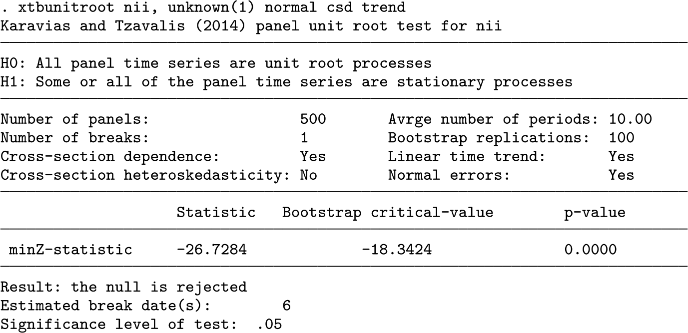
As we can see from the above outputs, roe and nii are stationary, while tassets is not. When the null hypothesis is not rejected at the 5% level, the output does not report the break date; however, this date can be recovered from r(break1). In smaller datasets, one may wish to employ higher levels of significance using the level() option. For tassets, the date with the most evidence against the null is the first quarter of 2019; however, the p-value is high, and we cannot reject the null hypothesis.

5 Concluding remarks

This article introduced a new community-contributed command, xtbunitroot, that implements the panel-data unit-root tests with structural breaks, developed by Karavias and Tzavalis (2014). This is the first command that allows for panel unit-root tests with structural breaks; it allows for one or two breaks under an alternative that can be known or unknown. It also allows for linear trends, cross-sectional heteroskedasticity and dependence, and nonnormal errors. The xtbunitroot command was applied to four bank balance sheet variables, and it was found that returns on assets, returns on equity, and noninterest income are stationary variables, but total assets are nonstationary.

6 Programs and supplemental materials

Supplemental Material, sj-zip-1-stj-10.1177_1536867X221124541 - Panel unit-root tests with structural breaks

Supplemental Material, sj-zip-1-stj-10.1177_1536867X221124541 for Panel unit-root tests with structural breaks by Pengyu Chen, Yiannis Karavias and Elias Tzavalis in The Stata Journal

Footnotes

Notes

6 Programs and supplemental materials

To install a snapshot of the corresponding software files as they existed at the time of publication of this article, type

References

Banerjee

Lumsdaine

R. L.

Stock

J. H.

1992. Recursive and sequential tests of the unit-root and trend-break hypotheses: Theory and international evidence. Journal of Business and Economic Statistics 10: 271–287. https://doi.org/10.2307/1391542.

Delis

M. D.

Karavias

2015. Optimal versus realized bank credit risk and monetary policy. Journal of Financial Stability 16: 13–30. https://doi.org/10.1016/j.jfs.2014.11.004.

Dickey

D. A.

Fuller

W. A.

1979. Distribution of the estimators for autoregressive time series with a unit root. Journal of the American Statistical Association 74: 427–431. https://doi.org/10.2307/2286348.

Ditzen

Karavias

Westerlund

2021. Testing and estimating structural breaks in time series and panel data in Stata. ArXiv Working Paper No. arXiv:2110.14550. https://arxiv.org/abs/2110.14550.

Eberhardt

. 2011. multipurt: Stata module to run 1st and 2nd generation panel unit root tests for multiple variables and lags. Statistical Software Components S457239, Department of Economics, Boston College. https://ideas.repec.org/c/boc/bocode/s457239.html.

Granger

C. W. J.

Newbold

1974. Spurious regressions in econometrics. Journal of Econometrics 2: 111–120. https://doi.org/10.1016/0304-4076(74)90034-7.

Holtz-Eakin

Newey

Rosen

H. S.

1988. Estimating vector autoregressions with panel data. Econometrica 56: 1371–1395. https://doi.org/10.2307/1913103.

K. S.

Pesaran

M. H.

Shin

2003. Testing for unit roots in heterogeneous panels. Journal of Econometrics 115: 53–74. https://doi.org/10.1016/S0304-4076(03)00092-7.

Juodis

Karavias

Sarafidis

2021. A homogeneous approach to testing for Granger non-causality in heterogeneous panels. Empirical Economics 60: 93–112. https://doi.org/10.1007/s00181-020-01970-9.

10.

Karavias

Narayan

P. K.

Westerlund

Forthcoming. Structural breaks in interactive effects panels and the stock market reaction to COVID-19. Journal of Business and Economic Statistics. https://doi.org/10.1080/07350015.2022.2053690.

11.

Karavias

Tzavalis

2014. Testing for unit roots in short panels allowing for a structural break. Computational Statistics and Data Analysis 76: 391–407. https://doi.org/10.1016/j.csda.2012.10.014.

12.

Karavias

Tzavalis

2016. Local power of fixed‐T panel unit root tests with serially correlated errors and incidental trends. Journal of Time Series Analysis 37: 222–239. https://doi.org/10.1111/jtsa.12144.

13.

Karavias

Tzavalis

2017. Local power of panel unit root tests allowing for structural breaks. Econometric Reviews 36: 1123–1156. https://doi.org/10.1080/07474938.2015.1059722.

14.

Karavias

Tzavalis

2019. Generalized fixed‐T panel unit root tests. Scandinavian Journal of Statistics 46: 1227–1251. https://doi.org/10.1111/sjos.12392.

15.

Karavias

Tzavalis

Zhang

2022. Missing values in panel data unit root tests. Econometrics 10: 12. https://doi.org/10.3390/econometrics10010012.

16.

Kripfganz

Sarafidis

2021. Instrumental-variable estimation of large-T paneldata models with common factors. Stata Journal 21: 659–686. https://doi.org/10.1177/1536867X211045558.

17.

Lewandowski

. 2007. pescadf: Stata module to perform Pesaran’s CADF panel unit root test in presence of cross section dependence. Statistical Software Components S456732, Department of Economics, Boston College. https://ideas.repec.org/c/boc/bocode/s456732.html.

18.

Liu

Moon

H. R.

Schorfheide

2020. Forecasting with dynamic panel data models. Econometrica 88: 171–201. https://doi.org/10.3982/ECTA14952.

19.

Lumsdaine

R. L.

Papell

D. H.

1997. Multiple trend breaks and the unit-root hypothesis. Review of Economics and Statistics 79: 212–218. https://doi.org/10.1162/003465397556791.

20.

Merryman

. 2005. xtfisher: Stata module to compute Fisher type unit root test for panel data. Statistical Software Components S448201, Department of Economics, Boston College. https://ideas.repec.org/c/boc/bocode/s448201.html.

21.

O’Connell

P. G. J

. 1998. The overvaluation of purchasing power parity. Journal of International Economics 44: 1–19. https://doi.org/10.1016/S0022-1996(97)00017-2.

22.

Perron

1989. The great crash, the oil price shock, and the unit root hypothesis. Econometrica 57: 1361–1401. https://doi.org/10.2307/1913712.

23.

Zivot

Andrews

D. W. K.

1992. Further evidence on the Great Crash, the oil price shock, and the unit-root hypothesis. Journal of Business and Economic Statistics 10: 251–270. https://doi.org/10.2307/1391541.