Testing and estimating structural breaks in time series and panel data in Stata

Abstract

Identifying structural change is a crucial step when analyzing time series and panel data. The longer the time span, the higher the likelihood that the model parameters have changed because of major disruptive events such as the 2007–2008 financial crisis and the 2020 COVID-19 outbreak. Detecting the existence of breaks and dating them is therefore necessary for not only estimation but also understanding drivers of change and their effect on relationships. In this article, we introduce a new community-contributed command called xtbreak, which provides researchers with a complete toolbox for analyzing multiple structural breaks in time series and panel data. xtbreak can detect the existence of breaks, determine their number and location, and provide break-date confidence intervals. We use xtbreak in examples to explore changes in the relationship between COVID-19 cases and deaths in the US using both aggregate and state-level data and in the relationship between approval ratings and consumer confidence using a panel of eight countries.

1 Introduction

In economics and elsewhere, linear relationships between dependent and explanatory variables are at the core of interest. To investigate such relationships, researchers collect observations over time for one or more cross-sectional units such as firms, individuals, or countries and subsequently use them in estimating the coefficients of regression models. A key assumption here is that the coefficients do not change over time. This assumption is unlikely to hold, especially for longer periods of time, because of major disruptive events such as financial crises. Parameter instability can have a detrimental impact on estimation and inference and can lead to costly errors in decision making. The times in which the parameters change are called “change points” in the statistics literature and “structural breaks” in economics. Because both terms are synonymous to each other, we will use the latter term or just “breaks”.

In this article, we propose a new community-contributed command called xtbreak. ¹ The package implements the methods developed by Bai and Perron (1998) for pure time series and Ditzen, Karavias, and Westerlund (2025) for panel data. ²

xtbreak provides researchers with a complete toolbox for analyzing multiple structural breaks in time series and panel data. It can detect and date an unknown number of breaks at unknown break dates. The toolbox is based on asymptotically valid tests for the presence of breaks, a consistent break-date estimator, and a break date confidence interval with correct asymptotic coverage. In fact, xtbreak includes three tests: 1) a test of no structural breaks against the alternative of a specific number of breaks, 2) a test of the null hypothesis of no structural breaks against the alternative of an unknown number of structural breaks, and 3) a test of the null of s breaks against the alternative of s + 1 breaks. The package also includes an algorithm that uses the last test consecutively to estimate the true number of breaks. The tested break dates can be unknown or user defined, as when researchers have additional information and wish to examine whether there was a break in a specific point in time. Once the presence of breaks has been tested and confirmed, xtbreak estimates the locations of the breaks and provides the associated confidence intervals.

Having many breaks does not translate into heavy computational burden: xtbreak implements an efficient dynamic programming method described in Bai and Perron (2003) that ensures that there are O(T²) computations even with more than two breaks, where T is the number of time-series observations.

xtbreak can deal with models of “pure” or “partial” structural breaks. In a pure structural-breaks model, the coefficients of all explanatory variables change, while in a partial structural-breaks model, only a subset of the coefficients changes.

xtbreak is applicable under very general error conditions. For time-series data, the only requirement is that there are no unit roots in the errors. For panel data, units can be independent or cross-sectionally dependent, where cross-sectional dependence takes an “interactive fixed effects” or “common factor” structure. Regressors can load on the same set of factors as the errors, which means that regressors may be endogenous—although no instrumental variables are necessary. The errors can also be serially correlated and heteroskedastic but not nonstationary.

The works of Bai and Perron (1998) and Ditzen, Karavias, and Westerlund (2025) draw on the economics literature. However, structural breaks also happen in other fields of research, including engineering, epidemiology, climatology, and medicine. xtbreak is therefore widely applicable. To showcase this width, we consider two examples drawn from the areas of epidemiology and political economy. First, we consider the epidemiological relationship between COVID-19 cases and deaths. Using both aggregate country and disaggregated state-level US data, we find evidence of multiple breaks. In particular, we find that an increase in the number of COVID-19 cases led to more deaths in the beginning of the pandemic than in later waves. Second, we examine if there are breaks in the relationship between consumer confidence and the approval ratings of country leaders. Using a panel of eight countries observed over a long period of time, we find that there is great cross-country heterogeneity in terms of the number and locations of breaks.

The remainder of the article is organized as follows: Section 2 presents the model that we will be considering. We focus on the panel case, which in most regards includes the pure time series setup as a special case. Important differences are brought up and discussed. Sections 3, 4, and 5 present the hypothesis tests, the break-date estimation procedure, and the xtbreak command, respectively. Sections 6 and 7 contain the empirical analyses of the COVID-19 and leader approval ratings data, respectively. Section 8 concludes the article.

2 Model discussion

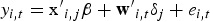
We consider the following model with N units, T periods, and s structural breaks:

$$y_{i,t}={{\mathrm{x}}^{\mathrm{\prime }}}_{i,j}\beta +{{\mathbf{w}}^{\mathrm{\prime }}}_{i,t}{\mathit{\delta }}_j+e_{i,t}$$

(1)

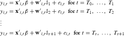
$t=T_{j-1},\dots ,T_j$ and $j=1,\dots ,s+1$ with T₀ = 0 and $T_{s+1}=T$ . Hence, there are s breaks, or s + 1 regimes with regime j covering the observations $T_{j-1},\dots ,T_j$ . To emphasize the break structure, we can write (1) regimewise:

$$\begin{array}{rl}& y_{i,t}={{\mathbf{x}}^{\mathrm{\prime }}}_{i,t}\mathit{\beta }+{{\mathbf{w}}^{\mathrm{\prime }}}_{i,t}{\mathit{\delta }}_1+e_{i,t}\mathrm{for}t=T_0,\dots ,T_1\\ & y_{i,t}={{\mathbf{x}}^{\mathrm{\prime }}}_{i,t}\mathit{\beta }+{{\mathbf{w}}^{\mathrm{\prime }}}_{i,t}{\mathit{\delta }}_2+e_{i,t}\mathrm{for}t=T_1,\dots ,T_2\\ & ⋮\\ & y_{i,t}={{\mathbf{x}}^{\mathrm{\prime }}}_{i,t}\mathit{\beta }+{{\mathbf{w}}^{\mathrm{\prime }}}_{i,t}{\mathit{\delta }}_{s+1}+e_{i,t}\mathrm{for}t=T_s,\dots ,T_{s+1}\end{array}$$

For N = 1, this is a time-series model, while for N > 1, it is a panel-data model. The dependent variable $y_{i,t}$ and the regression error $e_{i,t}$ are scalars, while ${\mathbf{x}}_{i,t}$ and ${\mathbf{w}}_{i,t}$ are $p\times 1$ and $q\times 1$ vectors, respectively, of regressors. The coefficients of the regressors in ${\mathbf{x}}_{i,t}$ are unaffected by the breaks, while those of ${\mathbf{w}}_{i,t}$ are affected by the breaks. It is possible that all independent variables break, in which case ${{\mathbf{x}}^{\mathrm{\prime }}}_{i,t}\mathit{\beta }$ is defined to be zero. In the panel case, the break dates are common for all units. This common assumption is reasonable when the frequency of the data is not high. Let ${\mathcal{T}}_s=\{T_1,\dots ,T_s\}$ be a collection of s break dates such that $T_j=\lfloor {\lambda }_{j}T\rfloor$ , where ${\lambda }_0=0<{\lambda }_1<\cdots <{\lambda }_s<{\lambda }_{s+1}=1$ . By specifying the breaks this way, we ensure that they are distinct from one another and bounded away from the beginning and end of the sample. This is important because we need to be able to fit the model within each regime.

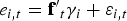
If the data have a panel structure (N > 1), we allow for unobserved heterogeneity in the form of interactive fixed effects:

$$e_{i,t}={{\mathbf{f}}^{\mathrm{\prime }}}_t{\gamma }_i+{\epsilon }_{i,t}$$

(2)

f _t is an m × 1 vector of factors, and ${\gamma }_i$ is a conformable vector of factor loadings. ³ The fact that f_t is common to all cross-sectional units i means that the regression errors can be strongly cross-sectionally correlated. This specification is very general and nests the usual one-way and two-way fixed-effects models as special cases. Both f _t and ${\epsilon }_{i,t}$ may be weakly serially correlated, but they cannot be nonstationary. They can also not be correlated with each other, and ${\epsilon }_{i,t}$ cannot be cross-sectionally correlated. ⁴ This last condition ensures that any cross-sectional dependence in $e_{i,t}$ originates with f _t .

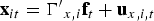
Typically, there is a lot of cross-sectional comovement not only in the regression errors but also in the regressors. To account for this, we assume that ${\mathbf{x}}_{i,t}$ and ${\mathbf{w}}_{i,t}$ are generated as

$${\mathbf{x}}_{it}={{\mathbf{\Gamma }}^{\mathrm{\prime }}}_{x,i}{\mathbf{f}}_t+{\mathbf{u}}_{x,i,t}$$

(3)

$${\mathbf{w}}_{it}={{\mathbf{\Gamma }}^{\mathrm{\prime }}}_{w,i}{\mathbf{f}}_t+{\mathbf{u}}_{x,i,t}$$

(4)

Where ${\mathbf{\Gamma }}_{x,i}$ and ${\mathbf{\Gamma }}_{w,i}$ are $p\times m$ and $q\times m$ matrices, respectively, of factor loadings, while ${\mathbf{u}}_{x,i,t}$ and ${\mathbf{u}}_{w,i,t}$ are $p\times 1$ and $q\times 1$ vectors, respectively, of idiosyncratic errors that are independent of all the other random elements of the model. The model described by (1)–(4) above is the same as the one considered by Ditzen, Karavias, and Westerlund (2025). ⁵

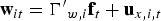
The fact that ${\mathbf{x}}_{i,t}$ and ${\mathbf{w}}_{i,t}$ are allowed to load on the same set of factors as $e_{i,t}$ means that they can be endogenous. This type of endogeneity through unobserved heterogeneity is standard in panel data. Here we are considering interactive fixed effects, but the idea is the same in the fixed-effects case; the effects sitting in errors might also be in the regressors, which means that they have to be removed prior to estimation. In the fixed-effects case, one augments (1) by dummy variables, which is tantamount to transforming the variables into deviations from means. Here a more elaborate augmentation approach is needed, which is to be expected because interactive effects are more general than fixed effects. Had the factors been known, which would be the case if the unobserved heterogeneity were made up of known deterministic terms, for example, we would have estimated

$$y_{i,t}={{\mathbf{x}}^{\mathrm{\prime }}}_{i,t}\beta +{{\mathbf{w}}^{\mathrm{\prime }}}_{i,t}{\delta }_j+{{\mathbf{f}}^{\mathrm{\prime }}}_t{\gamma }_i+{\epsilon }_{i,t}$$

(5)

by ordinary least squares (OLS). This is possible because with f _t as a regressor, the regression error is no longer given by $e_{i,t}$ but by ${\epsilon }_{i,t}$ , which is independent of the regressors. On the other hand, if f _t is not known, then we need a good proxy to use in its stead. ⁶ Ditzen, Karavias, and Westerlund (2025) use ${\overline{\mathbf{x}}}_t=N^{-1}{\sum }_{i=1}^N{\mathbf{x}}_{i,t}$ and ${\overline{\mathbf{w}}}_t=N^{-1}{\sum }_{i=1}^N{\mathbf{w}}_{i,t}$ , and so do we. ⁷ The appropriately augmented version of (1) is therefore given by

$$y_{i,t}={{\mathbf{x}}^{\mathrm{\prime }}}_{i,t}\mathit{\beta }+{{\mathbf{w}}^{\mathrm{\prime }}}_{i,t}{\mathit{\delta }}_j+{{\overline{\mathbf{x}}}^{\mathrm{\prime }}}_t{\mathbf{a}}_i+{{\overline{\mathbf{w}}}^{\mathrm{\prime }}}_t{\mathbf{b}}_{i,j}+\mathrm{error}$$

(6)

Because asymptotically observing the cross-sectional averages is just as good as observing the true factors, the regressors in (6) are asymptotically exogenous. This means that the estimation can be carried out using OLS. This is the same idea as in the common correlated effects (CCE) estimator of (Pesaran 2006), except that here we do not include the cross-sectional average of $y_{i,t}$ as a regressor in (6) (see Karavias, Narayan, and Westerlund [2023] for a discussion). If f _t is neither completely known nor completely unknown, as is usually the case in practice, then the cross-sectional averages will take care of the unknown factors, and the known factors can be added to (6) as additional regressors. ⁸

If N = 1 such that (1) is a time-series model, then by definition, there is no crosssectional variation that we can exploit to estimate unknown factors. Hence, in this case, f_t must be known, so the model to be fit is given by (5), which is then the same as in Bai and Perron (1998).

3 The toolbox

3.1 Hypothesis testing

This section presents the first set of tools, which is necessary for establishing that one or more structural breaks have happened and for determining their number, s. In particular, we consider tests of three hypotheses, labeled 1–3, and a sequential test to determine s. We begin by stating the hypotheses of interest.

H₀: no breaks versus H₁: s breaks, where the number of breaks under H₁, s, is specified by the researcher.

H₀: no breaks versus H₁: 1 ≤ s ≤ s_max breaks, where the maximum number of breaks under H₁, s_max, is specified by the researcher.

H₀: s breaks versus H₁: s + 1 breaks, where s is specified by the researcher.

To test hypotheses 1–3, we use several test statistics. The time-series versions of these tests have appeared in Bai and Perron (1998), while the panel versions have appeared in Ditzen, Karavias, and Westerlund (2025).

Hypothesis 1

If the dates of the breaks are known, we will consider a Chow test for hypothesis 1. Therefore, let us denote by $F({\mathcal{T}}_s)$ the F statistic for testing the null of no breaks versus the alternative of s known breaks at dates ${\mathcal{T}}_s$ , which is based on (5) in the time-series case and on (6) in the panel case. Appropriate critical values can be taken from the F distribution with s numerator degrees of freedom and $N\{T-p-(s+1)q\}-p-(s+1)q$ denominator degrees of freedom.

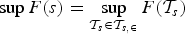
If ${\mathcal{T}}_s$ is unknown, which is most likely the case in practice, then the following supre-mum statistic can be used:

$$supF(s)=\underset{{\mathcal{T}}_s\in {\mathcal{T}}_{s,\in }}{sup}F({\mathcal{T}}_s)$$

Here

$${\mathcal{T}}_{s,\in }=\{(T_1,\dots ,T_s):T_{j+1}-T_j\ge \in T,T_1\ge \in T,T_s\le (1-\in )T\}$$

is the set of permissible break dates, with ∊ being a user-defined trimming parameter. By setting $\in \in (0,1)$ , we ensure that the breaks considered in the test are distinct and bounded away from the sample endpoints as assumed.

Hypothesis 2

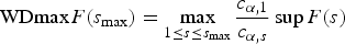
Hypothesis 2 can be tested using the double maximum statistic

$$\mathrm{WDmax}F(s_{max})=\underset{1\le s\le s_{max}}{max}{\displaystyle \frac{c_{\alpha ,1}}{c_{\alpha ,s}}supF(s)}$$

where $c_{\alpha ,s}$ is the critical value of supF(s) at significance level α and s breaks. The weighting by $c_{\alpha ,1}/c_{\alpha ,s}$ here ensures that the marginal p-values of the weighted supremum statistics are all equal. This counterweighs the decrease in the marginal p-value of supF(s) that comes from increasing s and the resulting loss of power when s is large. The test statistic with weights $c_{\alpha ,1}/c_{\alpha ,s}$ for all s is called UDmaxF(s_max).

Hypothesis 3

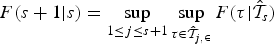
In section 4, we describe a procedure for how to estimate the break dates. Let ${\hat{\mathcal{T}}}_s=\left\{{\hat{T}}_1,\dots ,{\hat{T}}_s\right\}$ be the set of estimated breaks obtained based on that procedure. For the test of hypothesis 3, we use the statistic

$$F(s+1|s)=\underset{1\le j\le s+1}{sup}\underset{\tau \in {\hat{\mathcal{T}}}_{j,\in }}{sup}F(\tau |{\hat{\mathcal{T}}}_s)$$

where ${\hat{\mathcal{T}}}_s$ contains estimates of the s break stipulated under the hull hypothesis, τ is the additional (s + 1)th break under the alternative, and

$${\hat{\mathcal{T}}}_{j,\in }=\{\tau :{\hat{\mathrm{T}}}_{j-1}+({\hat{\mathrm{T}}}_j-{\hat{\mathrm{T}}}_{j-1})\in \le \tau \le {\hat{\mathrm{T}}}_j-({\hat{\mathrm{T}}}_j-{\hat{\mathrm{T}}}_{j-1})\in ,{\hat{\mathrm{T}}}_0=0,{\hat{\mathrm{T}}}_{s+1}=1\}$$

is the set of permissible breaks in between the estimated (j − 1)th and jth breaks. Hence, F(s + 1\vert s) is testing the null of s breaks versus the alternative that there is an additional break somewhere within the regimes stipulated under the null. Finally, $F(\tau |{\hat{\mathcal{T}}}_s)$ is the F statistic based on taking the estimated break dates in ${\hat{\mathcal{T}}}_s$ as given and testing for one additional break at τ.The F(s + 1| s) test can be applied sequentially to estimate the number of breaks. In this case, we start by testing the null of no breaks against the alternative of a single break using F(1| 0). If the null is accepted, we set $\hat{s}=0$ and terminate the procedure. However, if the null is rejected, we estimate the break point, denoted ${\hat{T}}_1$ , and split the sample in two at ${\hat{T}}_1$ . We then test for the presence of a break in each of the two subsamples using F(2\vert 1). If no breaks are found, we set $\hat{s}=1$ and stop, whereas if breaks are detected, we estimate their location and split the sample again. This process continues until the test fails to reject.The asymptotic distributions of the above tests in the pure time-series and panel cases can be found in Bai and Perron (1998) and Ditzen, Karavias, and Westerlund (2025), respectively. Because the distributions are the same, the critical values are the same. xtbreak therefore uses the critical values of Bai and \vert Perron (1998, 2003), which are applicable for ∊ ∊ {0.05, 0.1, 0.15, 0.2, 0.25}. In theory, the validity of the critical values requires T → ∞ in the time-series case and N, T → ∞ with T/N → 0 in the panel case, which in practice means that T should be “large” in both cases and that N should be even larger in the panel case. For some Monte Carlo evidence on the accuracy of these predictions, we refer to Bai and Perron (2003) and Ditzen, Karavias, and Westerlund (2025).

4 Break-date estimation

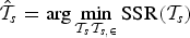
The previous section was focused on testing for the existence of breaks and on determining their number. Now we turn to their location because researchers use break dates to identify the underlying cause of breaks.The standard approach in the literature is to estimate breaks by minimizing the sum of squared residuals. Bai and Perron (1998) and Ditzen, Karavias, and Westerlund (2025) do the same. The break-date estimator included in xtbreak is therefore given by

$${\hat{\mathcal{T}}}_s=\arg \underset{{\mathcal{T}}_s{\mathcal{T}}_{s,\in }}{min}\mathrm{SSR}({\mathcal{T}}_s)$$

where $\mathrm{SSR}({\mathcal{T}}_s)$ is the sum of squared residuals based on s breaks. In the time-series case, the residuals are taken from (5), whereas in the panel case, they are taken from (6). If s is “small”, the minimization can be done by grid search. However, if s is “large”, then grid search, which requires O(T^s) OLS operations, becomes computationally costly and possibly even infeasible. In such cases, the efficient dynamic programming algorithms of Bai and Perron (1998, 2003) and Ditzen, Karavias, and Westerlund (2025), which limit the number of operations to O(T²) for any s, can be used.

Once ${\hat{\mathcal{T}}}_s$ has been obtained, confidence intervals for each estimated break date can be constructed using the formulas given in Bai and Perron (1998) and Ditzen, Karavias, and Westerlund (2025).

5 The xtbreak command

5.1 Syntax

5.1.1 Automatic estimation of number of breaks and break dates

This syntax tests for breaks via hypothesis 2 and estimates the number of breaks and break dates with no prior knowledge on number and location of breaks. Estimation of the number of breaks is based on the sequential test of hypothesis 3.

5.1.2 Testing for known structural breaks

This syntax implements hypothesis 1: testing for breaks if the break dates are known.

5.1.3 Testing for unknown structural breaks

This syntax implements hypotheses 1–3: testing for breaks if the break dates are unknown.The default is hypothesis 3 and option sequential.

5.1.4 Estimation of breakdates

This syntax estimates break dates for a given number of breaks.

5.1.5 Maintenance

xtbreak[, update version] The update option updates xtbreak from GitHub by using net install. The version option displays the version.

5.1.6 Specific options

Options1 are general options and apply to xtbreak in general:

Data must be tsset or xtset (see [TS] tsset or [XT] xtset) before using xtbreak. Time-series data must not include gaps. Panel data can be unbalanced. In this case, observations with missing data will not be included in the regressions. depvar, indepvars, and varlist may contain time-series operators; see [U] 11.4.4 Time-series varlists. xtbreak requires the moremata package (Jann 2005).

5.2 Description of options

xtbreak automatically detects if N = 1 or N >  1. Therefore, the user does not have to specify whether the data have a time series or a panel structure. xtbreak requires the moremata package (Jann 2005).

breakpoints(numlist, index | datelist, fmt(format)) specifies the known break points, which can be set by either the number of corresponding observations or the values of the time identifier. If numlist is used, option index is required. For example, breakpoints(10, index) specifies that one break occurs at the 10th observation as ordered by time. datelist takes a list of dates. For example, breakpoints(2010Q1, fmt(tq)) specifies a break in the first quarter of 2010. The option fmt() specifies the format and is required if datelist is used. The format set in breakpoints() and the time identifier need to be the same.

hypothesis(1| 2| 3) specifies which hypothesis to test. Specify hypothesis(1) for hypothesis 1, hypothesis(2) for hypothesis 2, and hypothesis(3) for hypothesis 3. The default is hypothesis(3) in combination with the option sequential.

showindex shows confidence intervals as the index.

breaks(real) specifies the number of unknown breaks under the alternative. For hypothesis 2, breaks() can include two values. For example, breaks(4 6) tests the null of no breaks against the alternative of 4–6 breaks. If only one value is specified, then the lower bound of the number of breaks under the alternative is set to 1. If hypothesis 3 is tested, then breaks() defines the number of breaks under the alternative. If hypothesis 3 is tested and breaks() is not defined, then option sequential is invoked.

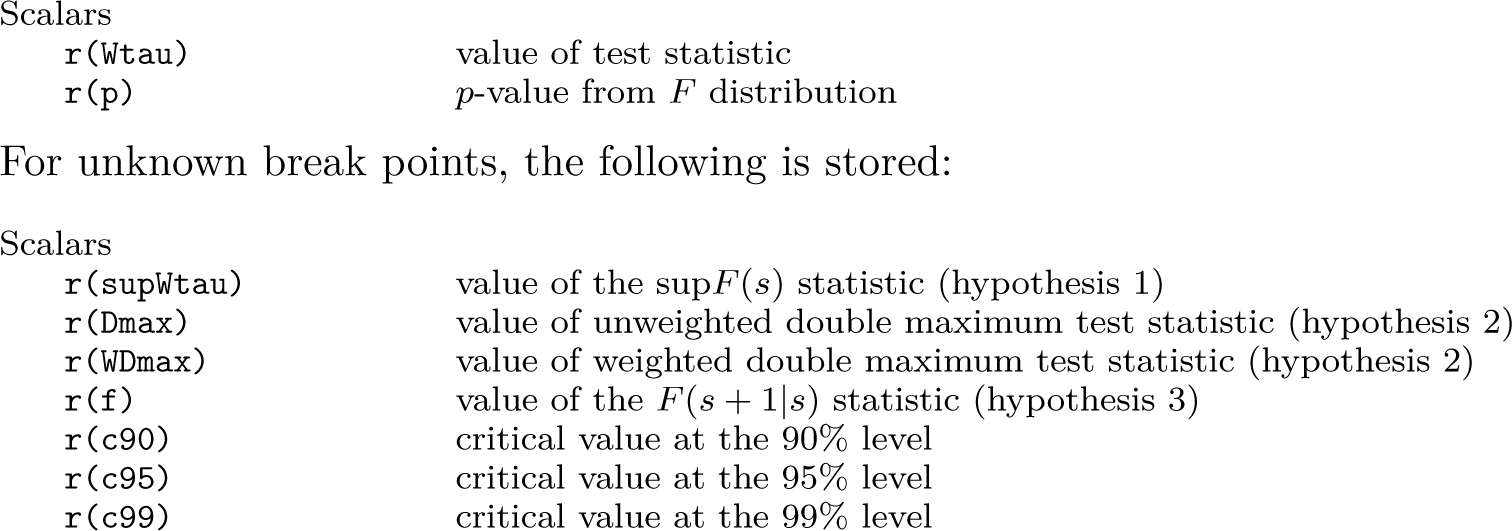
breakconstant adds a break in the constant. The default is no breaks in the constant.

noconstant suppresses the constant.

nobreakvariables(varlist₁) defines variables with no structural breaks. varlist₁ can contain time-series operators.

vce(type) specifies the covariance matrix estimator. The options are ssr (homoskedas-tic errors, the default); hc (heteroskedasticity-robust); hac (heteroskedasticity- and autocorrelation-robust); np (the nonparametric estimator of Pesaran [2006]); and wpn (the fixed-T standard errors of Westerlund, Petrova, and Norkute [2019]).

inverter(type) sets the inverter. type can be speed (invsym()); precision; qr (equivalent to precision; qrinv()); chol (cholinv()); p (pinv()); or lu (luinv()). The choice of inverter has implications on speed and precision. For an overview, see [M-4] Solvers.

python uses Python to calculate segment-specific SSRs to improve speed. This option requires Stata 16 or later, Python, and the following packages: scipy, numpy, pandas, and xarray. Numerical differences in the calculations may occur because of different matrix inverters and precision in Stata and Python. This option can be used only with balanced panels.

trimming(real) specifies the trimming parameter as a percent. The trimming affects the minimal time periods between two breaks. The default is 15% (trimming(0.15)). Critical values are available for 5%, 10%, 15%, 20%, and 25%.

error(real) defines the error margin for the partial break model.

wdmax weighs the double maximum test statistic used for testing hypothesis 2. The default is to not use any weights.

level(#) sets the significance level for critical values for the double maximum test. If a value is chosen for which no critical values exist, xtbreak test will choose the closest level.

sequential specifies the sequential F test to obtain the number of breaks when using hypothesis 3.

breakfixedeffects adds breaks in individual fixed effects. The default is no breaks in fixed effects.

nofixedeffects suppresses individual fixed effects.

csd implements csa(w) csanobreak(x) automatically. For example, the variables in w would enter with breaks, while those in x, specified with the nobreakvariables() option, enter without breaks.

csa(varlist₂) specifies the variables with breaks, which are added as cross-sectional averages. xtbreak automatically calculates the cross-sectional averages.

csanobreak(varlist₃) is the same as csa() but for variables without breaks.

kfactors(varlist₄) specifies that variables in varlist₄ are known factors, or variables in the data that are constant across the cross-sectional dimension. Examples are seasonal dummies or other observed common factors such as asset returns and oil prices. The factors in this list are affected by structural breaks in that their loadings change.

nbkfactors(varlist₅) is same as above, but the factors in varlist₅ are not affected by structural breaks.

noreweigh can be applied only to unbalanced panels. By default, xtbreak reweighs the time-unit-specific errors used in the SSR by weights equal to total number of units in the sample divided by the number of unit observations in that period. Thus, it increases the SSR in segments with missing data. noreweigh avoids reweighting missing data.

skiph2 skips hypothesis 2 (H₀: no break versus H₁: 0 <  s <  s_max breaks) when running xtbreak without the estimate or test option.

cvalue(level) specifies the significance level to be used to estimate the number of breaks using the sequential test. For example, cvalue(0.99) uses the 1% significance level critical values to determine the number of breaks using the sequential test. See level() for further details.

strict enforces strict behavior of the sequential test to determine the number of breaks. The sequential test will stop once F(s + 1| s) is not rejected given a rejection of F(s| s − 1). This option improves speed in large time series but should be used with caution.

maxbreaks(#) limits the maximum number of breaks when using the sequential test.

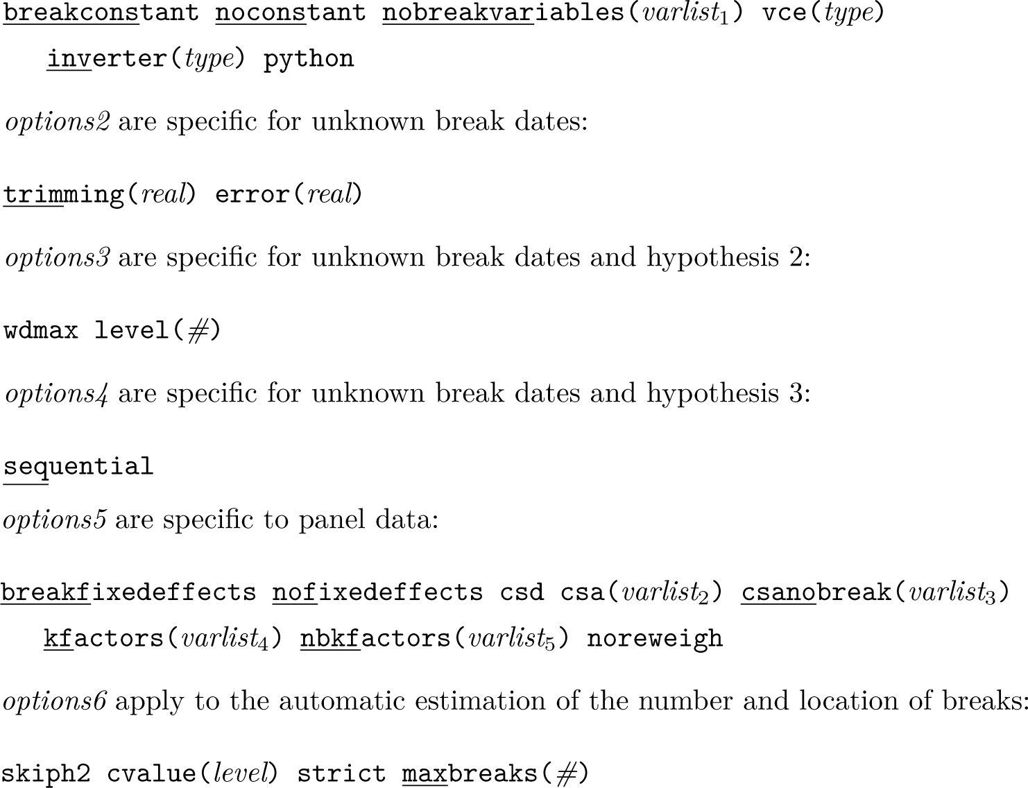
5.3 Stored results

xtbreak estimate stores the following in e():

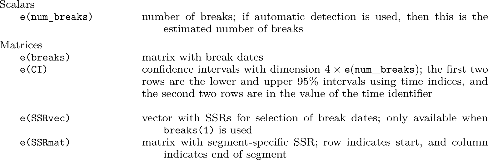
xtbreak test stores the following in r() for known break points:

5.4 Postestimation

The following postestimation commands can be used after xtbreak estimate:

estat indic ator [newvar]

estat indicator creates an indicator variable (1,… , 1, 2,… , 2,… , s + 1,… , s + 1)′ that specifies all break regimes.

estat split [ varlist]

estat split will split a varlist according to the estimated break points and draw a scatterplot of the variable with the break on the x axis and the dependent variable on the y axis, use

estat scatter varname[, twoway_options]

estat indicator creates a new variable of the form (1,… , 1, 2,… , 2,… , s + 1,… , s + 1)′, where the value changes for each break regime. estat split splits the variables defined in varlist according to the break dates and saves the names of the created variables in r(varlist). estat scatter draws a scatterplot with the dependent variable on the y axis and a variable with breaks defined in varname on the x axis.

xtbreak estimate stores information about segment-specific SSRs and the SSRs for different break dates in e(). This information can be used to draw a time-series plot of SSRs across potential break dates with

estat ssr[, tsline_options]

estat ssr is available only after xtbreak estimate y x, breaks(1). tsline_options are any options permitted when using tsline; see [TS] tsline or [G-2] graph twoway tsline.

5.5 On the choice of factors in the panel case

xtbreak is versatile in dealing with common factors, whether they are known (observed) or unknown (unobserved), through the options csd, csa(), csanobreak(), kfactors(), and nbkfactors(). Unknown factors are estimated by the cross-sectional averages specified in csa() and csanobreak() or, alternatively, in csd. Known factors can be dummy variables or other observed variables that do not vary across units and are defined by kfactors() and nbkfactors(). Whenever they are available, known factors should be included because they make it possible to estimate more unknown factors. These factors can be free of breaks, or they can be allowed to break.

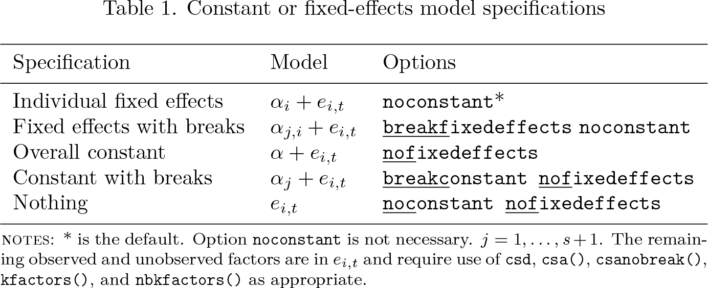
Fixed effects are known factors but are not treated through the kfactors() and nbkfactors() commands so that xtbreak’s command structure can deal with fixed effects similarly to other Stata commands. In particular, one has to specify whether xtbreak should fit a model with or without overall constant or individual fixed effects separately from the factor structure specification. In total, xtbreak supports five different models, which are presented in table 1. The default is a model with fixed effects that are not breaking.

The choice of deterministic model has implications for the analysis of structural breaks. In the overall constant model, the constant is treated as a regular regressor, and we can test and detect breaks in it. In fact, the constant may be the only regressor. In the presence of fixed effects, xtbreak cannot be used without breaking regressors (w_i,t), because it cannot detect or estimate breaks that affect only fixed effects and not the regressors. Once breaking regressors are included, one has the choice to allow for breaking or nonbreaking fixed effects.

5.6 Unbalanced panels

xtbreak can be used with unbalanced panel data. Pure time-series data (N = 1) with gaps are not allowed. For unbalanced panels, there is an appropriate adjustment in the degrees of freedom in the test statistics. It is assumed that missing data are missing completely at random and that all time periods have at least one observation.

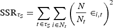
In terms of break-date estimation, xtbreak identifies breaks by minimizing the SSR; see (7). If a value is missing, Stata removes the whole unit-time observation, so the number of summands in the SSR drop, which can lead to estimating break dates away from the true break. To avoid this behavior, xtbreak reweighs the individual time- specific residuals ${\in }_{i,t}$ , and the SSR is calculated as

$${\mathrm{SSR}}_{{\tau }_S}=\sum _{t\in {\tau }_S}{\sum _{i\in N_t}\left({\displaystyle \frac{N}{N_t}{\in }_{i,t}}\right)}^2$$

where N is the number of total units and N_t is the number of units for which data are nonmissing in time period t. N/N_t scales the residuals up when data are missing. The option noreweigh avoids the reweighing by setting N_t = N independently from the number of nonmissing observations.

6 COVID-19 deaths and cases

6.1 Time-series evidence for the whole US

Main results

In this section, we explain the use and options of xtbreak. We want to test whether we can identify structural breaks in the relationship between the number of COVID-19 deaths and cases in the US in 2020 and 2021. This is an interesting topic because COVID- 19’s case fatality rate, which is the number of deaths from COVID-19 over the number of COVID-19 cases, was a key variable of medical and policy interest and consequently was the focus of many studies; see, for example, Mathieu et al. (2020). ⁹ The fatality rate can be time varying because of, for example, countrywide changes in the capability of detecting the virus, lockdowns, population-wide vaccination programs, improvements in treatment and hospital capacity, and the emergence of new strains. All of these events are massive in scale and can cause structural breaks. We use aggregate US weekly time-series data on the number of deaths and new cases from the Centers for Disease Control and Prevention. The dataset is also available on our GitHub page.

We want to fit the model

$$\mathrm{\Delta }{\mathrm{deaths}}_t={\beta }_0+{\delta }_1\mathrm{\Delta }{\mathrm{cases}}_{t-1}+{\delta }_2\mathrm{\Delta }{\mathrm{cases}}_{t-2}+{\delta }_3\mathrm{\Delta }{\mathrm{cases}}_{t-3}+e_t$$

where deaths _t and cases _t are the reported deaths due to COVID-19 in week t and the number of new cases for the entire US in the same week, respectively. We assume that a week lies, on average, between a positive test and a possible death. ¹⁰ The data range from 27 January 2020 (beginning of week 4) to 29 August 2021 (end of week 34). Δ denotes first differencing, which is taken to ensure stationarity. ¹¹ The model is a simplification, although it has been used elsewhere in the literature; see, for example, Silverio et al. (2020) and Fritz (2022).

Table 1.

Constant or fixed-effects model specifications

Specification	Model	Options
Individual fixed effects	${\alpha }_i+e_{i,t}$	noconstant*
Fixed effects with breaks	${\alpha }_{j,i}+e_{i,t}$	breakf ixedeffects noconstant
Overall constant	$\alpha +e_{i,t}$	nof ixedeffects
Constant with breaks	${\alpha }_j+e_{i,t}$	breakc onstant nof ixedeffects
Nothing	$e_{i,t}$	noc onstant nof ixedeffects

Notes: * is the default. Option noconstant is not necessary. j = 1,…, s + 1. The remaining observed and unobserved factors are in $e_{i,t}$ and require use of csd, csa(), csanobreak(), kfactors(), and nbkfactors() as appropriate.

We want to test whether the coefficients δι, δ₂, and δ₃ are subject to structural breaks. There are several reasons to believe that the relationship between the number of new cases and deaths might have changed. At the beginning of the pandemic, the understanding of COVID-19 and the best way to treat the disease were not developed. The numbers were also underreported because of limits in testing capacity and reporting routines. With better testing capacity, reporting routines, and treatments, the relationship is expected to change, especially after the first two waves, because of the knowledge gained. Starting in mid-December 2020, vaccines were introduced. Hence, the relationship between the number of cases and deaths might be expected to have changed again. Therefore, it seems reasonable to expect at least two breaks.

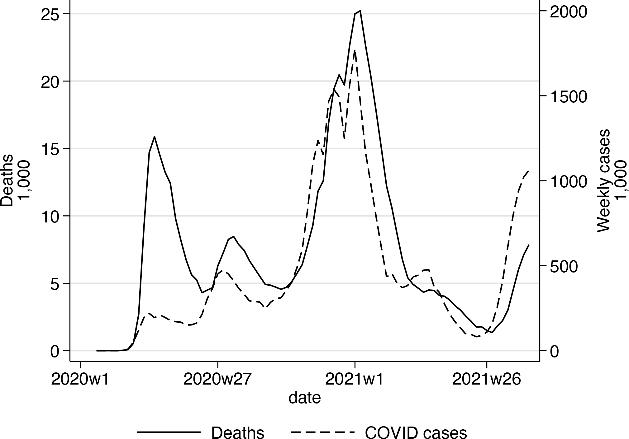
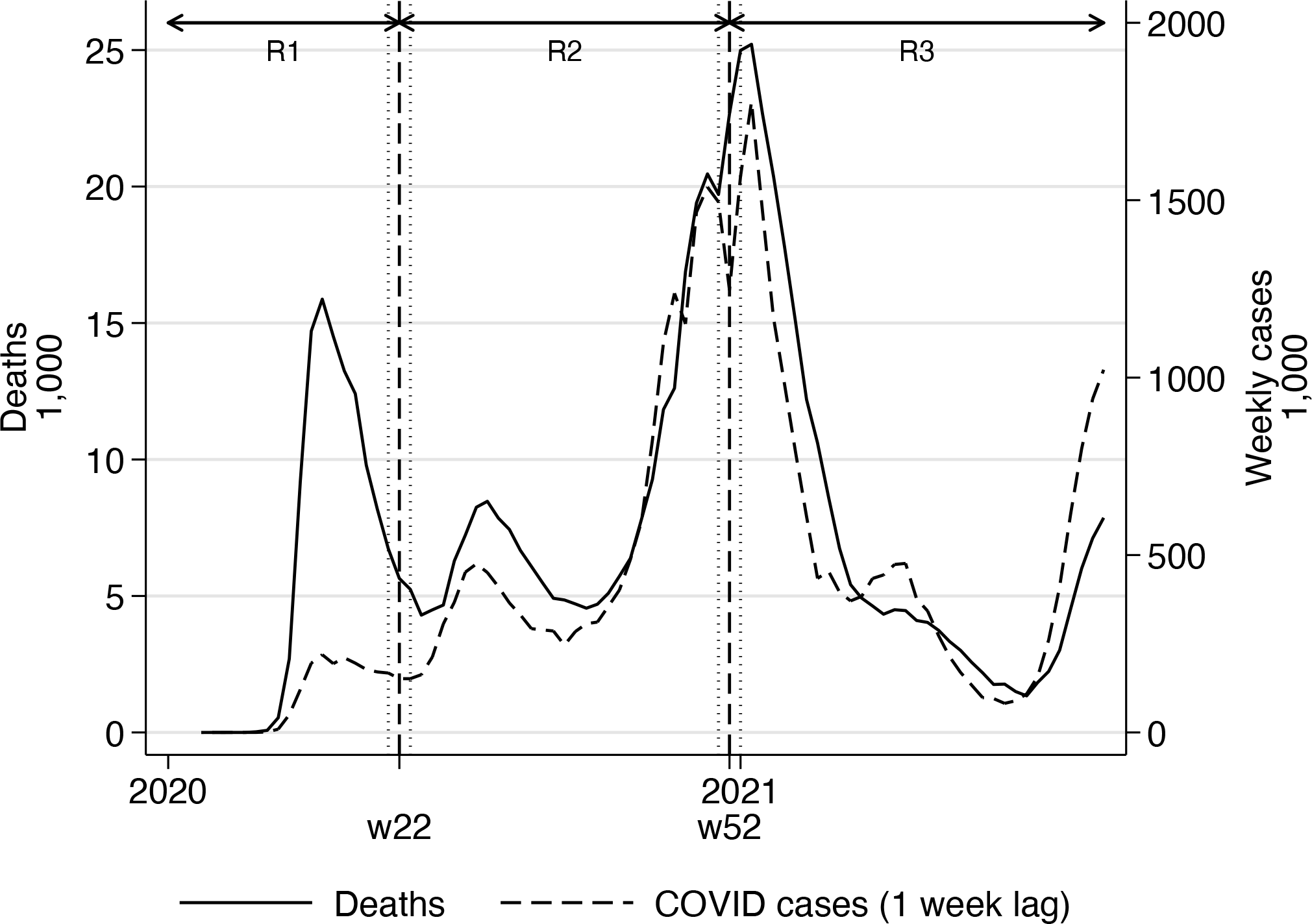
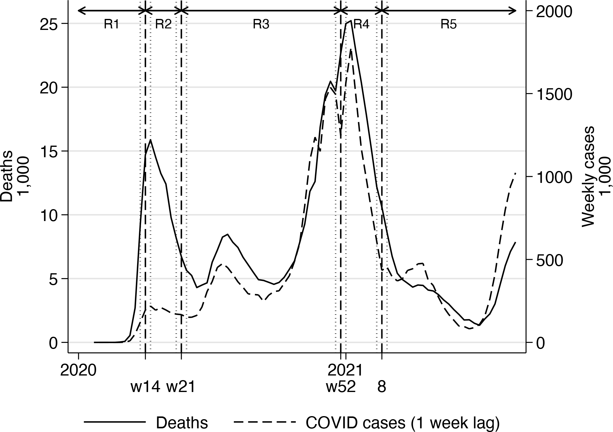
Figure 1 plots the number of deaths and cases over time. Note the striking difference between the number of deaths and cases in the first wave and the number of deaths being many times larger than the number of new cases. This difference is markedly smaller in the second wave, but the number of deaths is still higher. The third wave was the worst in terms of numbers by far, but the number of deaths per new case was much lower than before. From about week 29 in 2020, the number of cases started to pick up again, and so did the number of deaths.

Figure 1.

Plotting COVID-19 deaths and cases over time

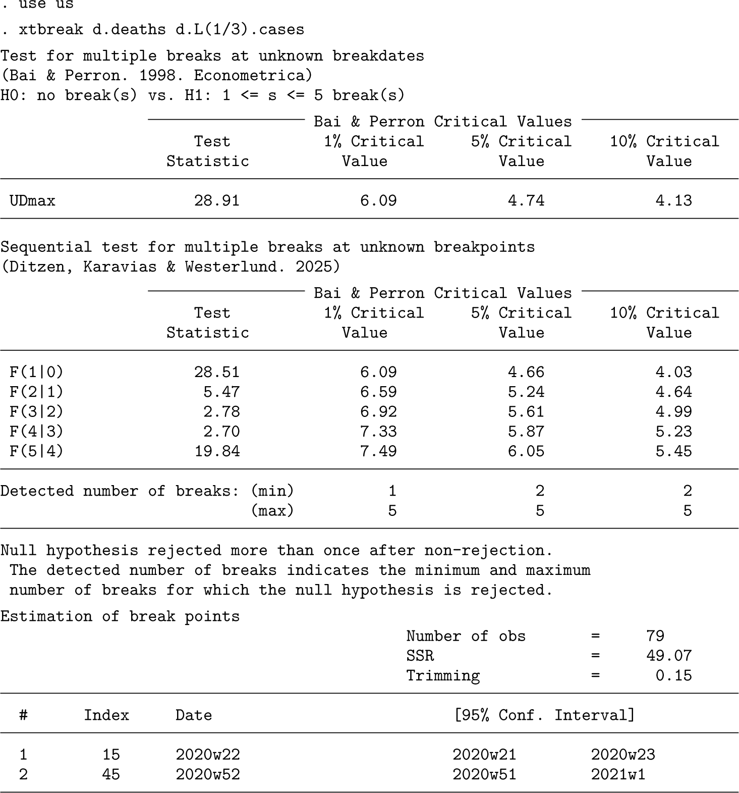
We can use xtbreak without any prior knowledge of the number of breaks or their exact dates. We use the following command line:

xtbreak starts with hypothesis 2; that is, it tests the null hypothesis of no breaks against the alternative of an unknown number of breaks between 1 and s_max breaks. This is the most powerful test, and it does not need knowledge of the number of breaks. The maximum number of breaks is set to s_max = 5. ¹² The value of the UDmax test statistic is 28.91, which is well above the 1% critical value and hence provides evidence for at least 1 and up to 5 breaks. xtbreak then estimates the number of breaks by reporting the test value of hypothesis 3 (H₀: s breaks versus s + 1 breaks) at each step in the sequence and the appropriate critical values for the three basic significance levels. We see that 0 break is rejected in favor of 1 break and that 1 break is rejected in favor of 2 breaks at the 5% significance level, but then, when testing 2 breaks against 3 or more breaks, the test is no longer able to reject. ¹³ Therefore, we conclude that there are 2 breaks. xtbreak then proceeds to report the estimated break dates and the associated confidence intervals. The first break is estimated to week 22 of 2020 (fourth week of May), while the second is estimated at the end of year 2020. The confidence intervals on both breaks span only a couple of weeks, suggesting that the estimates are precise. The confidence interval width is a function of the magnitude of the break, and short confidence intervals hint at larger breaks.

xtbreak saves the values of the break points in e(breaks) and the confidence intervals in e(CI). The matrices contain the index number t ∊ {1,…, T} of both breaks and the confidence interval bounds. We use this information to draw figure 2, in which the estimated break dates and their 95% confidence intervals are plotted in the same graph as the deaths and the lagged number of cases. ¹⁴

Figure 2.

Plotting estimated breaks (dashed lines), 95% confidence intervals (dotted lines), deaths, and lagged cases

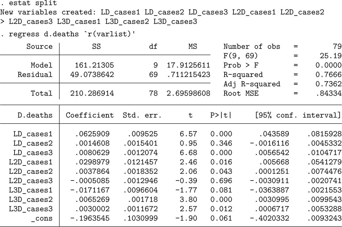
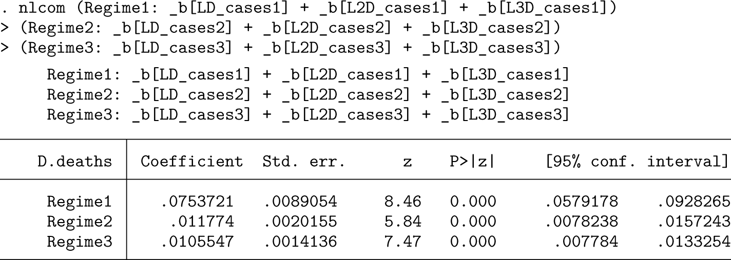
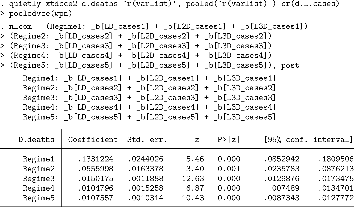
Next we use the estat command of xtbreak to generate new variables for each break regime and run an OLS regression:

The long-run multipliers within each regime are given by ${\delta }_{\mathrm{LR},j}:={\delta }_{1,j}+{\delta }_{2,j}+{\delta }_{3,j}$ for j = 1, 2, 3. They are reported using the nlcom command, which also provides confidence intervals. The ${\delta }_{\mathrm{LR},j}$ capture the total effect in time that an additional 1,000 COVID-19 cases have on deaths in regime j. The estimate for the first regime ${\hat{\delta }}_{\mathrm{LR},j}$ , covering the period from week 4 of 2020 to week 22 of 2020, suggests that for each additional 1,000 cases of COVID-19, 75 people died on average. According to figure 2, the end date of this regime coincides with the end of the first wave. This estimate is quite high, which can be explained by the relatively small number of tests conducted at that time. The estimated effect of the number of cases is much lower in the second regime, which stretches from week 23 of 2020 to week 51 of 2020. Only 12 out of an additional 1,000 infected died. The coefficient of the third regime, lasting from week 1 in 2021 to the end of the sample, is almost the same, where 11 out of an additional 1,000 infected died. This is probably in part due to the vaccination rollout, which began in week 51 of 2020.

Additional results and discussions

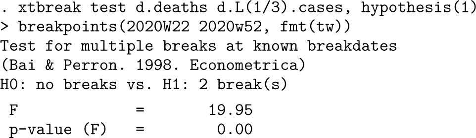
This section is divided in two: 1) additional test results and 2) additional estimation results. The aim is to demonstrate how the command can be used for specific tests and estimations, as opposed to the automatic way used above. We begin by considering additional test results, starting with a test of hypothesis 1. Specifically, we test the null hypothesis of no breaks against the alternative of a break in week 22 in 2020 and another break in week 52 in 2020 using the regular Chow F test. These are the results:

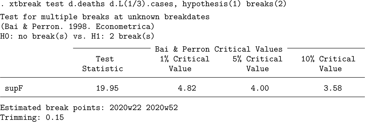
The test value is 19.95, which is way out in the critical region of the F distribution. Therefore, we can comfortably reject the null of no breaks. To test the same hypothesis but with unknown break dates, we specify breaks(2). The results look as follows:

The test value is identical to before, as is the conclusion to reject the null hypothesis, which is to be expected because the given break dates were set to the estimated breaks obtained earlier. The difference is that when the breaks are treated as unknown, the critical values come from a nonstandard distribution because the statistic is the supremum of F tests over all possible break dates because these are determined by the trimming parameter. These critical values are more “honest” than those used for the Chow test because they account for the fact that the breaks are unknown. As a part of the test results, xtbreak reports the estimated break dates used to construct the test, and we can see that they coincide with those obtained earlier.

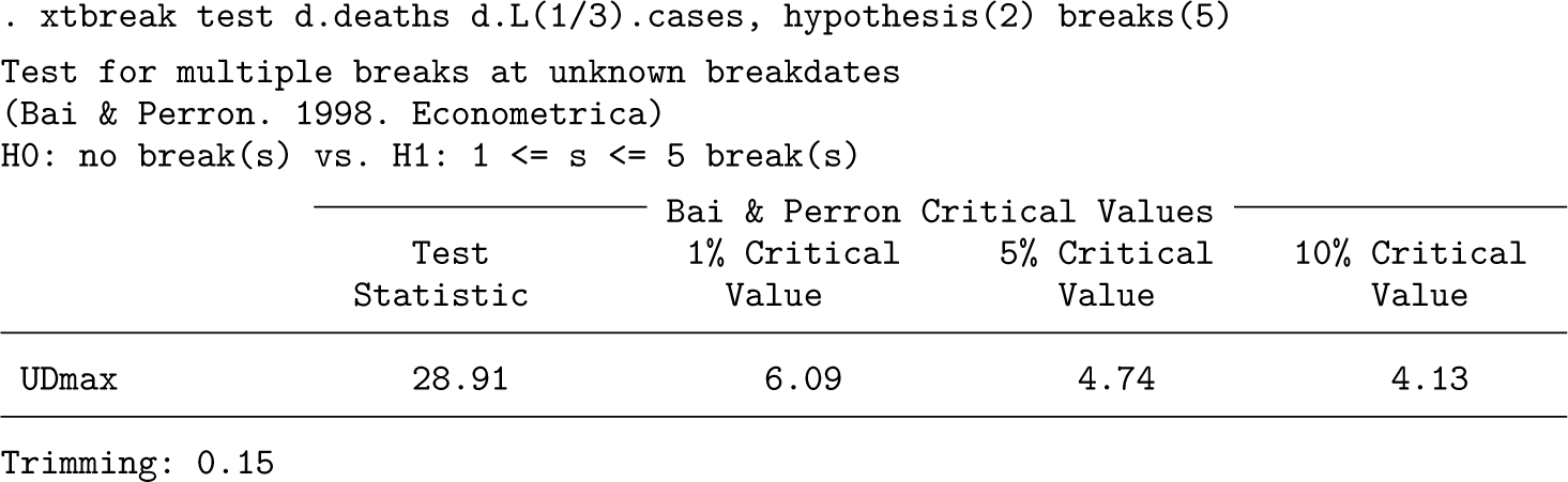
We now test the null of no breaks against the alternative of up to five breaks. This is an example of a test of hypothesis 2, the results of which are presented here below. As expected, the null hypothesis is firmly rejected.

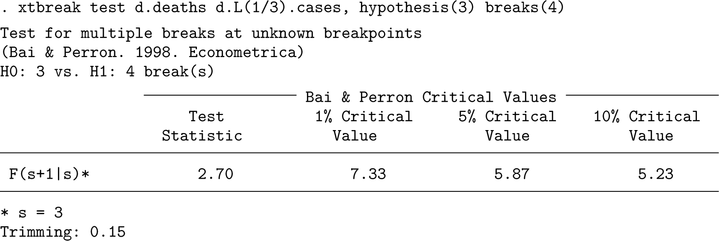
Next we test the null of three breaks against the alternative of four breaks, which is an example of hypothesis 3. We use the options hypothesis(3) and breaks(4) to specify that there are four breaks under the alternative. The results presented below suggest that we are unable to reject the null, which is consistent with the estimated number of breaks.

The option sequential repeats the hypothesis 3 test, sequentially starting from no breaks under the null up to the specified number in breaks. Setting breaks(5) returns the sequential test results reported earlier.

. xtbreak test d.deaths d.L(1/3).cases, hypothesis(3) breaks(5) sequential

As a final test exercise, we consider two changes to the model. We begin by investigating how the above results are affected if we allow for breaks in the constant. To do so, we use the sequential test but add the option breakconstant:

. xtbreak test d.deaths d.L(1/3).cases, breakconstant

To save space, we omit the output, but we briefly describe it; xtbreak finds five breaks. Note also that the options hypothesis(3) and sequential are the defaults, so we have omitted them from the command. We further investigate if the break is only in the constant and not in the number of cases. We keep the option breakconstant and move the variable L.cases to the option nobreakvar(L.cases):

. xtbreak test d.deaths, breakconstant nobreakvar(d.L(1/3).cases)

Now xtbreak detects no breaks at the 5% significance level, meaning that the breaks are driven from changes in the slope coefficients.

We end this section with some comments on the estimation results. The break-date results reported earlier can be obtained using the option xtbreak estimate. The appropriate command line is

. xtbreak estimate d.deaths d.L(1/3).cases, breaks(2)

As an illustration of the fitted regression model, we can draw a scatterplot with different symbols for the observations within each regime. The plot can be created using xtbreak estat:

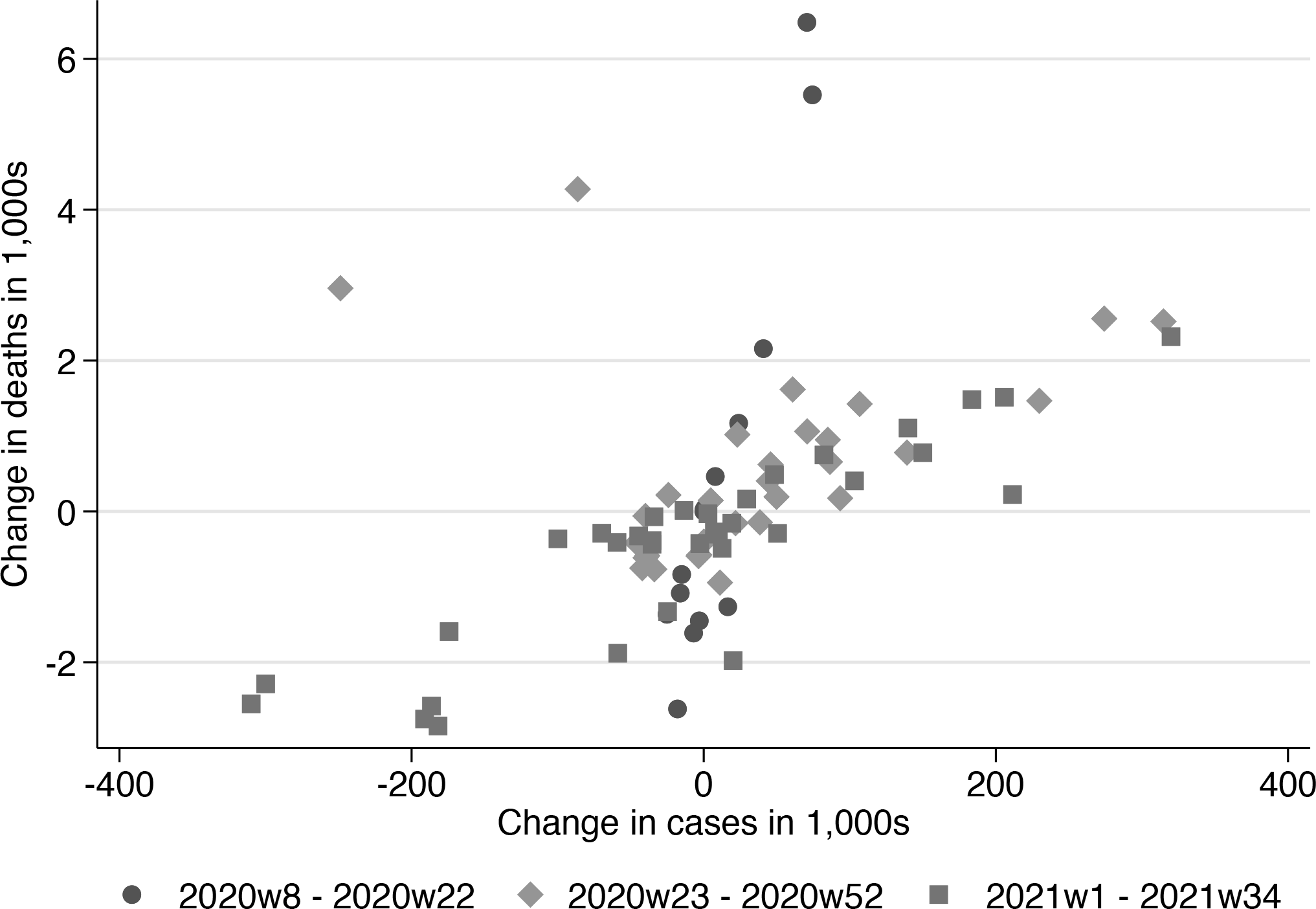
The plot is displayed in figure 3. The different markers represent the observations within each regime, and the location of the observations is indicative of the strength of the estimated linear relationships and of their slopes. The first regime is described by dots that appear in an almost vertical line. The second and third regimes are described by rhombi and squares, respectively, that mostly lie along the 45-degree line. In particular, we see that the slope in the first regime differs quite markedly compared with the other two, which confirms the findings from the OLS regression. twoway_options (see [G-3] twoway_ options) can be passed through. Option autolegend(legend_op-tions) automatically creates the legend labels for each segment. legend_options (see [G-3] legend _options) are further options passed to legend(), as done here to control the placement and number of columns of the legend.

Figure 3.

Scatterplotting lagged cases against deaths by regime

6.2 State-level panel evidence

Main results

In this section, we use the same US data as in the previous section; however, instead of aggregating the data up to the country level, we use data for all 50 US states, the District of Columbia, New York City, overseas territories, and three countries in free association with the United States. ¹⁵

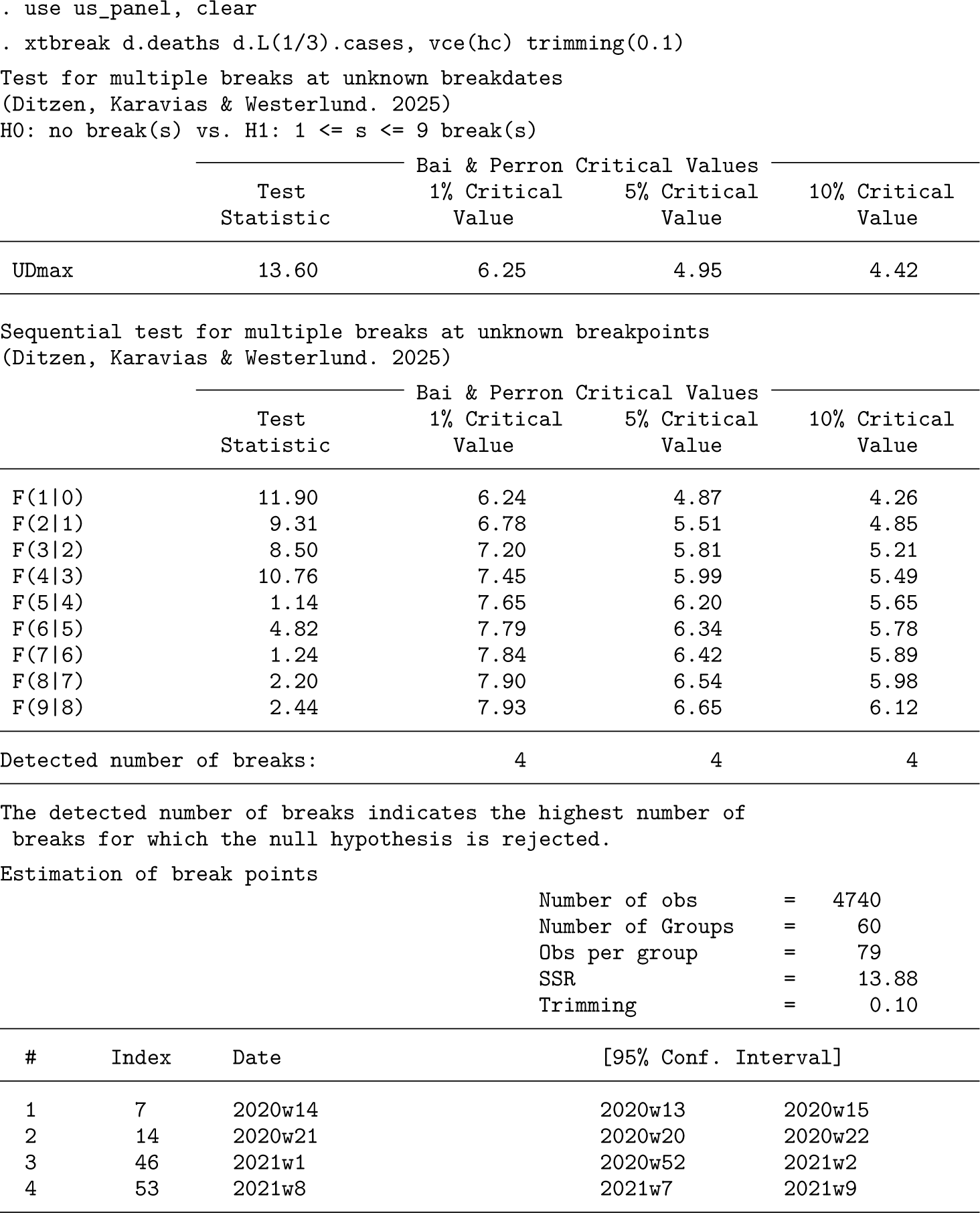
Like before, we report some results based on the sequential test to estimate the number of breaks and the break dates. We begin with the automatic xtbreak command that tests hypothesis 3 sequentially. The default panel-data case assumes no serial correlation or cross-sectional dependence. It has no constant but includes fixed effects. The distributed lag model used here captures serial correlation, so we use only heteroskedasticity-robust standard errors. Additionally, we use a smaller trimming of 10%. ¹⁶ xtbreak automatically detects whether a panel-data model is used, and thus the syntax remains the same. These are the results:

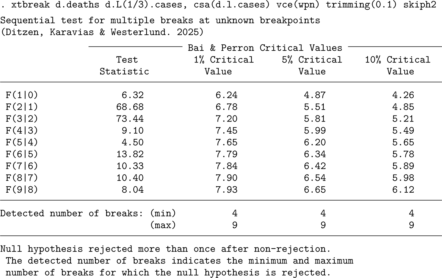
At a 5% significance level, we find four breaks that are estimated in weeks 14 and 21 of 2020 and in weeks 1 and 8 of 2021. The second and third breaks are remarkably close to the two breaks found in the single-time-series analysis above. ¹⁷ We will comment on the break dates below. Given that COVID-19 waves impact multiple states at the same time, there may be dependence across states. We address this issue by augmenting the model with the cross-sectional average of the lagged number of differenced cases. ¹⁸ Additionally, we use the option strict, which uses the sequential test until it does not reject the null at the required significance level. strict provides the consistent number of breaks estimator of theorem 3.2 in Ditzen, Karavias, and Westerlund (2025). We also use the skiph2 option, which skips the test of no breaks against 1 < s < s_max breaks to save space because it strongly rejects. We use the heteroskedasticity- and autocorrelation-robust variance estimator of Westerlund, Petrova, and Norkute (2019) because of its excellent small-sample properties. The results look as follows:

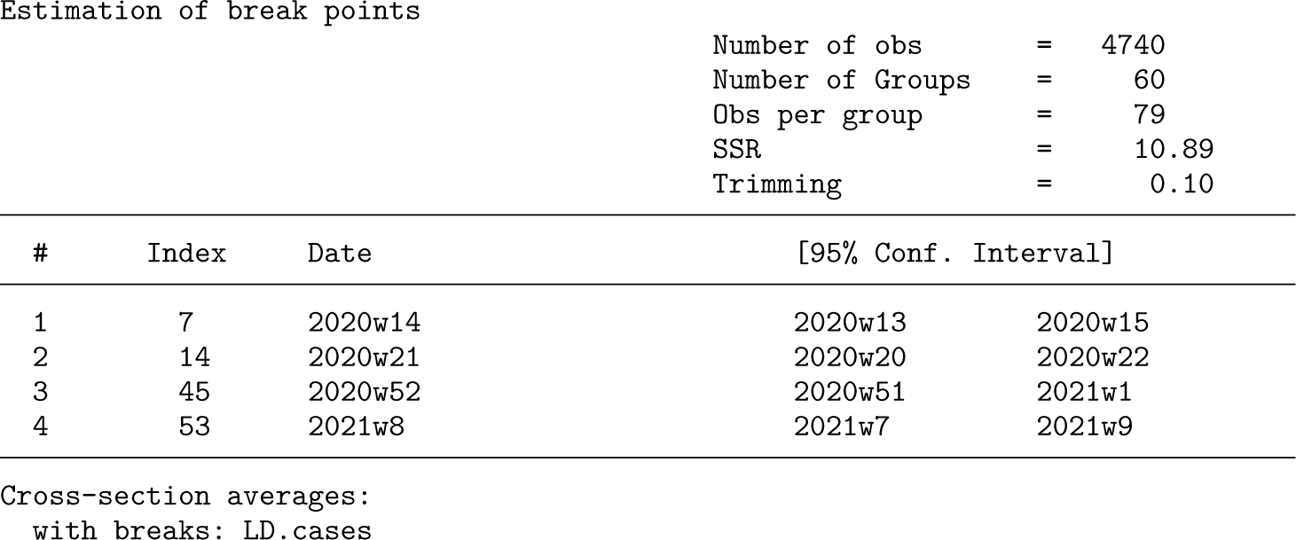
The option strict has a default significance level of 5%. For this significance level, the F(5|4) test does not reject, and the sequential procedure stops yielding an estimate of four breaks. Notably, the breaks are the same as before.

Additional results and discussions

The estimated breaks take place in week 14 of 2020, week 21 of 2020, week 52 of 2020, and week 8 of 2021. The confidence intervals for all four breaks are narrow. When we compare these results with those reported earlier for the time-series dataset for the whole US, we see that the second and third breaks coincide. Hence, for two of the break dates, the panel-data evidence reinforces the time-series evidence reported earlier. However, the panel-data results also suggest that two breaks are not enough and that there is a need to account for an early break in week 14 of 2020 and for a fourth break in week 8 of 2021. The fact that the panel toolbox detects two breaks that are not picked up by the time-series analysis could be due to the gain in accuracy obtained by using the larger panel dataset (see Ditzen, Karavias, and Westerlund [2025]).

The command estat split generates the breaking regressors that will be used as independent variables. The model is fit by CCE using xtdcce2 (Ditzen 2018, 2021) because the CCE estimator allows for interactive effects that capture cross-section dependence. As with the above, we report the long-run multipliers for each regime. The estimated multiplier in the first regime, which corresponds to the period of the first wave, is the highest because there was little medical knowledge about the virus at that time, limited preparedness, and limited capacity in detecting cases. The last can be seen in figure 4. The multipliers drop in the second regime as the first wave dissipates and more testing becomes available. The third regime includes the second and part of the third wave appearing in October 2020. The multiplier further drops here. The fourth regime includes the peak of the third wave. Here cases and deaths are close to each other because of extensive tracing programs used across states and also mass vaccinations. The multiplier remains almost the same in the fifth and final regime. This is an example of a break that is statistically significant but may not be economically significant, so we do not consider more breaks in the analysis. ¹⁹

Figure 4.

Plotting estimated breaks (dashed lines), 95% confidence intervals (dotted lines), deaths, and lagged cases. The arrows on top indicate the regimes.

7 Consumer confidence and leader approval rating

Another relationship that can potentially suffer from structural breaks is that between consumer confidence and the approval rating of a country’s leader. In the US, there is now a large literature analyzing the determinants of presidential ratings (see, for example, Berlemann and Enkelmann [2014] for an extensive review). The determinant of interest here is consumer confidence, a statistical measure of consumer feelings on the state of the economy and their financial situation. Confidence in the economy should translate into high presidential ratings, although the relationship itself may be unstable at times with structural breaks occurring for various reasons, including political instability and other significant events, an example being the inauguration of President Barack Obama (Small and Eisinger 2020). Another dimension of interest when studying such relationships is their cross-country heterogeneity, which is the outcome of unique historical processes shaping institutions and culture. In the words of Nannestad and Paldam (1994), “approval relationships have shown a disappointing lack of stability both over time and across countries.”

The present study is motivated by the above discussion and will attempt to discover breaks in a set of eight countries in which leader approval ratings were observed monthly from January 1990 to December 2021. The data on approval ratings were obtained from the EAP 3.0 database (Carlin et al. 2023), while the data on consumer confidence were taken from the OECD. ²⁰ The two variables are denoted as approval and CCI. Because the time dimension is long, we set the trimming parameter to 5%. Additionally, we control for breaks because of elections, which can be seen as known break dates. Election dates for the years after 2000 come from the International Foundation for Electoral Systems (2023) and are entered manually for the years before 2000. To account for the political environment right before and after an election, the dummy variable ElectionQ equals 1 in the month before an election and for the two months after an election. We analyze first the whole panel and then each country separately.

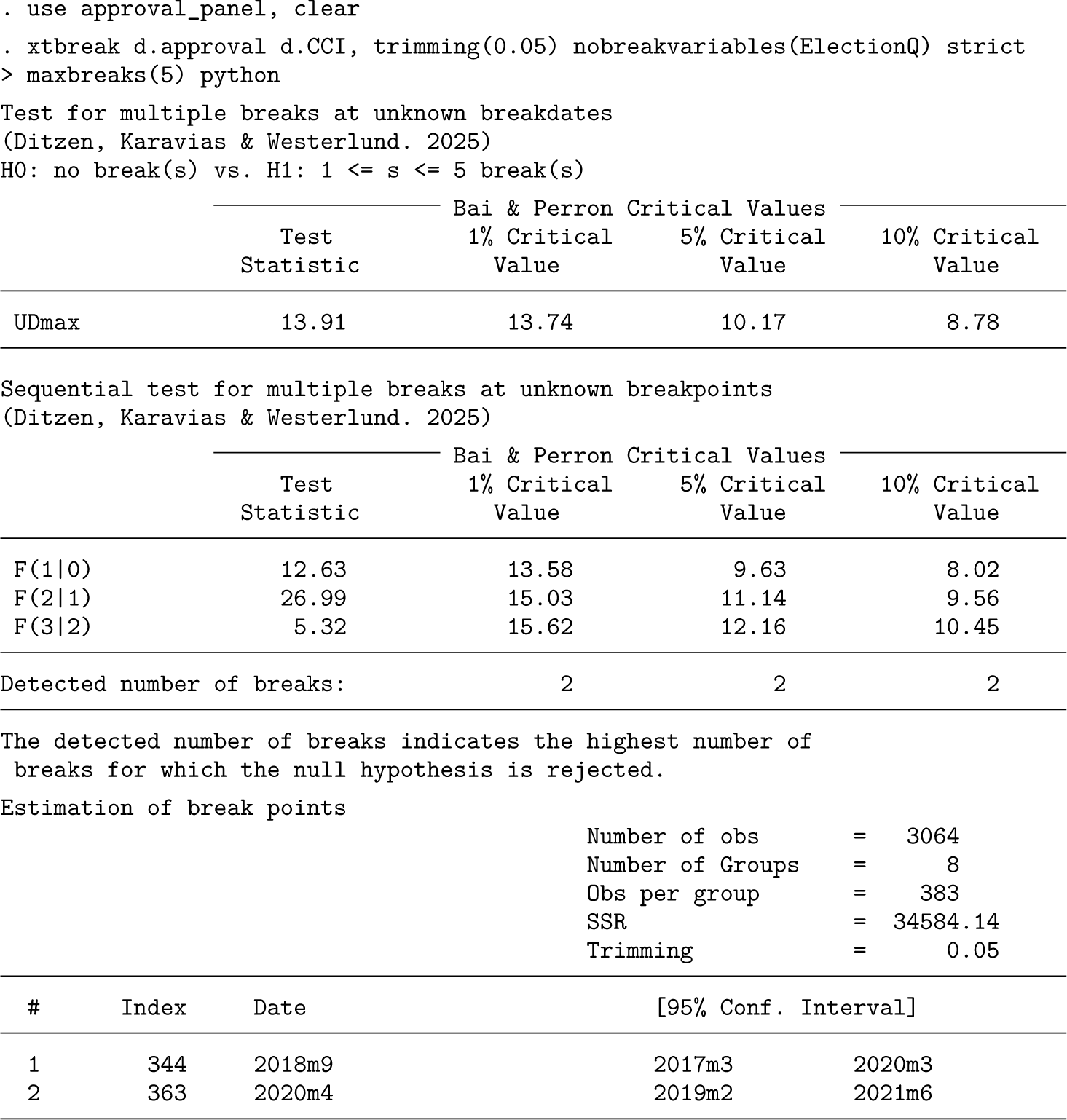
In the estimations below, we allow unobserved heterogeneity to account for country-specific variation and use first differences of the variables to ensure stationarity. Because the time dimension is large, many possible SSRs must be estimated, which takes a considerable amount of time. ²¹ To save time, we restrict the number of breaks under the null hypothesis for hypothesis 2 to s_max = 5 using the options maxbreaks(5) and strict for the sequential test and invoke the option python. ²² With the strict option, the sequential test will stop once the null hypothesis F(s + 1|s) is not rejected given a rejection of F(s|s − 1) at the default 5% significance level.

The UDmax test is rejected at the 10% level, suggesting at least one break in the relationship. Such evidence is rather weak given the size of the sample. However, looking at the sequential statistic results, there is strong evidence in favor of two breaks at all significance levels. The two breaks are found in September 2018 and April 2020. In both cases, the confidence intervals of the breaks span more than one year, having a width of 36 and 28 months, respectively. The first break could be due to Donald Trump’s election in the US; its confidence interval includes almost his entire first presidency. Trump’s election is significant because leaders across the board try to side with or oppose his rhetoric and policies. The second break could be due to the COVID-19 pandemic, which was a difficult and multifaceted problem for leaders and the economy.

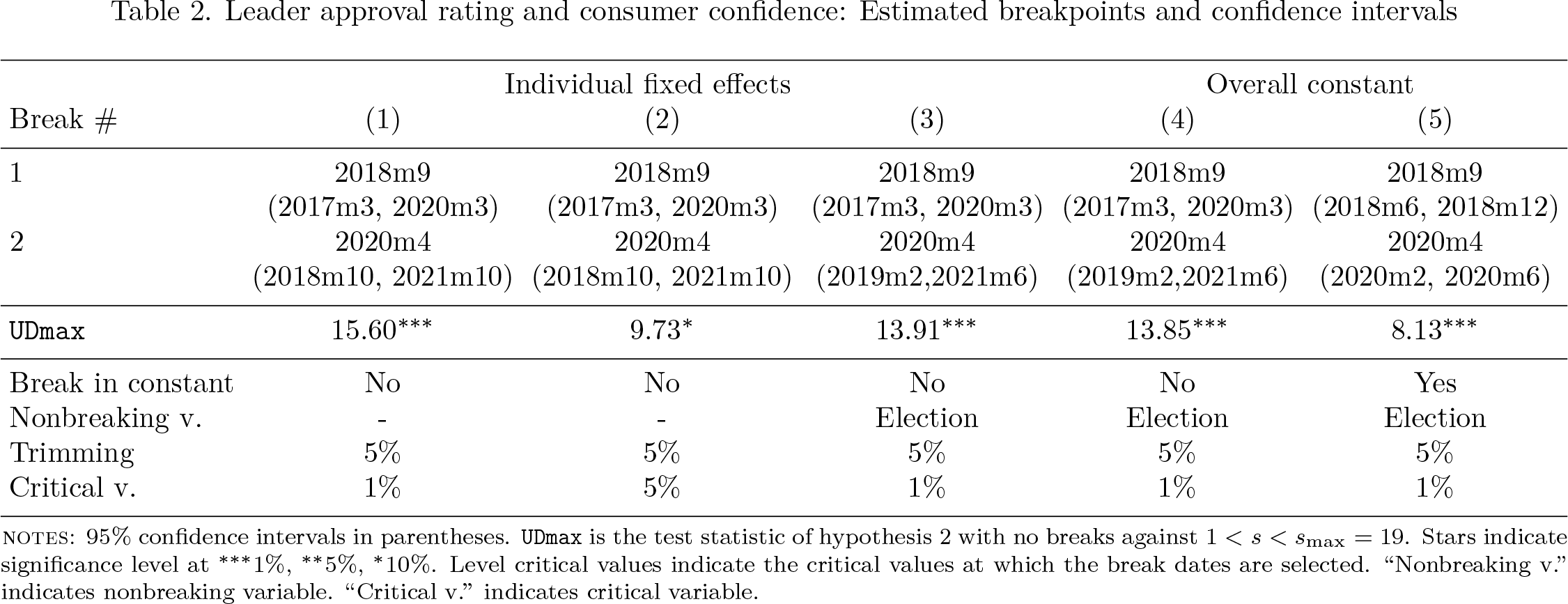
Table 2 presents some further robustness results examining how the number and location of breaks vary across model specifications. The parameters that vary are trimming, the constant or fixed-effects specification, the significance level, and whether “Elections” are included as the nonbreaking regressor. Overall, we observe that the panel results are robust to these choices.

Table 2.

Leader approval rating and consumer confidence: Estimated breakpoints and confidence intervals

	Individual fixed effects			Overall constant
Break #	(1)	(2)	(3)	(4)	(5)
1	2018m9 (2017m3, 2020m3)	2018m9 (2017m3, 2020m3)	2018m9 (2017m3, 2020m3)	2018m9 (2017m3, 2020m3)	2018m9 (2018m6, 2018m12)
2	2020m4 (2018m10, 2021m10)	2020m4 (2018m10, 2021m10)	2020m4 (2019m2,2021m6)	2020m4 (2019m2,2021m6)	2020m4 (2020m2, 2020m6)
UDmax	15.60***	9.73*	13.91***	13.85***	8.13***
Break in constant	No	No	No	No	Yes
Nonbreaking v.	-	-	Election	Election	Election
Trimming	5%	5%	5%	5%	5%
Critical v.	1%	5%	1%	1%	1%

notes: 95% confidence intervals in parentheses. UDmax is the test statistic of hypothesis 2 with no breaks against 1 < s < s_max = 19. Stars indicate significance level at ***1%, **5%, *10%. Level critical values indicate the critical values at which the break dates are selected. “Nonbreaking v.” indicates nonbreaking variable. “Critical v.” indicates critical variable.

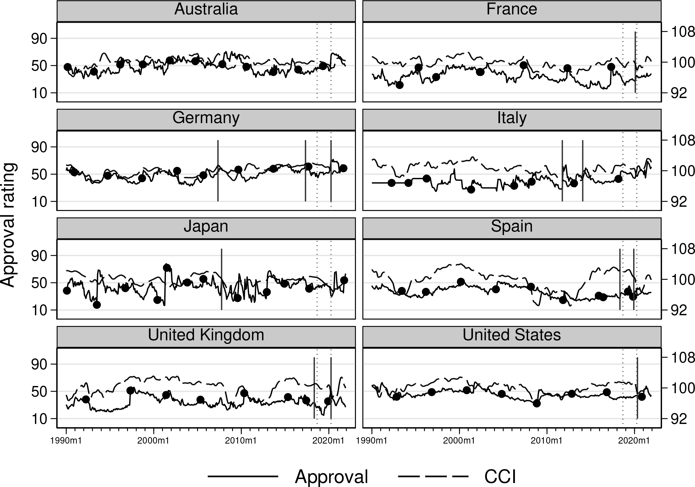
We now explore cross-country heterogeneity by analyzing the disaggregated data for each of the eight countries in the sample. Individual country analysis allows for heterogeneous intercept and slope regression coefficients, although it can be less efficient. The results are depicted in figure 5, which includes the estimated break dates marked by vertical lines because they have been estimated in each time series. For comparison, the estimated breaks of the full panel are indicated by a dotted line. The number of estimated breaks ranges from none (Australia) to three (Germany). The April 2020 break estimated in the panel appears in five of eight countries: France, Germany, Spain, the UK, and the US. The break in 2018 appears only in Spain and the UK. Overall, the figure shows that the heterogeneity across countries is significant.

Figure 5.

Leader confidence. Dashed lines indicate break-point estimates on country level; dotted lines indicate the same on panel level; and dots indicate elections.

Figure 6.

SSRs over time

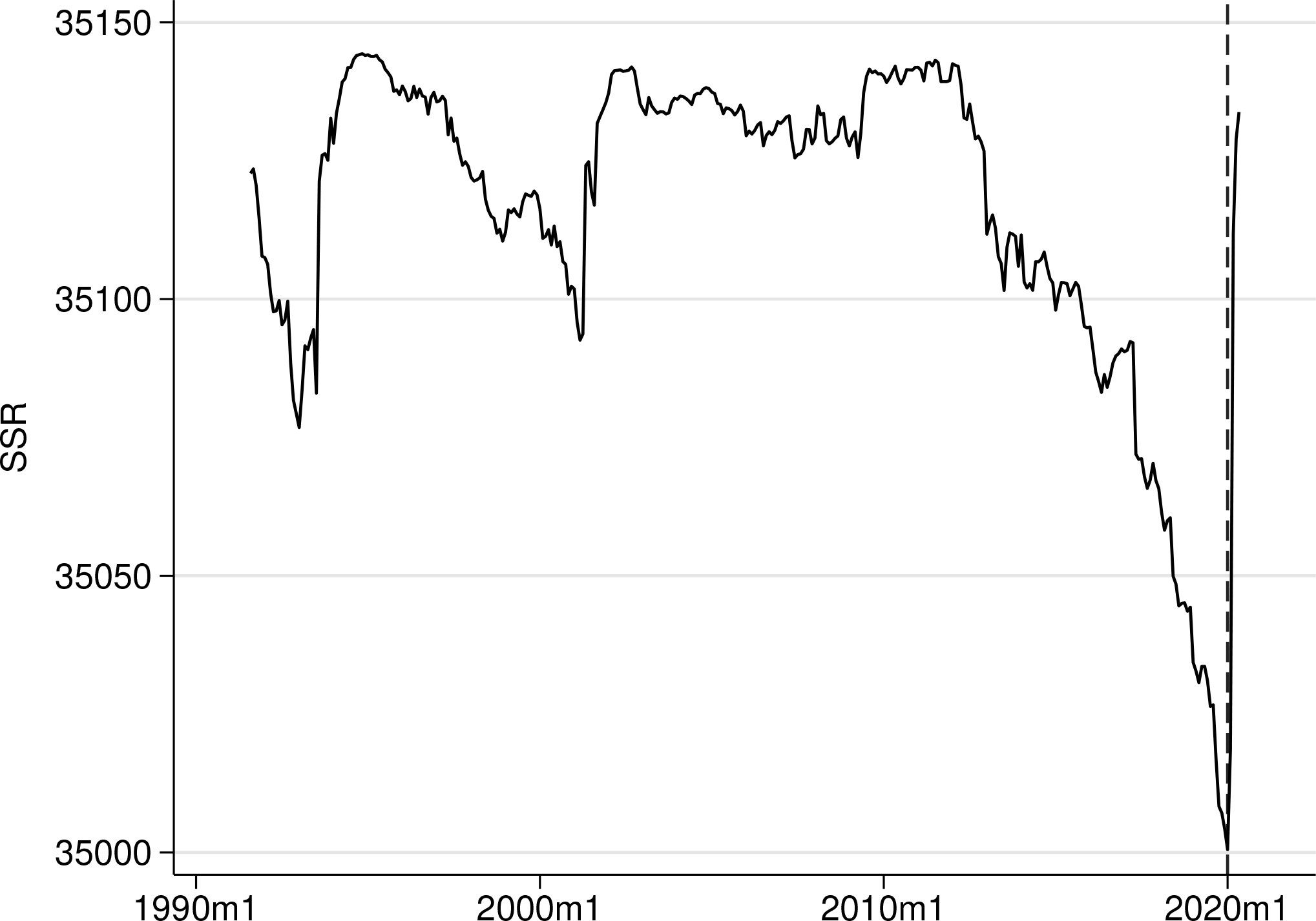
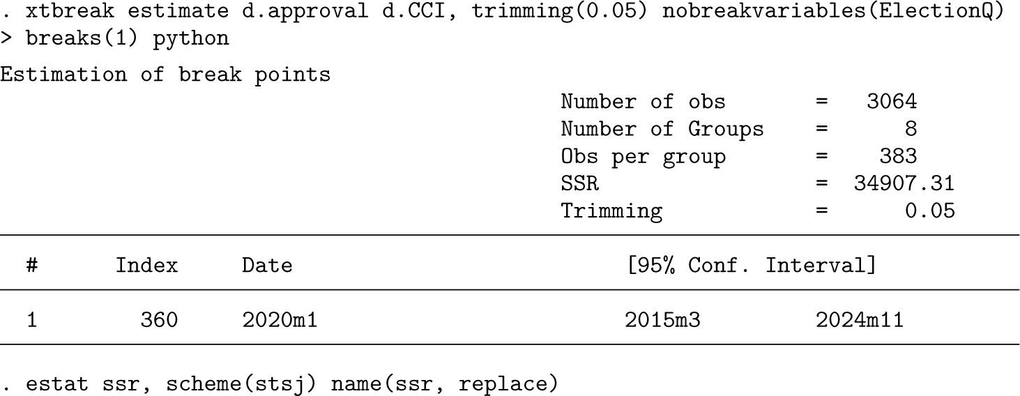
As a final exercise, we return to the panel case and assume that there is a single break. We now plot the SSRs via estat ssr after using xtbreak estimate. The estat ssr command is available only after the estimation of a single break and displays the SSR for each possible break date. ²³

The estimated break point is indicated by a dashed line. The break is estimated to be in January 2020, and the SSR of 34907.31 represents the sum of the SSR of an estimation ranging from January 1990 until January 2020 and the SSR of an estimation from February 2020 to December 2021. This break is almost identical to the second break in the panel-data model above and coincides with the second break appearing in five out of the eight countries of the sample. In an underspecified model in which the assumed number of breaks is less than the true number of breaks, the break-date estimators are still consistent for the true break dates (see Bai and Perron [1998]). Therefore, the estimator of the one break here is meaningful and converges to one of the true break points; which of the true breaks it will converge to depends on the magnitudes of the breaks and the duration of the regimes.

8 Conclusion

This article presents a new community-contributed command called xtbreak, which enables researchers to detect breaks and estimate their number and location. The command can be applied to time series and panel data and can hence be seen as a complete break detection toolbox that is applicable regardless of the structure of the data. The xtbreak command is applied to detect breaks in the relationship between COVID-19 cases and deaths and in the relationship between consumer confidence and the approval ratings of country leaders.

In the following, we discuss challenges, limitations, and further research ideas that are relevant to the current contribution. Computational speed can be a challenge, especially in datasets with many time-series observations. The dynamic programming algorithm embedded in xtbreak goes far in addressing this issue because it ensures that at most O(T²) calculations are made when the number of breaks is more than two; however, this number can still be large. xtbreak includes several options that can further improve computational speed, such as the use of Python or the use of faster but less precise matrix inversion methods. Speed gains can also be achieved through modeling choices: the pure structural-break model computes significantly faster than the partial break model. Consequently, it may be advantageous to assume that breaks affect all coefficients rather than just a subset. While assuming a coefficient break when none exists does not lead to inconsistent estimation, it does result in inefficiency; therefore, this option should be exercised with caution. Future research could explore additional speed improvements through multiprocess parallelization, which is something not explored thus far.

The panel-data methodology used in this article assumes common coefficients and common breaks across units. This is the prevalent setting in the applied literature; however, there are situations where heterogeneity is a significant feature of the data. Recently, steps have been taken to relax these assumptions; see, for example, Okui and Wang (2021), who propose a model in which different groups of units suffer a different number of breaks at different times. This method has not been coded in Stata so far, and it would be an important complement to the methodology in this article.

Supplemental Material

sj-dta-1-stj-10.1177_1536867X251365449 - Supplemental material for Testing and estimating structural breaks in time series and panel data in Stata

Supplemental material, sj-dta-1-stj-10.1177_1536867X251365449 for Testing and estimating structural breaks in time series and panel data in Stata by Jan Ditzen, Yiannis Karavias and Joakim Westerlund in The Stata Journal

Supplemental Material

sj-dta-2-stj-10.1177_1536867X251365449 - Supplemental material for Testing and estimating structural breaks in time series and panel data in Stata

Supplemental material, sj-dta-2-stj-10.1177_1536867X251365449 for Testing and estimating structural breaks in time series and panel data in Stata by Jan Ditzen, Yiannis Karavias and Joakim Westerlund in The Stata Journal

Supplemental Material

sj-dta-3-stj-10.1177_1536867X251365449 - Supplemental material for Testing and estimating structural breaks in time series and panel data in Stata

Supplemental material, sj-dta-3-stj-10.1177_1536867X251365449 for Testing and estimating structural breaks in time series and panel data in Stata by Jan Ditzen, Yiannis Karavias and Joakim Westerlund in The Stata Journal

Supplemental Material

sj-txt-1-stj-10.1177_1536867X251365449 - Supplemental material for Testing and estimating structural breaks in time series and panel data in Stata

Supplemental material, sj-txt-1-stj-10.1177_1536867X251365449 for Testing and estimating structural breaks in time series and panel data in Stata by Jan Ditzen, Yiannis Karavias and Joakim Westerlund in The Stata Journal

References

1.
BaiJ. 2009. Panel data models with interactive fixed effects. Econometrica77: 1229–1279. 10.3982/ECTA6135.
2.
BaiJ.PerronP.. 1998. Estimating and testing linear models with multiple structural changes. Econometrica66: 47–78. 10.2307/2998540.
3.
——. 2003. Computation and analysis of multiple structural change models. Journal of Applied Econometrics18: 1–22. 10.1002/jae.659.
4.
BerlemannM.EnkelmannS.. 2014. The economic determinants of U.S. presidential approval: A survey. European Journal of Political Economy36: 41–54. 10.1016/j.ejpoleco.2014.06.005.
DitzenJ. 2018. Estimating dynamic common-correlated effects in Stata. Stata Journal18: 585–617. 10.1177/1536867X1801800306.
7.
——. 2021. Estimating long-run effects and the exponent of cross-sectional dependence: An update to xtdcce2. Stata Journal21: 687–707. 10.1177/1536867X211045560.
8.
DitzenJ.KaraviasY.WesterlundJ.. 2025. Multiple structural breaks in interactive effects panel data models. Journal of Applied Econometrics40: 74–88. 10.1002/jae.3097.
9.
FritzM. 2022. Wave after wave: Determining the temporal lag in Covid-19 infections and deaths using spatial panel data from Germany. Journal of Spatial Econometrics3: art. 9.10.1007/s43071-022-00027-6.
JannB.2005. moremata: Stata module (Mata) to provide various functions. Statistical Software Components S455001, Department of Economics, Boston College. https://ideas.repec.org/c/boc/bocode/s455001.html.
12.
KaraviasY.NarayanP. K.WesterlundJ.. 2023. Structural breaks in interactive effects panels and the stock market reaction to COVID-19. Journal of Business and Economic Statistics41: 653–666. 10.1080/07350015.2022.2053690.
13.
MathieuE.RitchieH.Rodés-GuiraoL.AppelC.GiattinoC.HasellJ.MacdonaldB.DattaniS.BeltekianD.Ortiz-OspinaE.RoserM.. 2020. COVID-19 Pandemic. Our World in Data. https://ourworldindata.org/coronavirus.
14.
NannestadP.PaldamM.. 1994. The VP-function: A survey of the literature on vote and popularity functions after 25 years. Public Choice79: 213–245. 10.1007/BF01047771.
15.
OkuiR.WangW.. 2021. Heterogeneous structural breaks in panel data models. Journal of Econometrics220: 447–473. 10.1016/j.jeconom.2020.04.009.
16.
PesaranM. H. 2006. Estimation and inference in large heterogeneous panels with a multifactor error structure. Econometrica74: 967–1012. 10.1111/j.1468-0262.2006.00692.x.
17.
SilverioA.Di MaioM.CiccarelliM.CarrizzoA.VecchioneC.GalassoG.. 2020. Timing of national lockdown and mortality in COVID-19: The Italian experience. International Journal of Infectious Diseases100: 193–195. 10.1016/j.ijid.2020.09.006.
18.
SmallR.EisingerR. M.. 2020. Whither presidential approval?Presidential Studies Quarterly50: 845–863. 10.1111/psq.12680.
19.
WesterlundJ.PetrovaY.NorkuteM.. 2019. CCE in fixed-T panels. Journal of Applied Econometrics34: 746–761. 10.1002/jae.2707.
Supplementary Material
Please find the following supplemental material available below.
For Open Access articles published under a Creative Commons License, all supplemental material carries the same license as the article it is associated with.
For non-Open Access articles published, all supplemental material carries a non-exclusive license, and permission requests for re-use of supplemental material or any part of supplemental material shall be sent directly to the copyright owner as specified in the copyright notice associated with the article.