Sage Journals: Discover world-class research

Abstract

We introduce HistoNet, a deep neural network trained on normal tissue. On 1690 slides with rat tissue samples from 6 preclinical toxicology studies, tissue regions were outlined and annotated by pathologists into 46 different tissue classes. From these annotated regions, we sampled small 224 × 224 pixels images (patches) at 6 different levels of magnification. Using 4 studies as training set and 2 studies as test set, we trained VGG-16, ResNet-50, and Inception-v3 networks separately at each magnification level. Among these model architectures, Inception-v3 and ResNet-50 outperformed VGG-16. Inception-v3 identified the tissue from query images, with an accuracy up to 83.4%. Most misclassifications occurred between histologically similar tissues. Investigation of the features learned by the model (embedding layer) using Uniform Manifold Approximation and Projection revealed not only coherent clusters associated with the individual tissues but also subclusters corresponding to histologically meaningful structures that had not been annotated or trained for. This suggests that the histological representation learned by HistoNet could be useful as the basis of other machine learning algorithms and data mining. Finally, we found that models trained on rat tissues can be used on non-human primate and minipig tissues with minimal retraining.

Keywords

histopathology histology computational pathology machine learning deep learning

Introduction

After breakthrough results in the ImageNet challenge 2012¹ and subsequent challenges, deep neural networks have led to a radical transformation of many scientific disciplines, including medicine. In particular, deep learning-based diagnostics have achieved physician-level accuracy across a wide range of diagnostic tasks,^2,3 and the potential of deep learning to transform health care has been broadly recognized by regulatory agencies as well as in the literature.^4,5

Computational pathology is defined as an approach to diagnosis that incorporates multiple sources of raw data.⁶ A key element of the approach is the ability to derive data from histopathology images. Deep learning is potentially an accelerator of the development of computational pathology⁷ but faces specific challenges posed by whole-slide imaging (WSI) of tissue sections stained with hematoxylin and eosin (H&E) including large image sizes, color variation and other artifacts, and, more importantly, the multiscale nature of the data—with various emergent structures from the nuclei to the organ level.⁸ Moreover, obtaining annotations is more challenging for histopathology than in other disciplines: It is highly time-consuming and requires input from trained pathologists.

To date, the bulk of machine learning approaches to digital pathology has focused on detection and segmentation of histologic elementary components such as nuclear size and shape, grading of lesions,⁹ prediction of clinical outcomes, and linking histopathology with other data types.^8,10 Recent community challenges aimed at detecting lymph node metastases,^11,12 assessing tumor proliferation in breast cancer,¹³ or detecting and classifying lung cancer.¹⁴ Other recent work has explored the prediction of genetic alterations from H&E-stained slides.^15,16

All of these applications operate in a disease-specific context, which presupposes a histopathological diagnosis to be established prior to submitting slides to the application. That is, the morphological features learned by such models are optimized for the differentiation of specific outcomes given the initial diagnosis. Therefore, it is difficult to imagine how such models could contribute to applications aiming at assisting the diagnosis, that is, identify key diagnostic features from a nonpredetermined histopathological slide. In contrast, a model based on features that differentiate all possible tissue characteristics pertaining to identifying any type of tissue or histological lesion would provide invaluable support for the development of applications to assist in pathological diagnosis. The mere automated identification of samples devoid of lesion could tremendously improve the efficiency and quality of pathology evaluation in areas of clinical practice providing screening for lesions but also in preclinical development of medicines, where pathology is pivotal for the assessment of drug safety.

Our work focused on the development of a holistic model of histology—HistoNet—which, from our perspective, will lay the foundation of more complex models suitable for assistance to diagnosis in both toxicologic pathology and clinical medicine. Working from preclinical toxicology studies offered a unique opportunity to obtain a systematic collection of all normal tissues at high quality and from multiple species. These data sets allowed us to develop holistic tissue models and explore the morphological differences between species. This was particularly useful since obtaining a complete and homogeneous set of normal human tissues through autopsies is hindered by several factors, including the necessary consents, the age of the patients, or the delays between death and collection.

The 3 key contributions of this article are the following:

Tissue Recognition

First, we show that a comprehensive set of tissues can be recognized by standard convolutional neural networks (CNNs) trained on small images (patches) extracted, at various magnifications from H&E-stained WSI of a diversity of rat tissues. We use the term HistoNet(s) for these deep learning-based models of histology. The Inception-v3 and ResNet-50 CNN architectures outperformed VGG-16. The Inception-v3 network showed a patch-level test set accuracy of up to 83.4% (top-3 accuracy: 96.3%) on an independent test set and was used for the subsequent analyses.

Analysis of Neural Network Embeddings

In a CNN, the input image is transformed through several stages into a high-dimensional vector of image features learned during training and stored in the penultimate layer. This vector is typically referred to as the “embedding.” We collected these embedding vectors for all patches from the rat test set and visualized them. As a high-dimensional vector cannot be plotted directly, we used nonlinear dimensionality reduction techniques to generate 2-dimensional interactive plots that pathologists used to validate the models and explore relationships in the data. Patches from the same tissue formed 1 or more groups, often distinct from other tissues. Overlaps between groups often corresponded to similar histological structures present in more than 1 tissue. More in-depth exploration of the embeddings revealed that HistoNet had learned a representation for histologically relevant substructures that had neither been annotated nor trained for.

Cross-Species Predictions and Transfer Learning

Using control animals from studies in minipig and non-human primates (NHP), we first show that the rat version of HistoNet is able to recognize some tissues in other species without any species-specific fine-tuning, but that overall tissue recognition does not generalize well across species. We then investigate species-specific fine-tuning and demonstrate that the rat HistoNet model leads to improved accuracy with reduced amounts of required training data, as compared to a generic ImageNet model. We suggest that similar observations will hold true for other machine learning tasks in a histopathological context, for which a HistoNet might thus provide a more suitable starting point than an ImageNet model.

Materials and Methods

Data Set

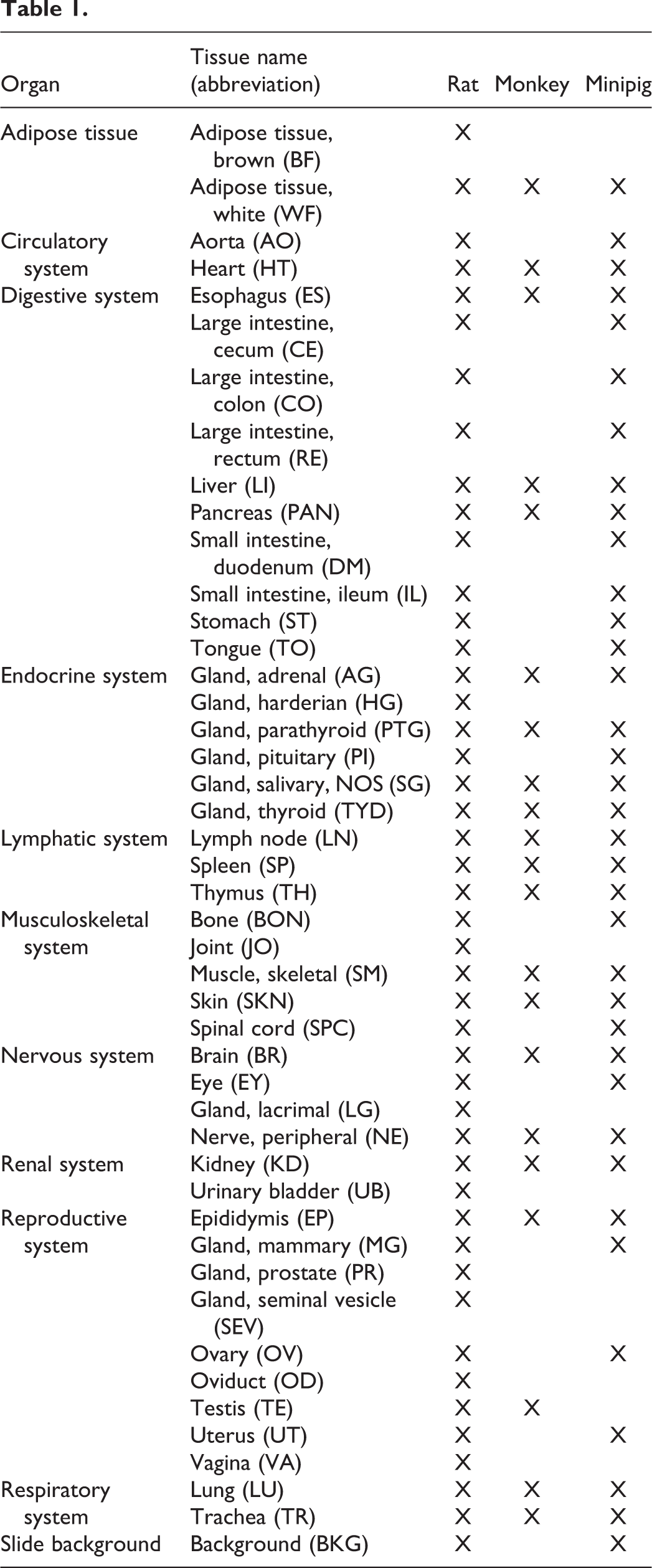
Hematoxylin and eosin–stained slides from independently processed preclinical toxicology studies were retrieved from archives. All individual studies had been previously approved by an ethics review board as required. To establish the rat models, 6 studies performed in Han-Wistar rats (Rattus norvegicus) provided 1690 WSIs of 46 different tissues with at least 20 slides per tissue, covering 9 organ systems (Table 1; for simplicity, the slide background was included as a tissue class). Organs representing subtle variation of tissue structure (such as different segments of the intestine) or complex arrangements of tissues (eye, joint [JO]) were intentionally included as extreme cases.

Table 1.

Organ	Tissue name (abbreviation)	Rat	Monkey	Minipig
Adipose tissue	Adipose tissue, brown (BF)	X
Adipose tissue	Adipose tissue, white (WF)	X	X	X
Circulatory system	Aorta (AO)	X		X
Circulatory system	Heart (HT)	X	X	X
Digestive system	Esophagus (ES)	X	X	X
	Large intestine, cecum (CE)	X		X
	Large intestine, colon (CO)	X		X
	Large intestine, rectum (RE)	X		X
	Liver (LI)	X	X	X
	Pancreas (PAN)	X	X	X
	Small intestine, duodenum (DM)	X		X
	Small intestine, ileum (IL)	X		X
	Stomach (ST)	X		X
	Tongue (TO)	X		X
Endocrine system	Gland, adrenal (AG)	X	X	X
	Gland, harderian (HG)	X
	Gland, parathyroid (PTG)	X	X	X
	Gland, pituitary (PI)	X		X
	Gland, salivary, NOS (SG)	X	X	X
	Gland, thyroid (TYD)	X	X	X
Lymphatic system	Lymph node (LN)	X	X	X
	Spleen (SP)	X	X	X
	Thymus (TH)	X	X	X
Musculoskeletal system	Bone (BON)	X		X
	Joint (JO)	X
	Muscle, skeletal (SM)	X	X	X
	Skin (SKN)	X	X	X
	Spinal cord (SPC)	X		X
Nervous system	Brain (BR)	X	X	X
	Eye (EY)	X		X
	Gland, lacrimal (LG)	X
	Nerve, peripheral (NE)	X	X	X
Renal system	Kidney (KD)	X	X	X
Renal system	Urinary bladder (UB)	X
Reproductive system	Epididymis (EP)	X	X	X
	Gland, mammary (MG)	X		X
	Gland, prostate (PR)	X
	Gland, seminal vesicle (SEV)	X
	Ovary (OV)	X		X
	Oviduct (OD)	X
	Testis (TE)	X	X
	Uterus (UT)	X		X
	Vagina (VA)	X
Respiratory system	Lung (LU)	X	X	X
Respiratory system	Trachea (TR)	X	X	X
Slide background	Background (BKG)	X		X

Four studies were selected for the training data set (1183 slides) and 2 for the test data set (507 slides). To evaluate the cross-species translatability and species-specific models, WSIs from minipig (Sus scrofa domesticus) and cynomolgus NHP (Macaca fascicularis) were generated from the control arm of 1 (minipig) and 2 (NHP) studies, covering subsets of 36 and 21 tissues, respectively. As the sizes of the studies are very different as well as not all tissues being available in each study, the studies were selected in order to guarantee similar numbers of slides for each tissue in training as well as test set.

Whole-slide images were generated at ×40 magnification (0.252 microns per pixel [mpp]) using either Aperio or Hamamatsu scanners. All WSIs were reviewed by pathologists to ensure the absence of lesions. Then, tissues were outlined manually (using Indica Labs Halo or Aperio Imagescope) and labeled according to a catalog of tissue types (see Table 1) by several pathologists. These manual outlines defined regions corresponding to individual tissues on the WSIs from which patches of size 224 × 224 pixels were extracted at the various magnification levels corresponding to 0.252, 0.504, 1.008, 2.016, 4.032, and 8.064 mpp (×40 down to ×1.25; Figure 1A). As the pixel size of patches is constant across all magnifications, low-magnification (high mpp) patches cover a larger area of the underlying slide as compared to high-magnification patches. For example, a patch at 0.252 mpp covers an area of 56.4 × 56.4 µm on the slide, while a patch created at 8.064 mpp covers an area of 1.8 mm × 1.8 mm (7168 × 7168 pixels at the original scanning magnification).

Figure 1.

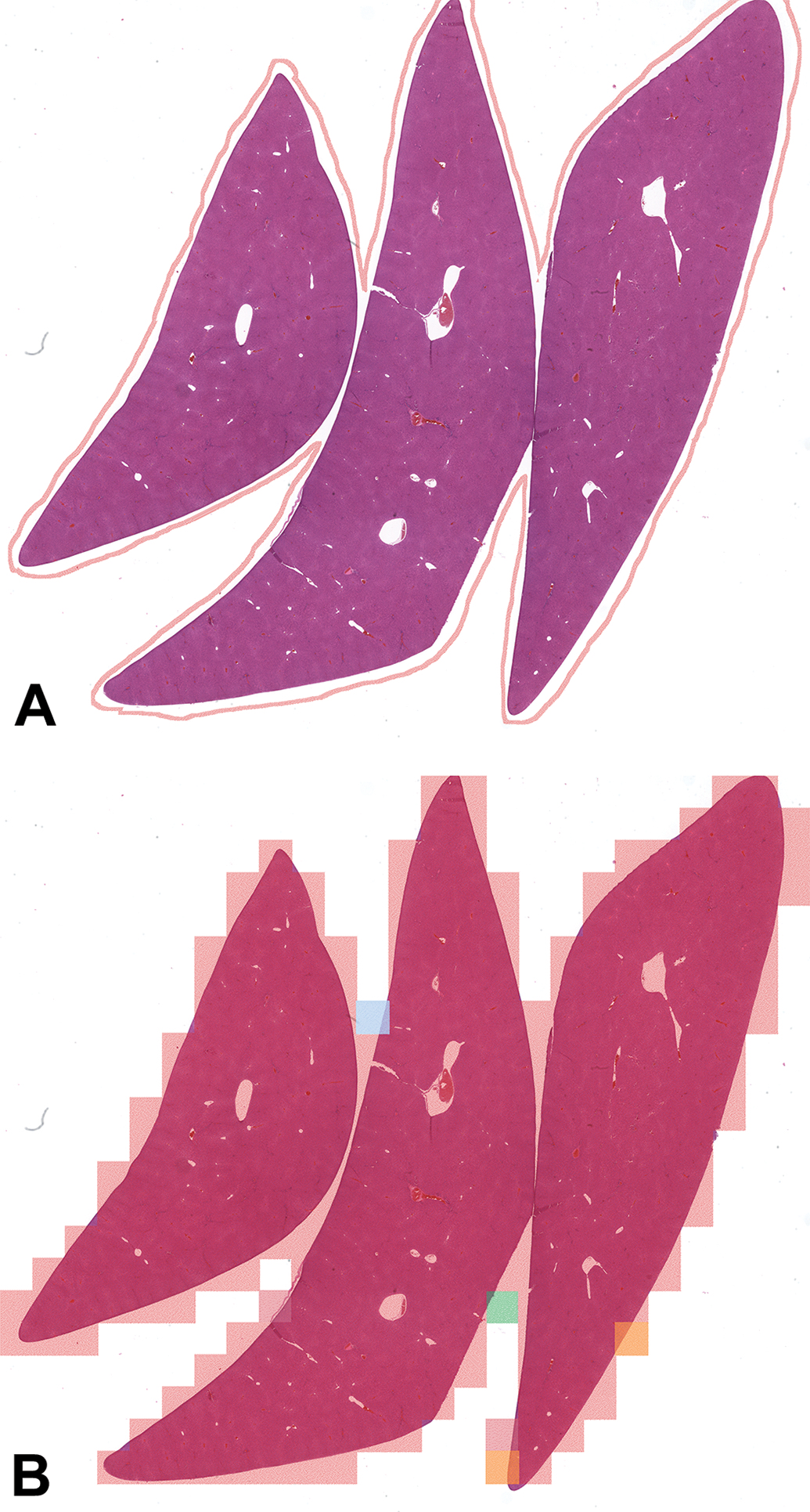
Image of liver tissue with the outline created by pathologists (A). Image of the same tissue with results of the trained Inception-v3 model at 4.032 mpp overlayed. The large majority of patches are predicted correctly (red rectangles) with some incorrect predictions (orange, green, and blue) mostly occurring at the boundary of the tissue (B).

To support the learning of tissue boundaries, patches were allowed to overlap with the boundary of a tissue: A patch is valid for a region if its center is contained within the region. This approach is suggested by empirical findings of improved predictive performance when incorporating challenging boundary patches into the training set.¹⁷

To ensure that the training and test sets are well balanced, we aimed at having equal numbers of patches for each tissue in each data set (∼30,000 and 2000 patches per tissue in the training and test set, respectively). However, the vastly different macroscopic size of some of these tissues made it problematic to sample the same number of patches for each tissue due to oversampling concerns. For example, in the training set, 32,600 mm² of brain (BR) tissue and 27,200 mm² of lung (LU) tissue were available, in contrast to only 25 mm² of parathyroid gland (PTG) tissue (Supplementary Table 1). In order to address this issue, the following scheme was implemented:

The midpoints of the patches were picked at random from the tissue area. The patches were then generated at all mpp levels for the same patch midpoint and the same random rotation. In order to avoid oversampling for tissues with low areas, the number of patches was decreased so that the average patch density at the mpp level of 0.504 was at most 1. For the training set, 34 of 46 tissues had the full 30,000 patches, another 11 tissues between 10,000 and 30,000 patches, and PTG with about 2000 training patches. For the test set, 2000 patches were sampled, which was low enough to create the full set of patches for each tissue. For a complete list of tissue areas as well as the number of sampled patches for the training and test sets, see Supplementary Table 1.

Machine Learning Approach

For the 3 network architectures adopted in this study, VGG-16, Inception-v3, and ResNet-50, we used their implementations available in keras (with tensorflow backend). The weights trained on the ImageNet data set were used for initialization of the convolutional layers. For all fully connected layers, we used random initialization of the weights. Starting from this initialization, all weights were set as trainable. The total number of weights in the 3 architectures are 134,449,006 (VGG-16), 21,897,038 (Inception-v3), and 23,681,966 (ResNet-50). The final layer has 1 unit for each tissue class (and 1 unit for the additional “slide background” class) and is set to have a softmax activation function with a probability vector as output.

During training, each patch was subjected to a random rotation and a random staining modulation according to the method described by Tellez et al.¹⁸ This is referred to as sample augmentation and aims at rendering the classifiers robust to changes in orientation and variations in staining as well as to make the most efficient use of the available data. The RGB channels of the image patches are scaled to the interval [0,1]. The training and test set patches were created and saved not during but before the learning process and subjected to a random rotation. This was done beforehand in order to avoid having to store additional slide context, which would be necessary for obtaining a novel rotated rectangular patch “on the fly.” This means that in our approach, each patch is used with the same rotation during each training-validation cycle. On the other hand, the stain modulation is performed during the training process (and thus differently also for the same patch across different training-validation cycles) according to the method described by Tellez et al.¹⁸ Briefly, this method is based on first transforming from RGB color space to a color space consisting of 1 channel each for eosin and hematoxylin and a third channel for the remaining color variation. These channels are then modified individually by a random linear transformation with parameters sampled from uniform distributions. Finally, the modified patch is back-transformed into RGB color space. We experimented with different widths for the uniform distributions and found that a parameter choice that doubles the variation reported by Tellez et al.¹⁸ as “typical” resulted in the best generalization ability, while leading to pronounced changes in the visual appearance of the patches. Note that even patches from a single slide will be oriented and stained independently from each other during the training process. Patches from the test set are not subjected to any staining modulations.

For training, we used the Adam optimizer with a learning rate reduction once learning stagnates. We started out with an initial learning rate of 10⁻⁶ and a reduction of the learning rate by a factor 5 after 5 training-validation cycles of no improvement. We applied early stopping after 10 training-validation cycles of no improvement. During training, we updated all weights, not just the fully connected layer weights, thereby tuning the feature extraction stack of the architectures that had been pretrained on ImageNet to be better adapted to histopathology images. The same approach was also employed for the cross-species transfer learning in which we adapted the rat model to NHP. For our training-validation cycle, we chose to use about 120,000 patches in each, which is roughly 10% of the generated training data. The reason is that the common notion of an “epoch” as one run through all data does not quite apply in this setting, since we can create an arbitrary number of random patches from our slides. We, therefore, chose this number in order to have regular and well-spaced validation runs. For the evaluation of our models, we use a single model training run instead of several independent runs from which performances are averaged. This potentially adds some additional variability to the reported performance estimates.

The performance metrics used in this work are accuracy (the fraction of samples for which the predicted class equals the true class), error rate (1 − accuracy), sensitivity for class t (the fraction of samples from class t that are correctly recognized), and positive predictive value (PPV) for class t (the fraction of samples predicted as t that truly belong to class t).

Uniform Manifold Approximation and Projection (UMAP) of the embeddings was based on the software library provided by the UMAP authors (github.com/lmcinnes/umap). For the validation of the models and review of the UMAP, a jupyter dashboard was created that allowed the pathologists to view 2-dimensional projections of the embeddings and visualize the corresponding patches. This allowed them to intuitively navigate this complex space, look into the morphology of the patches, and store their observations for later use.

Results

Tissue Recognition

Our primary objective was to assess the predictive performance of 3 standard neural network architectures, VGG-16,¹⁹ Inception-v3,²⁰ and ResNet-50,²¹ at recognizing a comprehensive catalogue of 46 tissues at different magnifications. In addition, in order to assess how the models perform in complex histology, we have included the brain (BR), eye (EY), and gastrointestinal tract in the training set.

The accuracy of tissue recognition was assessed using manually curated and annotated WSIs from 46 normal rat tissues (Table 1) collected in 6 independent preclinical toxicology studies and split into training (4 studies; 1183 slides) and test (2 studies; 507 slides) sets. Separate models were trained from patches extracted from the outlined tissues at different magnifications ranging from the scanned resolution (0.252 mpp, typically corresponding to ×40 on some scanners) to a 32-fold downsampling (8.064 mpp). As the pixel size of the patches was kept constant (224 × 224 pixels) across magnifications, the actual area sampled from the slide varied from 0.003 to 3.26 mm² and hence also the amount of contextual information available on a patch. For each magnification, VGG-16, Inception-v3, and ResNet-50 networks—initialized on ImageNet—were trained on patches generated at the given magnification.

By visual inspection, model performance was good for many tissue types (Figure 1B). Accuracy of patch classification ranged from 55.1% to 83.4%, depending on magnification and architecture (Figure 2A). It was higher at low magnification, likely due to the higher amount of context available (larger field of view). At all magnification levels, HistoNets based on Inception-v3 and ResNet-50 architectures outperformed those based on VGG-16, with 81.4% and 83.4% accuracy for the classification of individual patches at 8.064 mpp for ResNet-50 and Inception-v3, respectively, as compared to 74.9% for VGG-16. The performance difference between Inception-v3 and Resnet-50 does not give a strong reason to choose one architecture over the other. Therefore, the Inception-v3–based HistoNet models were used as the basis for subsequent analyses, whereas the ResNet-50 variants of HistoNet were applied to specific tasks described elsewhere.²²

Figure 2.

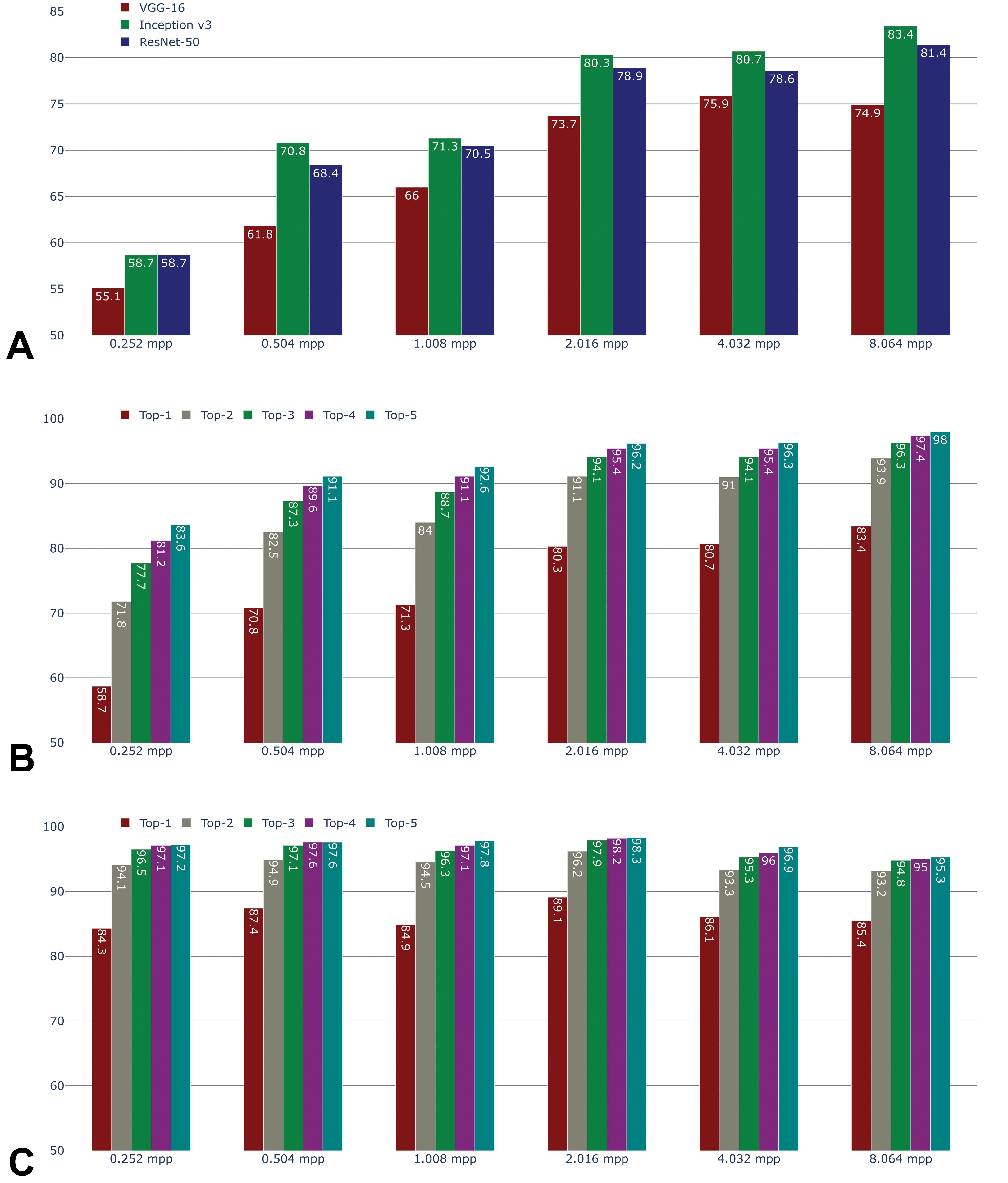
Accuracy of prediction by convolutional neural network architecture and magnification level (A). Accuracy of the top-5 predictions at the patch level by magnification, using the Inception-v3 network (B). Accuracy of the top-5 predictions at the region level by magnification, using the Inception-v3 network (C).

Given that the models were intentionally trained to differentiate morphologically similar tissues such as the different segments of the intestine, the absolute accuracy of tissue prediction may not fully reflect the learning of histologically relevant high-level features. To explore this concept, the top-N accuracy was computed for models based on the Inception-v3 architecture. This standard metric considers a tissue prediction as accurate if the correct class is among the top-N predictions (ranked by the probability assigned to the tissue classes by the network). Informally, the intention is to provide an opportunity for models that are incorrect on their first guess to provide a correct classification with a subsequent guess. In this way, models can be distinguished that are correct on the second or third guess from those that are not. At 8.064 mpp, these accuracies are 83.4% for top-1 (as reported above), 93.9% for top-2, and 96.3% for top-3 (Figure 2B). The performance gap between top-1 and top-2 was particularly large (10.5 percentage points) but subsided between top-2 and top-3 (2.4 percentage points) and even lower for higher N.

Beyond patch classification, we also investigated the predictive performance in the test set at the region level by combining the predictions for all patches extracted from any given tissue outline using a majority vote (Figure 2C). This region-level test set accuracy was much higher than patch-level accuracy for 0.252 and 0.504 mpp, and it generally appeared almost constant across magnifications. Only at 8.064 mpp was the region-level accuracy exceeded by patch-level accuracy. At high resolution, individual patches offer very little field of view, which makes the identification of the tissue more challenging. However, while this means that mistakes are easily made on an individual patch, such errors average out over a large region of the same tissue. Therefore, in this case, region-level accuracy is plausibly higher than patch-level accuracy.

Patch-level sensitivity and PPV for individual tissues showed striking differences varying with magnification (Figure 3). The prediction of morphologically similar regions of the large intestine such as cecum (CE), colon (CO), and rectum (RE) showed low PPV and sensitivity, irrespective of the magnification. This is expected as these labels correspond to the same organ sampled in different locations. The predictions for the femorotibial (JO) and bone (BON) had low PPV and sensitivity at 0.504 and 2.016 mpp, but not at 8.064, probably as patches at this magnification provide a larger field of view that helps identify the arrangement of the various tissue components. Interestingly, the predictions for the parathyroid (PTG) had high PPV and sensitivity at high magnification (0.504 mpp), but while PPV remained high, the sensitivity dropped at 2.016 and further at 8.064 mpp.

Figure 3.

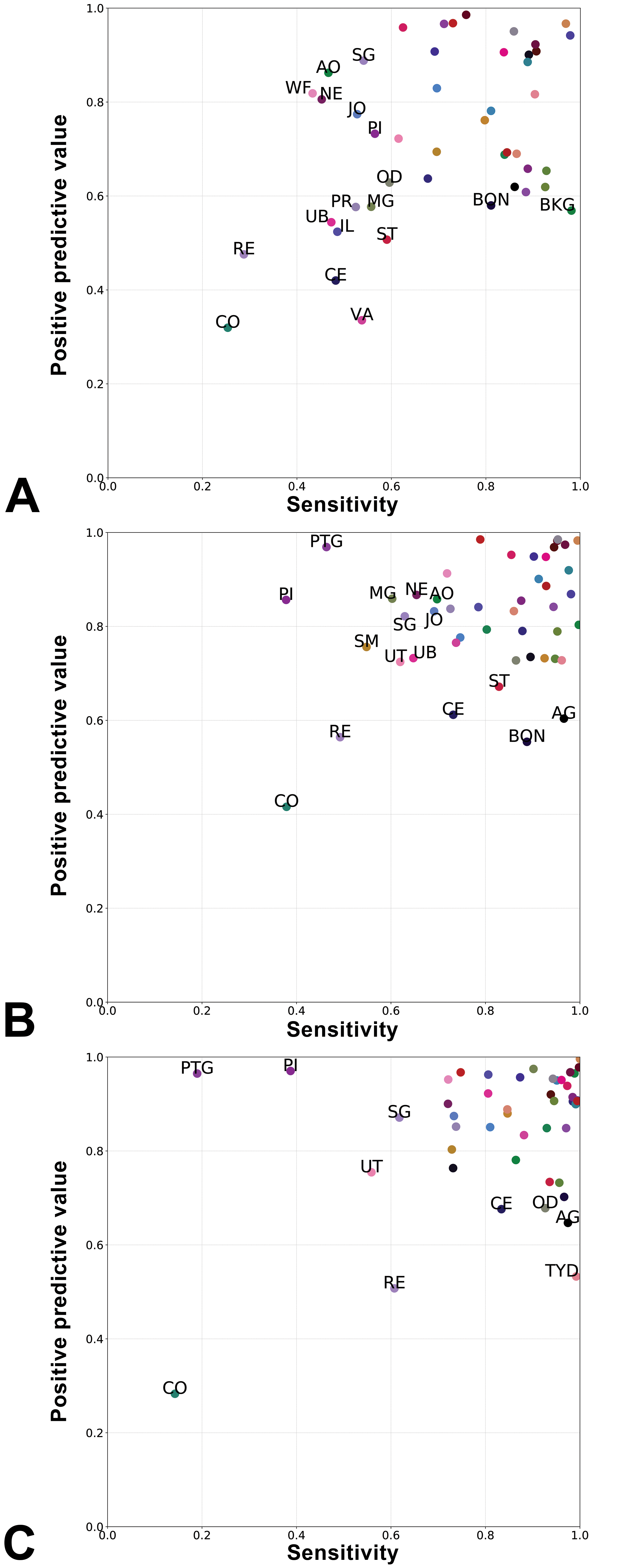
Positive predictive value and sensitivity of the Inception-v3–based models at 0.504 (A), 2.016 (B), and 8.064 mpp (C), for each tissue. Tissue class abbreviations (labels are shown only below a threshold of positive predictive value and sensitivity: 0.6 was used for 0.504 mpp, and 0.7 for 2.016 and 8.064 mpp). AG indicates adrenal gland; AO, aorta; BKG, background; BON, bone; CE, cecum; CO, colon; IL, ileum; JO, joint; MG, mammary gland; NE, nerve; OD, oviduct; PI, pituitary gland; PR, prostate; PTG, parathyroid gland; RE, rectum; SG, salivary gland; SM, skeletal muscle; ST, stomach; TYD, thyroid gland; UB, urinary bladder; UT, uterus; VA, vagina; WF, white fat.

Misclassifications were more frequent among histologically related tissues, where morphologies were shared at higher magnification (Supplementary Figures 1–3). Not surprisingly, regions of the large intestine (CE, CO, RE) and the small intestine (duodenum [DM], jejunum [JE], ileum [IL]) were often confused with each other, either as a single group (0.504 mpp) or as 2 groups corresponding to the midgut and hindgut (2.032 mpp). Similar confusions occurred between spinal cord (SPC), brain (BR), and nerve (NE), or joint (JO), bone (BON), and skeletal muscle (SM), or between thyroid (TYD) and parathyroid (PTG) (Supplementary Figures 1–3).

Analysis of Neural Network Embeddings

The embedding layer of the Inception-v3 network contains 2048 features. The exploration of such a high-dimensional space required dimensionality reduction using UMAP.²³ The UMAP was calculated exclusively using the embedding vector that is only from features learned by the model, without any information regarding the true class of the images. As models were trained for each magnification independently, a distinct projection of the embedding vectors for all test set patches was generated for each magnification (Figure 4A-E, left panel). The analysis of the embeddings was performed by pathologists reviewing the visual clusters together with images of the corresponding patches using a dedicated browser-based interface that had been created for this study.

Figure 4.

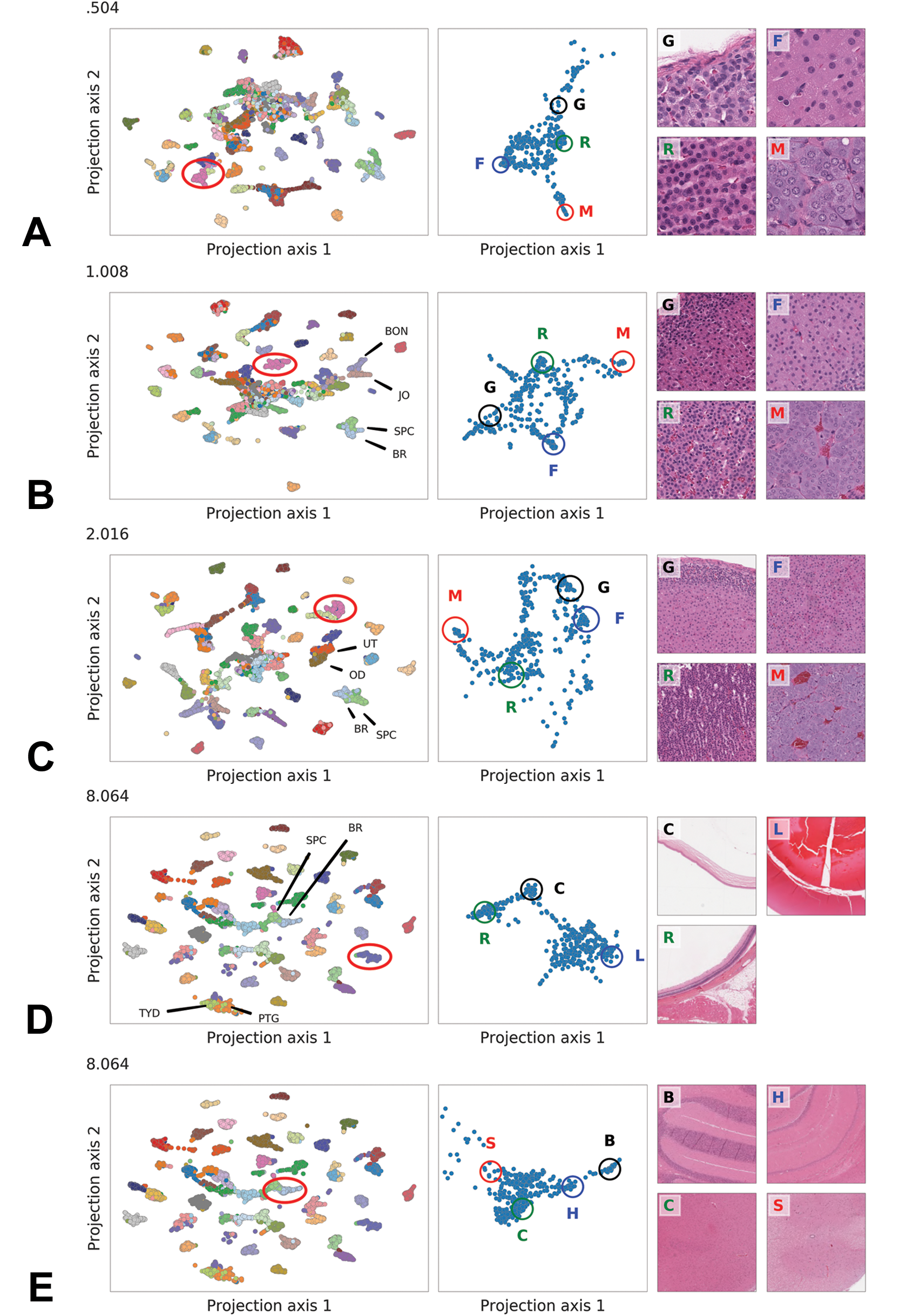
Uniform Manifold Approximation and Projection plots (left-hand column) of all rat test set tissues from low to high mpp (A. 0.504, B. 1.008, C. 2.016, D. 8.064, and E. 8.064), with a specific tissue cluster (circled) further represented in the clusters of the central column (A-C = adrenal gland, D = eye, and E = brain and spinal cord). Subanatomical sites are represented in each central column cluster and in the respective histological images of the right-hand column (adrenal gland: G = zona glomerulosa, F = zona fasciculata, R = zona reticularis, M = medulla; eye: R = retina, C = cornea, L = lens; brain and spinal cord: B = cerebellum, H = hippocampus, C = cerebral cortex, S = spinal cord).

Projections at all magnifications revealed groups corresponding to a large extent to true tissue classes. Groups were better separated at lower magnification (ie, higher mpp). Projections from models trained at high magnification showed a central aggregate of unresolvable patches, the size of which decreased with the resolution. Starting from 1.008 mpp, adjacent groups corresponded to tissue classes with similar morphology.

Many clusters of patches extracted from the same tissue were not compact when given a closer inspection and exhibited subclusters variably interconnected depending on the magnification at which the embeddings were generated (Figure 4A-E, middle panel). Visual inspection of the patches in these subclusters showed that they corresponded to histologically meaningful regions of the tissue. For example, patches representing the adrenal gland (AG) were clustered in subgroups showing different morphologies (Figure 4A-C, middle panel) that corresponded to distinct regions of the adrenal gland (AG), namely, the medulla and the cortex, and within the cortex to the zonae glomerulosa, fasciculata, and reticularis (Figure 4A-C, right panel). Similar histologically meaningful clustering was observed for the eye, where patches representing the retina, cornea, and lens were clearly separated from each other (Figure 4D), and for the brain (BR) (Figure 4E), with separation of the cerebellum, hippocampus, cerebral cortex, and the spinal cord (SPC).

The analysis of the embeddings also shed light onto magnification-dependent misclassifications between thyroid (TYD) and parathyroid (PTG), which are contiguous organs on rat histological sections. While at 0.504 mpp patches from TYD and PTG were well separated (Figure 5A), at 2.016 mpp the thyroid (TYD) and parathyroid (PTG) overlapped (Figure 5B). At 8.064 mpp, the parathyroid (PTG) represents only a small part of the patch (Figure 5C). Moreover, some thyroid (TYD) or parathyroid (PTG) patches containing skeletal muscle (SM) at low magnification clustered away from the glandular patches, closer to the skeletal muscle (SM) tissue group.

Figure 5.

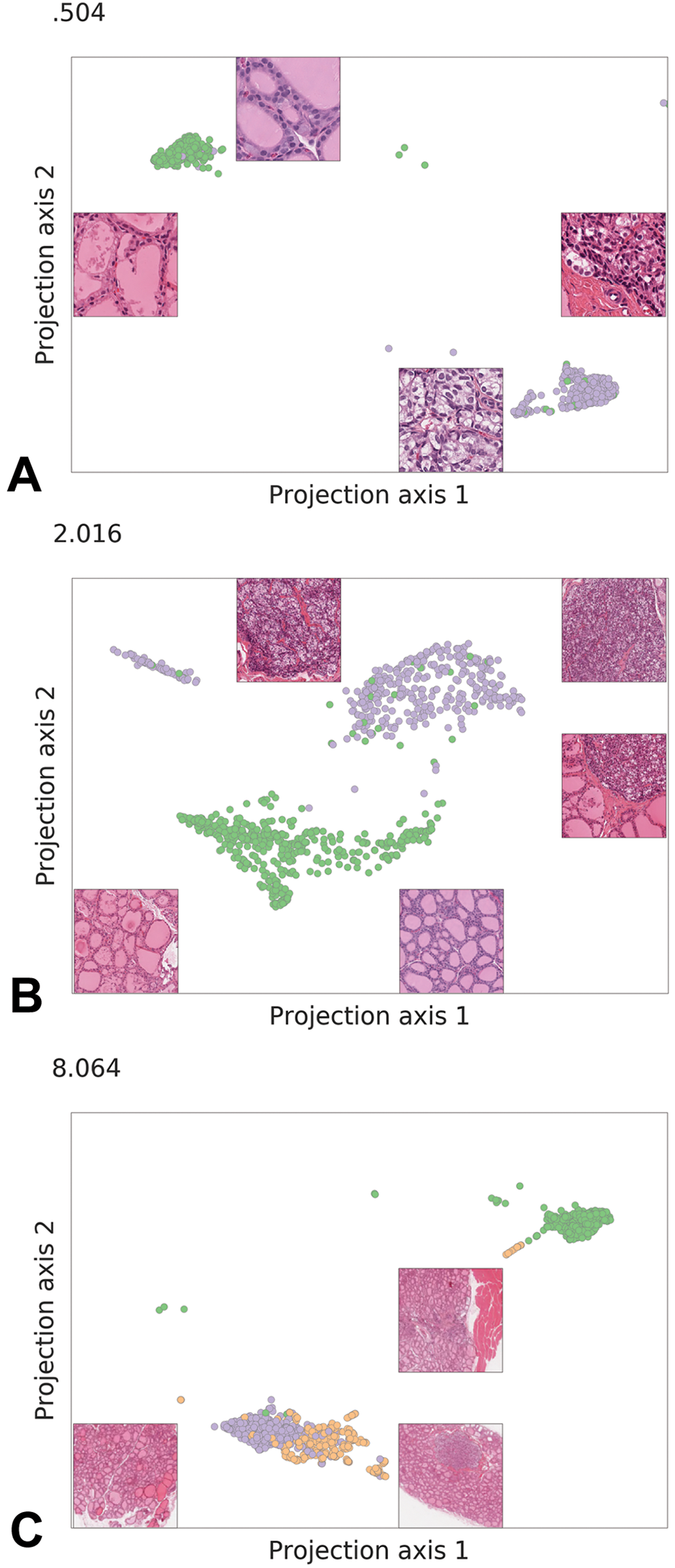
Uniform Manifold Approximation and Projection plots and respective histological images of thyroid and parathyroid gland at from low to high mpp levels (light blue: thyroid, mustard: parathyroid, red: skeletal muscle). At 0.504 mpp, patches from thyroid and parathyroid separate with only few exceptions (A). At 2.016 mpp, few patches occupy an intermediate position between the 2 main clusters (B). Such intermediate patches show fields comprising both thyroid and parathyroid tissues (mid-right). At 8.064 mpp, the cluster corresponding to thyroid and parathyroid blend into each other as with such large field of view most patch showing parathyroid tissue also contain a large proportion of thyroid follicles. In addition, some patches are projected in between the thyroid and the skeletal muscle corresponded to regions at the border of the organ where skeletal muscle is present (C).

Cross-Species Predictions and Transfer Learning

To assess generalizability, the Inception-v3–based rat model was then used—without any retraining—for cross-species prediction of independent data sets obtained from NHP and minipig covering 21 (NHP) and 36 (minipig) of the 46 tissues from the rat data set. All misclassifications were counted, no matter whether the error was due to a confusion among the tissues that were present in the NHP and minipig data sets or whether a tissue was predicted by mistake that only occurred in the original rat training data of 46 tissues from which the model had been trained. At 0.504 mpp, patch-level accuracy of the tissue predictions was 34.6% (NHP) and 39.3% (minipig). At 2.016 mpp, accuracy increased to 39.3% (NHP) and 45.2% (minipig). Finally, at 8.064 mpp, accuracy was 40.5% (NHP) and 42.0% (minipig). Many erroneous predictions corresponded to tissues that were absent from the NHP or minipig data sets (Supplementary Figures 4 and 5). Aside from these, confusions among histologically similar tissues, as observed with the rat data, were also present. Some tissues—brain, liver, kidney, thymus, spleen, lymph node, and thyroid—were recognizable at high accuracy in both NHP and minipig using the rat model, while other tissues—oesophagus, white fat, and tongue—were recognized well in only 1 species.

Given this relatively poor performance at cross-species classification without retraining, we next explored a scenario that allowed for retraining in order to adapt to a novel species. In particular, our goal was to assess whether the rat HistoNet model would be a better starting point for species adaptation than a generic ImageNet model. To this end, another independent study consisting of WSIs from 12 NHPs was used for training, while the NHP test set was the same as in the previous cross-species prediction without retraining. Two Inception-v3 networks were trained for each magnification: one initialized with ImageNet weights and one with the rat HistoNet weights. In addition, to determine the amount of training data necessary to achieve reasonable accuracy, a series of smaller training sets (using slides from 1, 2, 3, and 4 NHPs, respectively) was constructed from the full NHP training set of 12 animals.

Patch-level accuracies (Figure 6) were 85.8% (0.504 mpp), 92.4% (2.016 mpp), and 93.9% (8.064 mpp) when using the full training data set (N = 12 NHPs). These accuracies were substantially higher than those observed on the rat data set, as only 21 tissue classes were available for NHP, compared to the 46 tissue classes of the rat model, with some of the most difficult tissue classes missing.

Figure 6.

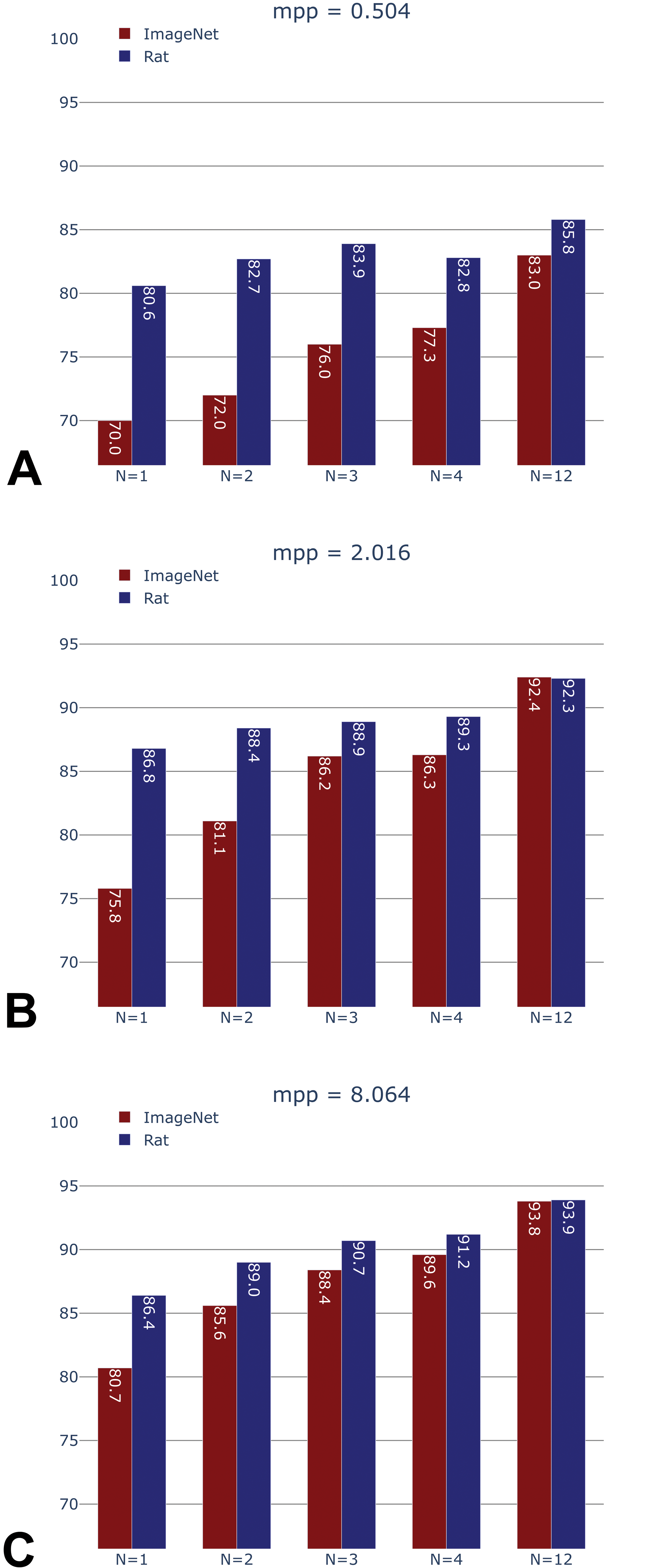
Non-human primate (NHP) test set accuracy of generic (ImageNet-pretrained) versus domain-specific (rat-pretrained) models, after training on N = 1, 2, 3, 4, and 12 (maximum available) NHPs, at 0.504, 2.016, and 8.064 mpp.

Importantly, when only limited NHP training data (1, 2, 3, or 4 NHPs) was made available, accuracies obtained by the NHP models initialized with the weights learned from the rat data set were consistently higher than those obtained with the standard initialization via ImageNet (Figure 6). For instance, the rat-initialized HistoNet model using samples from 2 NHPs attained an accuracy of 82.7% at 0.504 mpp, whereas this same accuracy was only reached for the ImageNet-initialized model when using the full data set of 12 NHPs (accuracy 83%). Likewise, at 2.016 mpp, the ImageNet-initialized network required samples from 4 NHPs in order to achieve the same performance as rat HistoNet with 1 NHP (86.3% vs 86.8%). The benefit of the rat-initialized models was less pronounced at 8.064 mpp, which is line with what was observed during the development of the rat HistoNet model.

Discussion

Tissue Recognition

We have shown that standard CNN architectures can be trained to recognize a comprehensive set of rat tissues at high accuracy across a broad range of magnifications. This even applied to some extent to subtle variations of histological structure, such as segments of the small (duodenum, jejunum, and ileum) and large (cecum, colon, and rectum) intestine, as well as to complex organs made of several tissue types (eg, eye or joint), for which small patches extracted at high magnification are typically difficult to classify by a pathologist in the absence of larger context. This suggests that a whole-tissue model could retain some specificity toward subtle histological features and therefore named HistoNet.

In general, tissue prediction was increasingly reliable with decreasing magnification. This can be easily understood given that a 224 × 224 pixel patch offers a narrow field of view (ie, exhibits only minimal context) at high magnification (56 × 56 µm at 0.252 mpp). With decreasing magnification, more structures are present on the patches, thus facilitating tissue recognition. However, small tissues such as the parathyroid represented an exception. Although it is recognized with consistently high PPV (meaning that if it is predicted, the prediction is usually correct) at all magnifications, the sensitivity decreased with decreasing magnification. In this case, widening the context is detrimental to the network’s recognition as other tissues occupy increasing amounts of space on a patch (for a visual example, see Figure 4C).

The majority of misclassifications were not due to unsystematic noise, but rather a result of confusions among histologically similar tissues. This was particularly prominent among segments of the large and small intestine, but also within the groups nerve, brain, and spinal cord and joint, bone, and skeletal muscle, respectively (Supplementary Figures 1–3). For the latter group, the confusion is likely due to joint as a tissue being subject to interpretation, with variable amounts of BON and skeletal muscle included in the manual outlines from which the patches are generated. Misclassification also occurred based on local histological similarity in some areas of the tissue regions such as between the periarteriolar lymphoid sheaths of the spleen and the cortex of lymph nodes (not shown). Finally, the confusion between the contiguous thyroid and parathyroid illustrated the role of magnification as discussed above.

For practical tissue-type classification, prediction on the level of large tissue regions would be more relevant than on individual patches. The performance at the region level across magnifications seemed at first counterintuitively constant compared to the patch level, the performance of which is highly magnification dependent. As mentioned above, this could be explained by the averaging out of nonsystematic errors at the patch level. Even if patches had only an accuracy of 50%, taking several of them combined and considering the majority prediction would result into a correct region identification.

Data Considerations

The development of HistoNet was made possible by the availability of large series of tissues from toxicology studies where systematic collection and processing of tissues ensure the highest histological quality. This sharply contrasts with classically used human specimens taken at autopsy the histological quality of which is usually poor due to autolysis. Notwithstanding dedicated efforts such as the GTEx tissue collection, autolysis is still an impediment, with several tissues (eg, pancreas, stomach, prostate) having a median grade of autolysis of 2.0 (data not shown). Moreover, unlike clinical surgical specimens often resected at an advanced stage of disease, a large proportion of samples from preclinical toxicology studies contain elementary lesions at various stages in relatively pure forms. This material offers a unique opportunity for the development of holistic histology and histopathology models.

A second data consideration is related to the substantial risks of overfitting (ie, representing the training set rather than the wider population) or inadvertently introducing an undesired bias via the composition of the training set: In earlier stages of this work, due to limited amounts of available data, the split into training and test sets had been performed on the level of animals rather than studies. Under these conditions, test set accuracies were substantially higher than those reported here. However, as we obtained data from additional rat studies, we found that the predictive performance on these new data sets was lower. This suggested that while stratified randomization on the animal level had prevented the network from overfitting to individual animals, it instead overfitted on the study level. One possible explanation for this could be the staining variations that persisted despite our stain augmentation. Furthermore, other possible explanations that are harder to mitigate are thickness of the section as well as the degree of contraction caused by the tissue fixation. In order to mitigate this effect, more studies were collected, and training and test sets were split by study.

Analysis of Neural Network Embeddings

A popular criticism against neural networks is that they are “black box” models, that is, harder to interpret than other machine learning methods. Although this criticism is valid, there are some techniques that shed light onto the nature of the model. As the learned weights and the neuron activations of CNNs are eminently visual concepts, a wide variety of methods for interpreting them have been suggested. In particular, the embedding vector, that is, the activations of the penultimate layer of a CNN, can be considered a mapping from a visual into a semantic space. Proximity in this space may be thought of as semantic, rather than purely visual similarity.

As shown above, the UMAP at all magnifications revealed clusters that correspond to a large extent to the true tissue classes. Adjacent or partially overlapping clusters often corresponded to tissues of similar morphology. Having pathologists studying the UMAP also aided in the interpretation of the apparent magnification-dependent confusion between thyroid and parathyroid.

Most strikingly, even though the annotations used for training the model only corresponded to coarse tissue/organ classes, the embedding layer learned by the network exhibited a degree of granularity that allowed for identifying histological substructures, which had found a distinct representation without prior annotation. This suggests that in order to differentiate tissues, the learned features focused on relevant tissue substructures. Therefore, although based on normal histology, our models could be applicable beyond the task it was defined for, such as in lesion detection or in content-based image retrieval.²²

Cross-Species Predictions and Transfer Learning

When applied to tissues from other species, the Inception-v3 models trained on rat showed high sensitivity and PPV only for some tissues. At the level of the individual tissues, it is interesting to note that those with very conserved structure such as liver, kidney, BR, TYD, and the lymphoid organs were classified with high accuracy across species. Not surprisingly, the gastrointestinal tract was often misclassified, which is not different from the prediction made on rat tissues.

Despite high predictive performance for some tissues, the rat model did not show sufficient overall accuracy on the cross-species prediction task to be immediately applicable. However, it provided a good basis for transfer learning to a novel species (NHP), superior to a model that had been initialized with ImageNet weights. The rat HistoNet model showed its biggest benefits when training data were scarce or the training task was hard (ie, at high-magnification levels). Of note, some of the tissues for which prediction was poor in the rat data set were not part of the NHP data set, which—along with the lower number of classes to predict (21 in NHP vs 46 in rat)—can explain the substantially higher accuracies seen in NHP, as compared to the original rat data.

In addition to being beneficial in the close-at-hand task of cross-species tissue classification, the approach of transfer learning from a domain-specific model described here may also be a suitable starting point when training for other tasks in the histology domain, for example, the recognition of a specific type of lesion for which only limited training data are available. In fact, this hypothesis is validated in another article contained in this special issue²² that shows, in a study on renal lesions, that the HistoNet pretrained model contains richer information for tasks such as biomarker classification, localization of biomarker-relevant morphology within a slide, as well as the prediction of expert-graded features compared to a model pretrained with ImageNet weights. In this article, Resnet-50 was used as the backbone of the model instead of Inception-v3. This reflects the very similar performance of these 2 architectures and the validity of either architecture as the basis for a HistoNet.

Related Work

Our suggestion of reusing domain-specific models relates to the notion of pretext tasks in machine learning,^24,25 in which a task is learned not (only) for its own sake, but to learn a feature representation that can be useful for other tasks in the same domain. Below, we discuss a few other topics that are relevant in the context of our work.

During the writing of this article, another study appeared, which also aimed at predicting tissue types from patches and, with a similar approach to ours however, with a focus on a software framework for reproducible machine learning.²⁶ Although this effort is in parts overlapping with our work, there are important differences between the 2 efforts. Our work focuses on several animal models (rat, NHP, minipig) instead of the human GTEx data set alone. For each animal model, we collected several independent studies and ensured that our training and test sets come from separate studies. As was discussed in detail above, these are crucially important features required for obtaining robust models and reliable (noninflated) performance estimates. In addition, we evaluate the effect of different magnification levels on the models. On the deep learning side, we train all our models end to end, including the convolutional feature generation layers, and we evaluate transfer learning between species. In the remaining paragraphs, we discuss further lines of related work.

Multiscale CNNs

The scanned slide images are of such high resolution that they contain diverse structural and textural information on different levels of magnification, from the level of individual nuclei to the level of entire tissues. Instead of training a separate HistoNet model for each magnification, as we have done in this work, an obvious extension would be to build a convolutional network that accepts such hierarchical input, that is, patches at several levels of magnification. This could potentially combine the benefits of having enough context on a patch with the advantages of lower magnification patches in recognizing smaller tissue structures, as was observed in an application of multiscale CNNs to high-content cellular images.²⁷

Visual explanations

In terms of interpreting the representations learned by the network, besides analyzing the embedding layer by means of nonlinear dimensionality reduction, a great number of approaches have been suggested that focus on different aspects of the model. One approach that will likely yield to greatly improved insight into what kind of structures or textural features are most relevant for a given class prediction is the Grad-CAM method.²⁸ Initial experiments with this technique for deriving “visual explanations” have been promising (data not shown).

Semantic segmentation and weakly supervised approaches

Besides our patch-based approach, several other machine learning paradigms have been applied to histopathology images. The most relevant of these are semantic segmentation using fully CNNs²⁹ and weakly supervised learning (multiple instance learning). The advantage of the latter approach is that unlike our approach or semantic segmentation, it does not rely on outlining structures within an image (which is often resource-intensive) but rather only requires a slide-level label. Weakly supervised learning is most applicable when large numbers of slides with reported findings are already available.⁹

Limitations

In this work, we have collected a substantial number of slides for training and testing, with 2 technically independent studies for testing. However, in future work, it would be desirable to have even more independent studies in order to cover a broader range of possible variation.

For the evaluation of cross-species predictions, we have used ImageNet-initialized models for comparison against our HistoNet-initialized models, as the former are widely used as a starting point in the imaging field and also in computational pathology.^30,31 Recent literature³² investigates the benefit of ImageNet versus randomly initialized models and smaller architectures in the context of medical imaging. Such an investigation for pathology images would be a possible topic for future research.

General Conclusion

This work was made possible by a continuous dialogue between data scientists and pathologists involved in annotations and interpretation of the UMAP. Our results show that it is possible to train models on the extensive diversity of tissue histology. Both the UMAP analysis and the cross-species transfer learning indicate that training on the coarse tissue annotations on one species yields embeddings that are much richer from a feature perspective than the original task would suggest. This is closely related to the concept of a pretext task, which is a useful form of reusing a learned representation when labeled data for a task of interest are scarce, but much more data are available that are either unlabeled or labeled for a different task.

Holistic histology classification models (HistoNets) such as those described here offer an advantage over ImageNet-initialized models for applications to histopathology: They open the perspective to generate numerical data from any histological picture or series of tiles from WSIs, creating general-purpose models for the classification of lesions and enabling content-based image retrieval and mining of morphological data in the histopathology domain. Furthermore, a tissue classifier as developed here could be part of an automated or semiautomated QC workflow in a laboratory.

Supplemental Material

Supplemental Material, sj-docx-1-tpx-10.1177_0192623321993425 - HistoNet: A Deep Learning-Based Model of Normal Histology

Supplemental Material, sj-docx-1-tpx-10.1177_0192623321993425 for HistoNet: A Deep Learning-Based Model of Normal Histology by Holger Hoefling, Tobias Sing, Imtiaz Hossain, Julie Boisclair, Arno Doelemeyer, Thierry Flandre, Alessandro Piaia, Vincent Romanet, Gianluca Santarossa, Chandrassegar Saravanan, Esther Sutter, Oliver Turner, Kuno Wuersch and Pierre Moulin in Toxicologic Pathology

Supplemental Material

Supplemental Material, sj-docx-2-tpx-10.1177_0192623321993425 - HistoNet: A Deep Learning-Based Model of Normal Histology

Supplemental Material, sj-docx-2-tpx-10.1177_0192623321993425 for HistoNet: A Deep Learning-Based Model of Normal Histology by Holger Hoefling, Tobias Sing, Imtiaz Hossain, Julie Boisclair, Arno Doelemeyer, Thierry Flandre, Alessandro Piaia, Vincent Romanet, Gianluca Santarossa, Chandrassegar Saravanan, Esther Sutter, Oliver Turner, Kuno Wuersch and Pierre Moulin in Toxicologic Pathology

Supplemental Material

Supplemental Material, sj-tif-1-tpx-10.1177_0192623321993425 - HistoNet: A Deep Learning-Based Model of Normal Histology

Supplemental Material, sj-tif-1-tpx-10.1177_0192623321993425 for HistoNet: A Deep Learning-Based Model of Normal Histology by Holger Hoefling, Tobias Sing, Imtiaz Hossain, Julie Boisclair, Arno Doelemeyer, Thierry Flandre, Alessandro Piaia, Vincent Romanet, Gianluca Santarossa, Chandrassegar Saravanan, Esther Sutter, Oliver Turner, Kuno Wuersch and Pierre Moulin in Toxicologic Pathology

Supplemental Material

Supplemental Material, sj-tif-2-tpx-10.1177_0192623321993425 - HistoNet: A Deep Learning-Based Model of Normal Histology

Supplemental Material, sj-tif-2-tpx-10.1177_0192623321993425 for HistoNet: A Deep Learning-Based Model of Normal Histology by Holger Hoefling, Tobias Sing, Imtiaz Hossain, Julie Boisclair, Arno Doelemeyer, Thierry Flandre, Alessandro Piaia, Vincent Romanet, Gianluca Santarossa, Chandrassegar Saravanan, Esther Sutter, Oliver Turner, Kuno Wuersch and Pierre Moulin in Toxicologic Pathology

Supplemental Material

Supplemental Material, sj-tif-3-tpx-10.1177_0192623321993425 - HistoNet: A Deep Learning-Based Model of Normal Histology

Supplemental Material, sj-tif-3-tpx-10.1177_0192623321993425 for HistoNet: A Deep Learning-Based Model of Normal Histology by Holger Hoefling, Tobias Sing, Imtiaz Hossain, Julie Boisclair, Arno Doelemeyer, Thierry Flandre, Alessandro Piaia, Vincent Romanet, Gianluca Santarossa, Chandrassegar Saravanan, Esther Sutter, Oliver Turner, Kuno Wuersch and Pierre Moulin in Toxicologic Pathology

Supplemental Material

Supplemental Material, sj-tif-4-tpx-10.1177_0192623321993425 - HistoNet: A Deep Learning-Based Model of Normal Histology

Supplemental Material, sj-tif-4-tpx-10.1177_0192623321993425 for HistoNet: A Deep Learning-Based Model of Normal Histology by Holger Hoefling, Tobias Sing, Imtiaz Hossain, Julie Boisclair, Arno Doelemeyer, Thierry Flandre, Alessandro Piaia, Vincent Romanet, Gianluca Santarossa, Chandrassegar Saravanan, Esther Sutter, Oliver Turner, Kuno Wuersch and Pierre Moulin in Toxicologic Pathology

Supplemental Material

Supplemental Material, sj-tif-5-tpx-10.1177_0192623321993425 - HistoNet: A Deep Learning-Based Model of Normal Histology

Supplemental Material, sj-tif-5-tpx-10.1177_0192623321993425 for HistoNet: A Deep Learning-Based Model of Normal Histology by Holger Hoefling, Tobias Sing, Imtiaz Hossain, Julie Boisclair, Arno Doelemeyer, Thierry Flandre, Alessandro Piaia, Vincent Romanet, Gianluca Santarossa, Chandrassegar Saravanan, Esther Sutter, Oliver Turner, Kuno Wuersch and Pierre Moulin in Toxicologic Pathology

Footnotes

Authors’ Note

Holger Hoefling, Tobias Sing, and Pierre Moulin contributed equally in this work.

Acknowledgments

The authors thank Geert Litjens for his helpful advice during the writing of this article.

Declaration of Conflicting Interests

All authors are employed by Novartis and hold shares in the company.

Funding

The author(s) received no financial support for the research, authorship, and/or publication of this article.

ORCID iDs

Tobias Sing

Imtiaz Hossain

Thierry Flandre

Oliver Turner

Pierre Moulin

Supplemental Material

Supplemental material for this article is available online.

References

Krizhevsky

Sutskever

Hinton

. ImageNet classification with deep convolutional neural networks. In: Pereira

Burges

CJC

Bottou

Weinberger

, eds. Advances in Neural Information Processing Systems 25. Curran Associates, Inc; 2012:1097–1105. Accessed June 4, 2019. http://papers.nips.cc/paper/4824-imagenet-classification-with-deep-convolutional-neural-networks.pdf

Esteva

Robicquet

Ramsundar

, et al. A guide to deep learning in healthcare. Nat Med. 2019;25(1):24–29. doi:10.1038/s41591-018-0316-z

Liu

Faes

Kale

, et al. A comparison of deep learning performance against health-care professionals in detecting diseases from medical imaging: a systematic review and meta-analysis. Lancet Digit Health. 2019;1(6):e271–e297. doi:10.1016/S2589-7500(19)30123-2

Hinton

. Deep learning—a technology with the potential to transform health care. JAMA. 2018;320(11):1101–1102. doi:10.1001/jama.2018.11100

Naylor

. On the prospects for a (deep) learning health care system. JAMA. 2018;320(11):1099–1100. doi:10.1001/jama.2018.11103

Louis

Gerber

Baron

, et al. Computational pathology: an emerging definition. Arch Pathol Lab Med. 2014;138(9):1133–1138. doi:10.5858/arpa.2014-0034-ED

Litjens

Kooi

Bejnordi

, et al. A survey on deep learning in medical image analysis. Med Image Anal. 2017;42:60–88. doi:10.1016/j.media.2017.07.005

Komura

Ishikawa

. Machine learning methods for histopathological image analysis. Comput Struct Biotechnol J. 2018;16:34–42. doi:10.1016/j.csbj.2018.01.001

Campanella

Hanna

Geneslaw

, et al. Clinical-grade computational pathology using weakly supervised deep learning on whole slide images. Nat Med. 2019;25(8):1301–1309. doi:10.1038/s41591-019-0508-1

10.

Madabhushi

Lee

. Image analysis and machine learning in digital pathology: challenges and opportunities. Med Image Anal. 2016;33:170–175. doi:10.1016/j.media.2016.06.037

11.

Bandi

Geessink

Manson

, et al. From detection of individual metastases to classification of lymph node status at the patient level: the CAMELYON17 challenge. IEEE Trans Med Imaging. 2019;38(2):550–560. doi:10.1109/TMI.2018.2867350

12.

Ehteshami Bejnordi

Veta

Johannes van Diest

, et al. Diagnostic assessment of deep learning algorithms for detection of lymph node metastases in women with breast cancer. JAMA. 2017;318(22):2199–2210. doi:10.1001/jama.2017.14585

13.

Veta

Heng

Stathonikos

, et al. Predicting breast tumor proliferation from whole-slide images: the TUPAC16 challenge. Med Image Anal. 2019;54:111–121. doi:10.1016/j.media.2019.02.012

14.

, et al. Computer-aided diagnosis of lung carcinoma using deep learning - a pilot study. ArXiv:1803.05471. 2018. [Cs], March. http://arxiv.org/abs/1803.05471.

15.

Coudray

Ocampo

Sakellaropoulos

, et al. Classification and mutation prediction from non–small cell lung cancer histopathology images using deep learning. Nat Med. 2018;24(10):1559–1567. doi:10.1038/s41591-018-0177-5

16.

Kather

Pearson

Halama

, et al. Deep learning can predict microsatellite instability directly from histology in gastrointestinal cancer. Nat Med. 2019;25(7):1054–1056. doi:10.1038/s41591-019-0462-y

17.

Janowczyk

Madabhushi

Deep learning for digital pathology image analysis: a comprehensive tutorial with selected use cases. J Pathol Inform. 2016;7(1):29. doi:10.4103/2153-3539.186902

18.

Tellez

Balkenhol

Otte-Holler

, et al. Whole-slide mitosis detection in H&E breast histology using PHH3 as a reference to train distilled stain-invariant convolutional networks. IEEE Trans Med Imaging. 2018;37(9):2126–2136. doi:10.1109/TMI.2018.2820199

19.

Simonyan

Zisserman

. Very deep convolutional networks for large-scale image recognition. In: International Conference on Learning Representations, October 28-29, 2021, Lisbon, Portugal; 2015.

20.

Szegedy

Vanhoucke

Ioffe

Shlens

Wojna

. Rethinking the inception architecture for computer vision. In: 2016 IEEE Conference on Computer Vision and Pattern Recognition (CVPR), June 27, 2016, to June 30, 2016. Las Vegas, NV, USA; 2016:2818–2826. doi:10.1109/CVPR.2016.308

21.

Zhang

Ren

Sun

. Deep residual learning for image recognition. In: 2016 IEEE Conference on Computer Vision and Pattern Recognition (CVPR), June 27, 2016, to June 30, 2016. Las Vegas, NV, USA; 2016:770–778. doi:10.1109/CVPR.2016.90

22.

Freyre

Spiegel

Gubser Keller

, et al. Biomarker-based classification and localization of renal lesions using learned representations of histology – a machine learning approach to histopathology. Toxicol Pathol. 2020;(Special Issue on Digital Pathology and Artificial Intelligence).

23.

McInnes

Healy

Saul

Großberger

. UMAP: Uniform manifold approximation and projection. Journal of Open Source Software. 2018;3(29): 861. https://doi.org/10.21105/joss.00861

24.

Noroozi

Favaro

. Unsupervised learning of visual representations by solving jigsaw puzzles. In: Leibe

Matas

Sebe

Welling

, eds. Computer Vision – ECCV 2016. Vol 9910. Springer International Publishing; 2016:69–84. doi:10.1007/978-3-319-46466-4_5

25.

Noroozi

Pirsiavash

Favaro

. 2017. Representation learning by learning to count. In 2017 IEEE International Conference on Computer Vision (ICCV), 5899–5907. https://doi.org/10.1109/ICCV.2017.628

26.

Bizzego

Bussola

Chierici

, et al. Evaluating reproducibility of AI algorithms in digital pathology with DAPPER. Rohde

, ed. PLoS Comput Biol. 2019;15(3): e1006269. doi:10.1371/journal.pcbi.1006269

27.

Godinez

Hossain

Lazic

Davies

Zhang

. A multi-scale convolutional neural network for phenotyping high-content cellular images. Bioinformatics. 2017;33(13):2010–2019. doi:10.1093/bioinformatics/btx069

28.

Selvaraju

Cogswell

Das

Vedantam

Parikh

Batra

. Grad-CAM: Visual explanations from deep networks via gradient-based localization. In 2017 IEEE International Conference on Computer Vision (ICCV), 2017:618–626. https://doi.org/10.1109/ICCV.2017.74

29.

Wang

Yang

Rong

Zhan

Xiao

. Pathology image analysis using segmentation deep learning algorithms. Am J Pathol. 2019;189(9):1686–1698. doi:10.1016/j.ajpath.2019.05.007

30.

Courtiol

Tramel

Sanselme

Wainrib

Classification and disease localization in histopathology using only global labels: a weakly-supervised approach. ArXiv180202212 Cs Stat. Published online February 20, 2020. Accessed October 5, 2020. http://arxiv.org/abs/1802.02212

31.

Hegde

Hipp

Liu

, et al. Similar image search for histopathology: SMILY. Npj Digit Med. 2019;2(1):1–9. doi:10.1038/s41746-019-0131-z

32.

Raghu

Zhang

Kleinberg

Bengio

. Transfusion: understanding transfer learning for medical imaging. In: Wallach

Larochelle

Beygelzimer

d’Alché-Buc

Fox

Garnett

, eds. Advances in Neural Information Processing Systems 32: Annual Conference on Neural Information Processing Systems 2019, NeurIPS 2019, December8-14, 2019, Vancouver, BC, Canada ; 2019:3342–3352. Accessed Novembre 30, 2020. http://papers.nips.cc/paper/8596-transfusion-understanding-transfer-learning-for-medical-imaging

Supplementary Material

Please find the following supplemental material available below.

For Open Access articles published under a Creative Commons License, all supplemental material carries the same license as the article it is associated with.

For non-Open Access articles published, all supplemental material carries a non-exclusive license, and permission requests for re-use of supplemental material or any part of supplemental material shall be sent directly to the copyright owner as specified in the copyright notice associated with the article.

0.00 MB

0.01 MB

0.02 MB

0.27 MB

0.23 MB

0.22 MB

0.24 MB

0.91 MB