
Abstract
It is a common problem to distinguish a minor treatment change from background variation, especially when establishing no observed effect levels. Toxicological histopathologists use a wide range of methods at the microscope for comparing groups to help them form their opinions. Although the data produced by these methods can be subjective, all of these methods produce data that can be formally analyzed to give an objective, probabilistic result, provided the observations are unbiased. Other important experimental disciplines make extensive use of completely subjective data to produce objective results, for example, clinical trials using patients' symptoms. It is argued here that pathological experimental data too should be analyzed before an expert opinion (along with the objective evidence for that opinion) is formally reported. The Ordering Method, based on ranking the severity of a putative toxic change, is the most sensitive, robust, and analytically flexible method currently available.
Introduction
It is a common dilemma for histopathologists at the bench to see a small difference between treated and control groups and to be unsure if that difference is just a chance distribution of a naturally variable feature or a genuine treatment-related effect. This is particularly acute when setting no observed effect levels (NOELs), where very fine histological distinctions at the very margins of experimental sensitivity can have large implications for safety margin calculations (and hence compound development). The objective of this review is to show that when unbiased histopathological data are judiciously gathered at the microscope, they can be rationally analyzed to give meaningful, objective results that can be judged against accepted scientific norms (such as the 95% confidence limit). If an experiment is run, the data are gathered, and only at this late stage a method to analyze them is sought, then the chances of the experiment actually giving any result are diminished. How data are to be analyzed should determine the nature of the data to be gathered, rather than the reverse. So this article will concentrate less on the examination of the slides or diagnostic criteria and more on the nature of the observations required that allows a subsequent objective analysis. The method to be adopted at the microscope then follows naturally from the nature of the observations desired. An example of the issues addressed would be, Is scoring lesions (mild, moderate, marked) the best way to collect data for analysis, or should one record the animals in the order of the severity of any lesion? We wish to raise such issues for more widespread discussion with this article.
Although almost all toxicologic histopathological data are subjective, this does not mean that they cannot be gathered without bias, be analyzed, and then have firm probabilistic inferences and objective conclusions based on them. For many decades, patients' subjective symptoms and opinions of their treatment have been gathered in clinical trials. Firm objective results with probability estimates are obtained from the mathematical analysis of these subjective views. A textbook example would be McLean and Hakstian (1979), where the subjective symptoms of depressed patients after their talking, behavioral, and drug treatments were objectively compared—note that this example was chosen by statisticians for a statistics textbook (Siegel and Castellan 1988, Example 8.1a,b). If clinicians can get objective results from the subjective opinions of patients, it should be possible to get objective results from the subjective opinions of well-trained, mentally healthy professionals working under laboratory conditions.
Some nonroutine histopathology data, such as image analysis data, are gathered in an unbiased form and routinely subjected to analysis. Such data are usually numeric, from which parameters such as mean and standard deviation can be meaningfully obtained. This allows the common parametric statistical techniques to be used on them. The opinion-based results of a visual examination cannot be presented as meaningful parametric numeric data, so any objective analysis can only be conducted using nonparametric techniques. This is the approach taken here.
All of the methods given below come originally from pathologists working in toxicological histopathology—some to many toxicological pathologists are using each of these methods on their day-to-day study material. Each method has at least some advocates who commonly use them (see the raw data given in Holland 1996); none are new. It must be granted that most users do not then push their method to the logical conclusion of the statistical analyses advocated here. However, if an experimenter produces data suitable for formal analysis and then does not do and use that analysis in the interpretation of his or her data, he or she may not achieve objective results and conclusions.
Unless you have asked numerous colleagues to explain in detail how they actually distinguish small real effects from background variations, some of the techniques they employ may be a surprise and very counterintuitive to you. In Figure 1 , a small data set is given, and then it is explained how pathologists who use each method prepare the data, what information they extract, and how they use it to decide whether the difference in the data is real or just a chance event. If the detailed descriptions in the body of the text appear confused or pointless, refer to the concrete examples of each method in Figure 1 to give you insight into each method’s rationale.
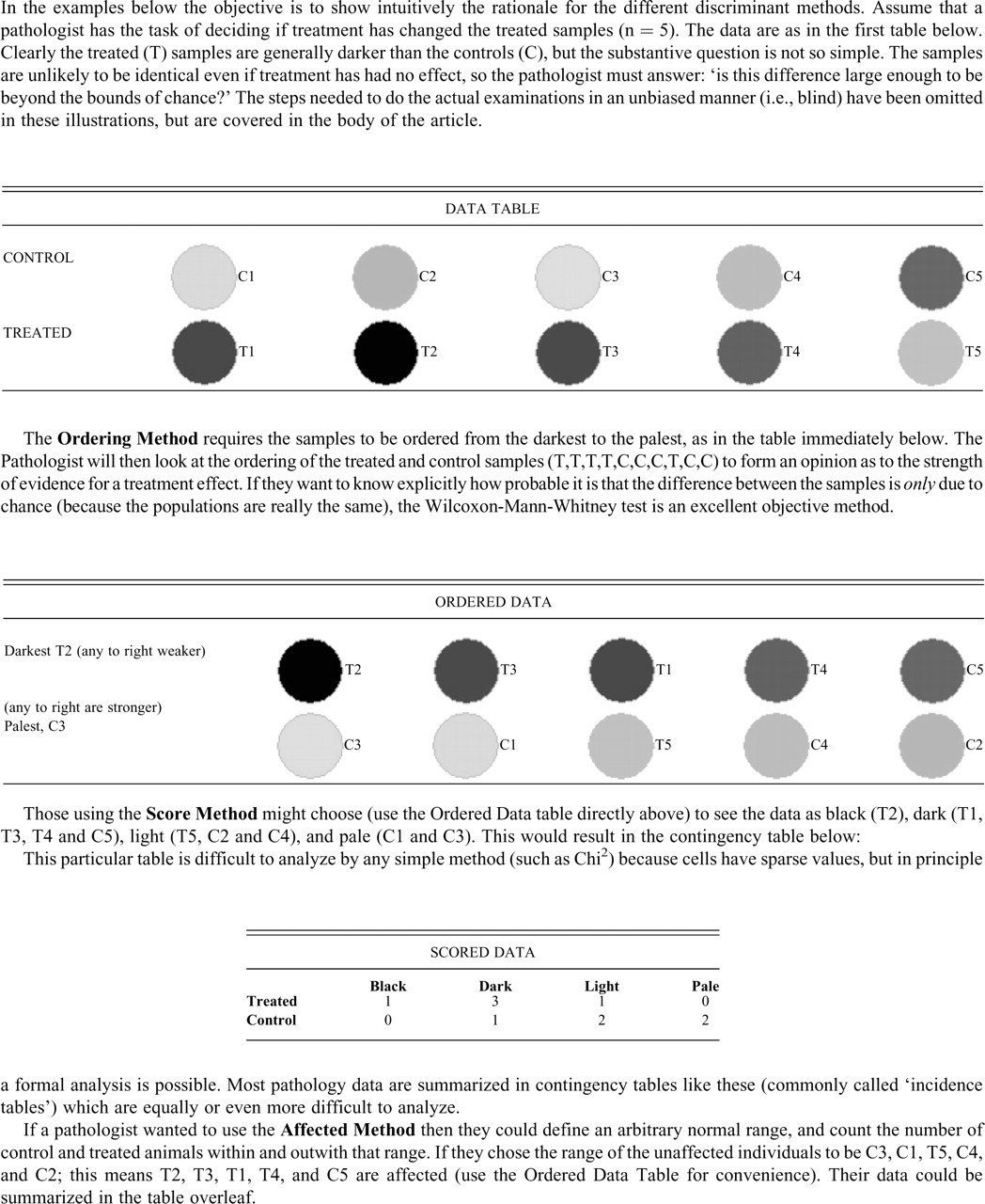
Illustrations of the practical application of the discriminant methods.
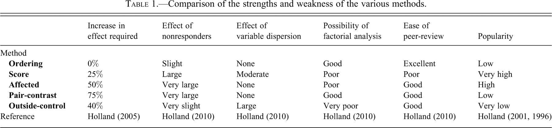
The comments on the relative strengths and weaknesses of the various methods are based on data and analyses drawn from some arcane techniques. These techniques, and the detailed results from them, have already been published in the peer-reviewed literature (Holland 1996, 2001, 2005, 2010). The intention in this article is to point out the practical consequences of these earlier results. Those interested can go to these original references to see the detailed data that support these recommendations.
The sensitivity of the various methods is compared in these terms: the size of treatment effect for the method under discussion to just achieve 80% power has been measured (this is a conventional target for sensitivity, meaning that if an experiment were run 100 times with the same or a certain difference between the groups at the same confidence level, then it would detect the difference 80 times [Holland 2010]). This size of effect that achieves 80% power for each method is compared with the size of treatment effect needed to be detectable with 80% power by the most powerful of the techniques (in this case the Ordering Method using a Wilcoxon-Mann-Whitney test [WMW]) at the same power [Holland 2010]). The result is given numerically as a percentage increase—so a method that achieves 80% power only when there is twice the difference between the groups required for the Ordering Method to achieve this power is described as requiring a 100% increase in effect compared with the Ordering Method.
Assumptions
The following are assumed: Two groups of 10 animals need to be compared to see if a real difference between them exists—so this article covers typical rodent studies but not large animal studies, with group sizes of 3 or 4, nor carcinogenicity studies. The difference (or lack of it) needs to be expressed in objective terms, even if the data themselves are subjective. The feature of interest is known before the unbiased examination takes place, so there is no need to find the difference between the groups during the examination. This requires a prior examination of the material to identify what is putatively related to treatment and what is not. There are no features other than the one of interest that could indicate from which group an individual comes. The slides can be randomized and examined blind to treatment, group, or findings in other organs, without the histopathologist being able to recall to which group any individual belongs (if she or he did the initial examination to identify features of interest, for example). The final assumption is that a toxic effect is only a change in one direction and that a change in the opposite direction is innocuous (so increased hepatic bile pigment is an indication of toxicity, but a treatment-related decrease in bile pigment is not an indication of toxicity). In technical terms, these are simple alternative hypotheses that would be tested with a one-tailed test. In some organs, this clearly cannot hold—both increased and decreased cellularity in lymphoid organs can be regarded as indications of toxicity. However, extending the idea from simple one-sided testing to composite hypothesis two-tailed testing follows naturally from the work outlined here.
Methods
Ordering Method
In this method, the pathologist places the slides in order from those showing the most extreme form of the feature of interest to the least (or the least to the most affected, which is an equivalent procedure). The slides need to be placed in rank order (see Figure 1 for an illustration). So if one were interested in centrilobular hepatocellular hypertrophy as a possible treatment effect, one would find the individual with the most prominently hypertrophied lobules, then the second most prominently affected individual, the third, and so on to the least affected.
There are a variety of approaches at the microscope to achieving this ordering. Traditionally a bubble-sort always works. A simple way of performing a bubble-sort is Go through the slides and find the most extreme example of the lesion of interest. Put the most extreme example found in step 1 aside from further examination. Repeat steps 1 and 2 with remaining slides. Stop when all the slides have been put aside.
The order in which slides are put aside is the order (or rank) of the severity of the feature of interest. This is laborious; it is quicker and easier to roughly sort the slides into order and then go through in detail, ensuring that each individual shows less of the feature of interest than the previous slide, until an examination of all of the material in order requires no changes.
If possible, assigning two or more animals to the same rank should be avoided. Where there are a few ties, then the subsequent analysis is not substantially affected, but to have many ties reduces the method to a disorganized and suboptimal scoring system (Siegel and Castellan 1988). There is one common situation where ties are inevitable—some animals do not show the feature of interest at all. This is part of a wider problem with many tests—the presence of nonresponders can very substantially affect, and even totally abolish, a method’s power.
The Ordering Method is not popular (Holland 2001, 2005) but has many strengths, which spring from the analyses that can be done on data of this sort. Ordered data can be analyzed for a treatment effect using the WMW test. If the feature is consistently normally distributed, then the WMW test achieves almost the maximal theoretical discriminant power possible. The WMW test is robust if the groups differ in their variances, in that it remains sensitive to changes in location only, rather than detecting change in variance and change in location. If there is a treatment effect, but some individuals of the treated group are nonresponders, the WMW test retains some power but it is substantially reduced.
One of the greatest strengths of the Ordering Method is the range and versatility of the tests that can be applied to ordered data. The WMW test can be usefully extended. It requires a firm grasp of statistical theory to include both sex and treatment in a factorial WMW analysis, although it can be easily implemented. The test can be extended to a trend test for dose (the Jonckheere-Terpstra test, or JT [Conover 1999]), which itself can also be extended to include sex as a factor in the analysis. All of the family of tests based on the Kolmogorov-Smirnov test can be applied to ordered data (Conover 1971); Shirley’s test to establish a NOEL would be applicable when the data extend to more than one dosed group (Williams 1986).
The method is easy to implement blind to all other data from the study. At the microscope, ordering 20 slides from most to least affected is a simple task (a task of about 2 hours). It would be explosively onerous with much larger numbers (for example, 80 animals for a full JT test in two sexes). Diagnostic drift is not a problem, because a final check that the ordering is correct does not involve remembering any arbitrary severity bands, just a check that the last slide that was examined was less or more extreme (depending on the direction of the check) than the current one. Review of others' work is easy; take the most extreme and third most extreme and confirm they are in the correct order, then the second and fourth, and repeat this process exhaustively. If there are no discrepancies, then the reviewer can only disagree with adjacent ranks, which is trivial.
Score Method
In this method, the severity of the lesion of interest is divided into ordinal classes (scores or grades, e.g., minimal, mild, moderate, marked). See Figure 1 for an illustration of the method. The more classes there are, the more sensitive the method becomes—ultimately becoming as sensitive as the Ordering Method when the number of classes equals the number of samples. Less intuitively obvious is that the sensitivity of the method is maximized for a given number of classes by having uniform class sizes. Many people feel unhappy with the allocation of class boundaries to give equal class sizes—they quite naturally feel that extreme examples of a lesion are rare, so they tend to have large classes in the center of the range and small classes at the two extremes. This reduces the power of the method.
Analysis of the sparse contingency table that results can be difficult. If the expected class sizes are not small, then a simple chi-square test is adequate. Exact tests and tests based on simulations are available in specialist statistical packages (StatXact and SAS), and the data may be suitable for generalized linear regression models such as logistic regression.
Comparison of the strengths and weakness of the various methods.
The Score Method is overwhelmingly the most popular method used (Holland 1996, 2001) and regarded as sensitive by a large majority of pathologists. In fact, it is less sensitive than the Ordering Method—there needs to be about a 25% increase in the severity of lesions over that which an Ordering examination will reliably detect before Scoring will also detect it (Holland 2010).
Score data have further substantial disadvantages (Holland 2010). This test for difference in location also detects differences in dispersion (e.g., treatment just makes the population under treatment more variable in a feature rather than consistently increasing or decreasing that feature). So a positive result is ambiguous and means that, unless it can be shown that the variances are not different, it is never known what confidence level any result had actually achieved. Conceivably, a reduction in dispersion could even hide a change in location. It is difficult to make a factorial analysis (using sex and treatment as factors) with sparse contingency tables (although it can be done and is exactly what is achieved in the Peto test, using tumor, death class, and time period as factors). If there are nonresponders in the treated group, the method’s sensitivity is substantially reduced.
At the microscope, score data are easy to gather blinded to animal and to treatment. Because the boundaries between the classes are subjective and arbitrary, it is difficult to eliminate diagnostic drift and impossible to define how a table was generated, so that a peer review is difficult. It can be very difficult for the original pathologist to re-create the table after a short interval of time. If it is necessary to check rigorously a given table, the reviewer either has to go through each animal, comparing it with all those in the grades above and below, or rank all the slides and individually check each animal in the ranking against all the others for inconsistency with the tabulated values. In practice, one regenerates a table using one’s own class boundaries and assesses if it generally fits with the original.
Affected Method
In this method, the experimenter decides the range of the normal, examines all the slides blind to animal and treatment, and then picks out those individuals outside this range (this is illustrated in Figure 1). The normal range can be taken from personal preference, expert opinion, historic material, or any other source. If the concurrent controls are used to define “normal,” then this becomes the Outside-Control Method (see below). The data are a 2 × 2 contingency table of affected and unaffected by control and treated. To maximize sensitivity, all the marginal subtotals should be identical, and the further one moves from this restriction, the more power is being sacrificed.
A Fisher’s exact test is the most powerful way of analyzing data in this form (Sprent and Smeeton 2007).
While this method is popular (Holland 2001, 2005) it is substantially insensitive—it requires the lesions to be 50% more extreme in the treated groups than that which an Ordering Method will detect reliably. If a less dispersed distribution is present (such as the uniform), this deteriorates so that a 70% increase over that required to achieve a significant result to the Ordering Method is needed, but it is as sensitive as the Ordering Method with more dispersed distributions (such as the exponential distribution [Holland 2010]). It is unaffected by the variances of the populations being different. The presence of a significant number of nonresponders in the treated group completely obliterates any ability of this test to detect an effect of any magnitude.
At the microscope, this is a very easy way to gather and check data blind. Although it might appear to be affected by diagnostic drift, it is so simple to review (simply find the most developed unaffected and the least developed affected and compare them) that in practice this is never a problem.
Pair-Contrast Method
This method compares individuals from each group in pairs to find if there is a consistent difference between the groups. So a practical procedure would involve pairing each control sample with a treated sample—giving 10 pairs. The lesion of interest in each member of a pair is compared (blind as to which group they come from) and the most affected noted, until all the pairs have been assessed. The result after breaking the code is the number of pairs in which the control is the more affected and the number of pairs in which the treated is the more affected (see Figure 1).
The Sign test is the standard test for data of this type (Siegel and Castellan 1988).
If this test is applied at the conventional 95% confidence limit (this means in 9 or 10 of the comparisons the treated sample was the more extreme—in reality, this is the exact 98.9% confidence limit), then this is a very insensitive method. It requires a change 75% larger than that required by the Ordering Method. It is stable in the face of differing variance between the groups, but if there is even a small number of nonresponders in the treated groups, the method fails to detect any magnitude of treatment change.
In practical terms, it is very easy to implement blind at the microscope, requiring probably the minimum effort of all the methods (10 comparisons). It is very easy to review. It is unaffected by diagnostic drift. There is the possibility of a factorial analysis with this method. It is the least popular method (Holland 2001).
This method can be applied at the 94% confidence limit by taking 8, 9, or 10 comparisons out of 10 having the treated sample as the more extreme as significant (limiting a significant result to only 9 or 10 comparisons to exceed the 95% confidence limit makes this a very conservative test). There is no special reason for specifying the 95% confidence limit as the arbitrary portal of a significant result; 94% is just as reasonable. This change substantially affects the power of the Pair-Contrast Method—it then becomes more powerful than the Score Method and only slightly less powerful than an Ordering Method. Its other strengths and weaknesses are unaffected by this change.
Outside-Control Method
This method involves counting the number of animals in the treated group that are outside the range of the concurrent controls (see Figure 1 for an illustration). The authors are only aware of its ever being implemented thus: find the most extreme control sample by going through all the controls, and then compare this single control sample to all the treated samples and count how many of the treated group are more extreme than this most extreme control. This implementation is clearly subject to observer bias, as the observer always knows to which group the material under the microscope belongs.
However, it would be easy to adequately blind this method to group and animal by several different examination techniques. For example, blind rank all the samples (as for the Ordering Method) and simply count the number in the treated group outside the range of the controls. A substantially less labor-intensive method would be to bubble-sort the most extreme individual, break the randomization code for this individual, and then repeat this process with the remaining randomized samples until the most extreme control is found. The number of rounds of the bubble-sort, less one, is then the number of treated animals outside the range of the controls.
There are no published standard statistical tests for data of this sort, partly because it is easy to work out the exact probability of getting any particular result under the null hypothesis from first principles. For those with a background in probability: the total number of all possible orderings is 20C10 and the total number of orderings with n individuals in one specified group as more extreme than any individuals in the other group is 20-nC10-n . Assuming there is no difference between the groups (the null hypothesis), any of these orderings is equally as likely as any other. So, the probability of getting a distribution with n (or more) individuals from a specified group outside the range of the other group in the direction required is the quotient of these two combinations. This probability is the exact p value of getting n treated animals outside the range of the controls. Numerous other methods will also give an exact result.
The Outside-Control Method is neither a popular nor a sensitive method. It requires an increase of effect of some 40% over the Ordering Method to achieve the same power (Holland 2010). The authors are unaware of any discriminant test of this form used outside toxicological pathology. It has obvious weaknesses that are probably the reasons no recognized statistical test is based upon it. All the information about the control group is summarized in the most extreme control animal. It is impossible to choose a worse representative to encapsulate the information in the control group than the most extreme example. Choosing the third most extreme or median animal at least avoids the possibility of using a method that will automatically select an anomalous outlier to represent the control group (and hardly complicates the statistical arithmetic). Although its sensitivity appears poor (requiring a 40% increase in effect compared to the Ordering Method), this flatters the method because it was calculated using the conditions under which the test is valid (i.e., without including outliers). A better view would be that even when there are no outliers (which the method will select whenever they occur in the controls and reduce the method’s sensitivity), it is still an insensitive method. It has a further, more subtle weakness. It is usually used by taking the number of treated animals that exceed the most extreme control animal as the test value. However, the same reasoning could lead to taking the number of control animals that fall below the range of the treated animals as the test value. A single data set could then be both significant and nonsignificant to the same test (which is the case in Figure 1).
However, it has one feature that makes it of particular interest. Unlike all the other methods, even if half of the treated group is nonresponders, then its sensitivity is only slightly affected (Holland 2010). Furthermore, the Outside-Control Method can be applied to the data gathered for the Ordering Method without any extra work at the microscope; it can be obtained directly from the ordering needed for the Ordering Method. So it can be used to check the only weakness in the Ordering Method: that nonresponders reduce the sensitivity of the Ordering Method. If the data gathered for the Ordering Method shows no clear effect itself, but the most extreme 4 or more of the animals belong to the treated group, then this suggests a treatment effect is present, but hidden from the WMW test by nonresponders in the treated group.
Discussion
It must be stressed that it is only reasonable to use the analytical methods given above if the data are unbiased. This means the data must be gathered with the observer completely blind to the individual’s treatment (among other conditions). There is no need to formally analyze data that has been gathered with knowledge of the treatment group. No amount of intricate statistical theory or manipulation can separate the real differences that exist from any differences that may only exist in the mind of the observer in potentially biased data.
Observations of an informed observer can validly be used to support an expert opinion. But such an expert opinion is just that: an opinion. In contrast, a credible experimental finding is the culmination of a valid method, unbiased data, and an objective analysis that gives rise to a unique conclusion. An experimental result, based on objective analysis of unbiased experimental evidence, is currently the closest to true knowledge that the scientific method can achieve. The objective analysis of unbiased data are an essential part of this process. These steps are usually absent from pathology reports.
The Ordering Method has overwhelming advantages compared to all other methods. It has the greatest power, is easily extended to all dose groups for a trend test, and can be run in a factorial manner to include sex as a factor in the experimental design. There are a wide range of tests that can be run on ordered data to answer specific hypotheses. It is one of the least affected methods when some of the treated animals fail to respond, when it can be combined with the Outside-Control Method to detect that situation. It is easy to review.
In contrast, the Score Method data are less sensitive and more difficult to review than the Ordering Method; it detects both change in location and variability (which frustrates interpretation of any positive outcomes), loses power with nonresponders, and is very difficult to analyze in a factorial manner. The Outside-Control, Affected, and Pair-Contrast Methods are much less sensitive than the other methods, although if the Pair-Contrast Method is applied at the 94% confidence limit, it has more power than the Score Method. The Affected and Pair-Contrast Methods lose all ability to detect any size of treatment effect if there are numerous nonresponders. However, any objective method applied to unbiased data is preferable to a simple subjective opinion drawn from potentially biased data. We hope that this article will stimulate a critical discussion on these important issues.
Footnotes
Acknowledgments
This work is drawn from a Fellowship Thesis of the Royal College of Veterinary Surgeons (![]() ). Tom Holland owes a great debt to his two supervisors, Mr. Peter Lee and Dr. John Glaister. We gratefully thank Dr. Annabelle Heier and Dr. A. Peter Hall for constructive criticism of the text and Prof. John Foster for his encouragement and help with the article.
). Tom Holland owes a great debt to his two supervisors, Mr. Peter Lee and Dr. John Glaister. We gratefully thank Dr. Annabelle Heier and Dr. A. Peter Hall for constructive criticism of the text and Prof. John Foster for his encouragement and help with the article.
The author(s) declared no potential conflicts of interest with respect to the authorship and/or publication of this article. The author(s) received no financial support for the research and/or authorship of this article.