
Abstract
This study develops and solves a micropolar-fluid model for heat storage in a rectangular duct subject to constant wall heat flux. The dimensionless mass, linear and angular momentum, and energy equations are treated with a Runge-Kutta (for the coupled momentum ODEs) and finite-difference scheme (for the energy PDE). Increasing the coupling parameter raises the dimensionless axial velocity while initially reducing and then increasing microrotation; the net effect is a decrease in dimensionless temperature, indicating diminished storage effectiveness. In contrast, higher spin-gradient viscosity reverses these trends and enhances thermal storage. Reynolds and Prandtl numbers exhibit inverse relationships with the temperature profile. Quantitatively, the mean Nusselt number is
Introduction
As global energy needs grow, demand for energy services rises, driving a shift to renewable energy, particularly solar, in response to climate change and declining traditional resources. Fossil fuel use has increased emissions, environmental issues, geopolitical tensions, and fuel prices. These challenges pose significant threats to society, making sustainable energy sources essential (Asfar et al., 2023; Khan et al., 2025). Countries are shifting to clean energy, with solar power being the key to its abundance and sustainability (Al-Ghussain et al., 2025). Technological advances and lower costs have made solar energy a vital renewable resource for electricity and water heating. Switching to solar energy benefits the environment, economy, and creates jobs, while driving growth, innovation, and technological progress (Alrbai et al., 2023, 2022).
Solar energy faces challenges such as interruptions caused by sunlight variations and weather changes. These fluctuations affect its reliability, especially for sectors requiring a continuous power supply (Shutaywi et al., 2024). Effective storage systems are therefore essential to store excess energy during peak sunlight and supply it during low-radiation periods (Khan et al., 2024a; Shutaywi et al., 2025). Thermal energy storage (TES) allows short-term retention of thermal energy at varying temperatures, contributing significantly to energy savings and enabling low-cost thermal energy and power generation (Khan et al., 2024b; Raza et al., 2024a). Its importance has grown in addressing supply–demand mismatches in intermittent renewable energy (Khan et al., 2023b; Raza et al., 2024b). Well-designed TES systems minimize thermal losses while maximizing energy extraction efficiency. TES technologies include sensible heat storage, latent heat storage using phase change materials (PCMs), and thermochemical storage (Raza et al., 2024b; Raza and Ashfaq, 2025). TES plays a crucial role in applications such as concentrated solar power and HVAC systems, with recent advancements highlighting its potential to transform energy technologies (Khan et al., 2023c; Rathore et al., 2025). Among solar thermal systems, water heating is widely adopted worldwide, reducing reliance on fossil fuels and greenhouse gas emissions (Khan et al., 2022; Kumar et al., 2025). Evacuated tube collectors (ETCs) achieve higher efficiencies than flat-plate collectors (FPCs) by employing vacuum insulation to minimize conduction and convection heat losses (Anantha Kumar et al., 2023; Kumar et al., 2019). ETCs can absorb up to 80% of solar energy compared to about 60% for FPCs, making them suitable for both heating and cooling applications. Their wide operating temperature range (–30 to 130 °C) enhances durability and reduces maintenance needs (Anantha Kumar, 2024; Anantha Kumar et al., 2025).
In addition to collector design, the choice of working fluid plays a central role in enhancing the efficiency of thermal energy storage systems. Micropolar fluids extend the classical Navier–Stokes framework by incorporating the effects of microrotation and microstructural interactions within the fluid (Khan et al., 2023d; Ramadevi et al., 2020). Unlike Newtonian fluids, which assume constant viscosity and neglect particle-scale effects, micropolar fluids account for the presence of rigid or semi-rigid microelements suspended in the medium (Khan et al., 2023a; Ramadevi et al., 2019a). These particles generate asymmetric stress tensors and additional rotational degrees of freedom, which fundamentally modify the flow and thermal transport characteristics (Ramadevi et al., 2019b). As a result, micropolar fluids can exhibit lower skin friction, altered thermal boundary-layer thickness, and distinctive velocity and temperature profiles compared to conventional fluids (Buruju et al., 2021). In the context of TES, these features are particularly valuable, as they allow for more precise control over energy storage and release within ducts and channels. Parameters such as the coupling constant (which measures the strength of interaction between linear velocity and microrotation) and the spin-gradient viscosity (which characterizes resistance to microrotation) strongly influence the thermal and hydrodynamic response of micropolar fluids. Increasing the coupling parameter, for instance, can enhance velocity but reduce temperature, thereby limiting storage effectiveness, while higher spin-gradient viscosity tends to have the opposite effect by improving thermal retention. Furthermore, dimensionless groups such as the Reynolds and Prandtl numbers interact with micropolar parameters to shape the Nusselt number distribution along the duct, which is a key indicator of heat transfer performance. These distinctive behaviors underscore why micropolar fluids are considered a promising candidate for optimizing solar thermal energy storage, offering pathways to improve reliability, efficiency, and adaptability in systems facing intermittency challenges.
Several studies have explored improving ETC performance. For example, Wang et al. (Wang et al., 2020) showed that transparent-tube collectors (T-TC) achieved higher thermal efficiency (85.0%) than conventional-tube collectors (C-TC, 77.6%), yet the latter produced more useful energy per collector area (641 W vs. 497 W). Gholipour et al. (2020) demonstrated that vacuum tube collectors achieve higher thermal efficiency at greater flow rates (10–40 L/h), with helical coil configurations outperforming spiral and U-tube designs. Using CFD, Shah and Furbo Shah and Furbo (2007) found that shorter tube lengths enhanced efficiency, with optimal inlet flow rates between 0.4 and 1 kg/min.
Research has also focused on optimizing working fluids in ETCs. López-Núñez et al. (2022) reported that a TiO₂-water nanofluid improved outlet temperature, velocity, and thermal efficiency while lowering entropy generation. Khair and Duwairi (2021) studied Al₂O₃–graphite nanofluids in porous media and found improved performance compared to water. Similarly, Maayah et al. (2021) investigated a graphite–CMC non-Newtonian fluid in a circular conduit, showing that reduced porosity improved storage by raising fluid temperature and effectiveness.
Fluids are broadly categorized as Newtonian or non-Newtonian. Newtonian fluids, such as water and air, exhibit constant viscosity regardless of shear rate (Buruju et al., 2021). Non-Newtonian fluids, however, have viscosity dependent on applied shear, producing nonlinear behaviour (Anantha Kumar et al., 2023), which makes them advantageous for specialized applications (Anantha Kumar, 2024). Classical fluid models struggle to capture the behavior of complex fluids like polymers, colloids, and emulsions at micro- and nanoscales (Ramadevi et al., 2019b).
Micropolar fluids show promise for thermal energy storage by enhancing heat transfer capacity, heat absorption, and release characteristics. For instance, Duwairi and Chamkha (2005) analyzed boundary-layer flow near an isothermal vertical surface and found that higher vortex viscosity increased friction but reduced heat transfer. Rahman et al. (2009) reported that micropolar fluids reduce both skin friction and heat transfer compared to Newtonian fluids. Qasim et al. (2013) studied micropolar flow over a stretching surface with Newtonian heating, showing that increasing vortex viscosity (K) and Prandtl number (Pr) decreased temperature and thermal boundary-layer thickness. Yadav et al. (2018) investigated micropolar and Newtonian fluids in porous channels, finding that micropolar fluids exhibited lower velocities but could be controlled through permeability and viscosity ratios. Rana et al. (2020) demonstrated that hybrid Cu–Al₂O₃ nanoparticles in micropolar fluids enhanced heat transfer more than Cu alone, although higher vortex and spin-gradient viscosities reduced temperature. Pasha et al. (2022) analytically studied micropolar flow and heat transfer between plates, concluding that higher Peclet numbers improved both heat transfer and concentration. Jalili et al. (2023) analyzed nonlinear 2D micropolar flow between porous barriers, showing that increasing the coupling parameter raised most dimensionless parameters, while Peclet number strongly influenced temperature and concentration. Finally, Al-Sharifi et al. (2023) studied Casson micropolar flow with convective boundary conditions, finding that larger Casson and material parameters increased velocity but reduced temperature and microrotation, whereas higher Prandtl numbers decreased all three quantities.
Despite extensive research on thermal energy storage systems, the behavior of micropolar fluids in vacuum rectangular ducts remains largely unexplored, particularly within the context of solar energy storage applications. Most existing studies focus on conventional Newtonian or simple nanofluids, neglecting the distinctive rotational characteristics of micropolar fluids that critically influence momentum transport, energy dissipation, and heat transfer efficiency. Furthermore, while several numerical models exist for forced convection, few have incorporated the Modified Navier–Stokes framework to capture the coupled effects of microrotation and linear velocity under steady-state conditions.
The present study addresses these gaps by developing a comprehensive numerical model for micropolar fluid flow and heat transfer in a vacuum rectangular duct subjected to constant surface heat flux. By formulating the continuity, linear and angular momentum, and energy equations in dimensionless form and solving them using a hybrid Runge–Kutta and finite difference approach in MATLAB, this work provides a detailed characterization of transitional velocity, microrotation, temperature distribution, and local and mean Nusselt numbers along the duct. Unlike prior studies, this research explicitly examines the combined influence of coupling parameters, spin-gradient viscosity, Reynolds number, and Prandtl number on thermal energy storage performance. The findings reveal previously unreported interactions between micropolar fluid properties and heat transfer dynamics in confined ducts, offering quantitative insights into optimizing energy storage efficiency in solar thermal systems. This study therefore establishes a novel framework for assessing advanced heat transfer fluids in TES applications and provides a foundation for future experimental validation and practical implementation.
Mathematical model
Forced convection heat transfer moves heat from a solid surface to a fluid through forced motion, using pumps, fans, or natural forces like wind. The temperature difference creates a convective heat transfer coefficient, which is higher in forced convection due to enhanced mixing and turbulence. This efficiency is influenced by factors such as fluid velocity, temperature, properties, surface geometry, and roughness. Present paper research focuses on forced convection heat transfer in a duct filled with micropolar fluid, specifically for solar energy applications under constant heat flux in the thermal engineering field. This section mathematically formulates the case of a micropolar fluid under constant solar heat flux in a two-dimensional duct, focusing on convective heat transfer influenced by the fluid's unique properties. These unique characteristics are of great interest in solar energy applications, where efficient heat transfer is essential for optimal energy conversion (Jalili et al., 2023). The spatial structure of the vacuum rectangular duct is two-dimensional, with length and height as the principal directions, forming a rectangular channel. The duct's length, L, is along the x-axis, while its height, 2H, is along the y-axis. The choice of these dimensions depends on the specific requirements of the research and the desired aspect ratio of the duct. The duct can be made of metal or plastic to withstand the study's temperature and pressure conditions. The duct's smooth surface ensures the “no-slip” condition, essential for accurate fluid flow prediction. Dimensions are set by experimental needs, flow velocities (u and v), and heat flux (qs″). Inlet and outlet sections control fluid flow, with no change in cross-section in this study. As Figure 1 illustrates, the spatial structure of the duct in this system is a two-dimensional rectangular-like structure, with defined length and height dimensions, where the micropolar fluid flows and heat transfer processes occur.
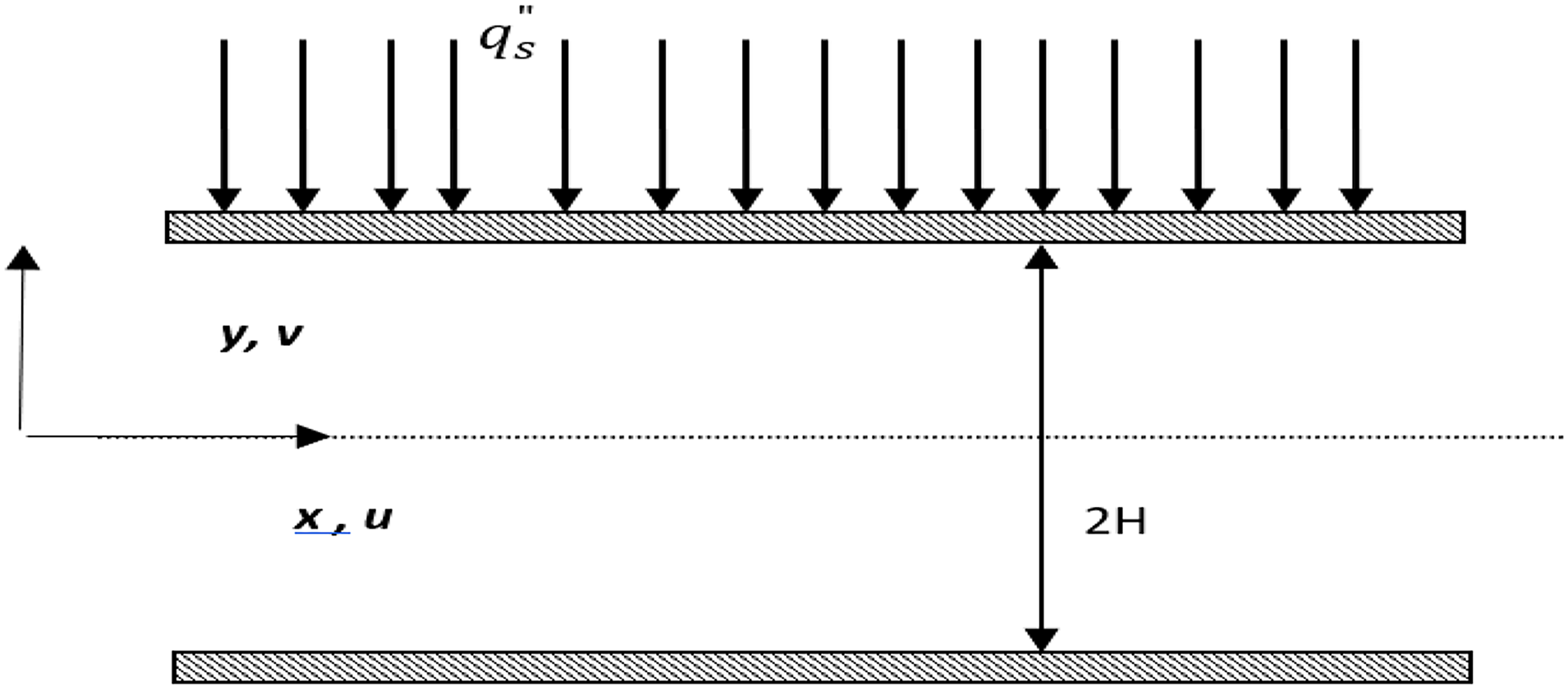
The spatial structure of the duct.
The methodology employed in this study offers several key advantages. By combining the Runge–Kutta fourth-order method for the coupled momentum equations with finite difference methods for the energy equation, the approach ensures high accuracy and stability in solving complex micropolar fluid flows. The dimensionless formulation allows generalization of results and systematic analysis of parameters such as microrotation, coupling constant, spin-gradient viscosity, Reynolds number, and Prandtl number. This comprehensive treatment enables precise prediction of velocity, microrotation, temperature distribution, and Nusselt numbers, providing detailed insights into the thermal energy storage performance of vacuum rectangular ducts.
The present study considers laminar, incompressible, and two-dimensional flow of a micropolar fluid within a vacuum rectangular duct. The fluid is assumed to exhibit microrotation effects and spin-gradient viscosity, while its physical properties, including density, viscosity, thermal conductivity, and specific heat, are considered constant. The duct walls are maintained under a constant surface heat flux, and no-slip and no-spin boundary conditions are applied. For the steady-state analysis, the flow is assumed fully developed, whereas entrance-region effects and daily solar irradiance variations are treated separately, allowing the examination of flow development and transient temperature profiles without altering the momentum equations. Body forces, buoyancy, and radiative effects are neglected, ensuring a focused and consistent analysis of the thermal energy storage performance of micropolar fluids. In the daily variation analysis, a quasi-steady approach is employed, where the steady-state equations are solved repeatedly using time-dependent surface heat flux values to simulate changing solar irradiance throughout the day. While this method does not capture true transient effects, such as fluid inertia or dynamic thermal response, it provides a practical and computationally efficient way to estimate temperature variations and thermal energy storage trends under realistic daily solar conditions. The results highlight periods of peak heat storage and allow evaluation of optimal micropolar fluid parameters for different times of the day.
Navier-Stokes equations can't model micropolar fluids, which have microstructures with molecules that can deform and rotate independently, the micropolar fluid model is a meaningful extension of the traditional Navier-Stokes model. It introduces an angular velocity field for particle rotation, and an additional vector equation for the conservation of angular momentum where the stress tensor lacks symmetry, the conservation law of angular momentum operates independently. This leads to the introduction of an extra equation, the micropolar fluid model includes the micro-rotation equation, enabling analytical solutions based on viscosity coefficients. It distinguishes between dynamic microrotation viscosity, measuring resistance to microrotation, and dynamic Newtonian viscosity, measuring shear resistance, resulting in two types of viscosity: linear and angular. Below, we propose the governing equations for the linear and angular movement and energy of the micropolar fluid in the described system, including the continuity equation for the fully developed region:
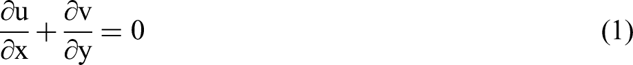
The continuity equation (Naterer, 2022):
The linear momentum equation (Naterer, 2022):

The angular momentum equation (Naterer, 2022):

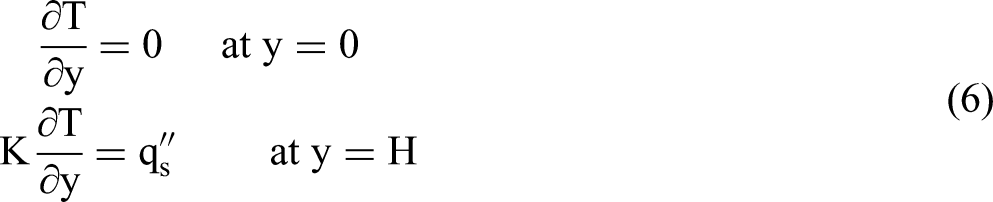
The energy equation (Naterer, 2022):

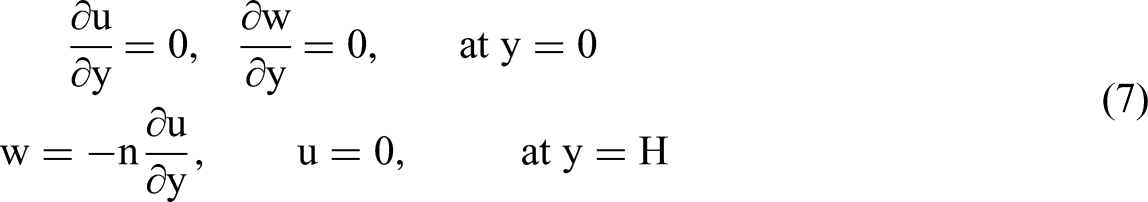
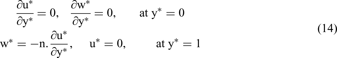
The following initial and boundary conditions (that are depended on both the hydrodynamic and thermal entrance lengths, considering that these two lengths are not equal in generally).
At

At
At
The effects of the micropolar fluid parameters are closely tied to the governing equations. For instance, the coupling parameter directly multiplies the microrotation terms in the momentum equations, influencing the velocity distribution and generating additional rotational stresses that alter energy transport. Similarly, the spin-gradient viscosity appears in the angular momentum equation, enhancing rotational diffusion and thereby increasing the local temperature through improved convective heat transfer. Reynolds and Prandtl numbers scale the convective and diffusive terms in the energy equation, governing the relative influence of advection and conduction. Scaling arguments show that higher coupling parameters increase fluid momentum but reduce thermal penetration depth, while higher spin-gradient viscosity enhances rotational energy dissipation and raises the mean temperature, explaining the trends observed in the numerical results.
The micro-gyration constant n ranges from 0 to 1, relating microrotation to shear stress. n=0 means no rotation; n=0.5 eliminates the asymmetric stress tensor; n=1 indicates turbulent flow. To simplify the governing equations for the micropolar fluid system, we make the following assumptions: steady-state, incompressible fluid with uniform properties in all directions, flow driven by an external force (e.g., a pump), laminar flow, negligible radiation effects, no thermal or mechanical energy generation, fully developed flow, constant surface heat flux, negligible viscous dissipation, and temperature below boiling point, The micropolar fluid pressure depends only on the
Hence, we have four differential partial equations to deal with. In the following we formulate these governing equations for fully developed regions with different set of boundary conditions, and with the following dimensionless variables definitions (Naterer, 2022):
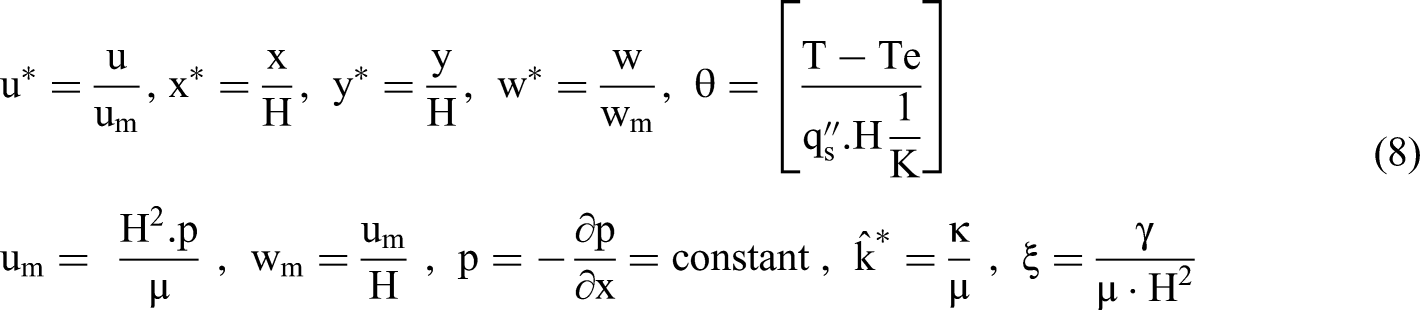
Where
Where
The important feature of hydrodynamic conditions in the fully developed region is that the radial velocity component


At
At
Numerical solution
For clarity and to demonstrate the realism of the nondimensional parameters, representative dimensional values are provided. The rectangular duct is assumed to have a height of 0.05 m and a width of 0.1 m. The micropolar fluid has a density of 1000 kg/m³, dynamic viscosity of 0.001 Pa·s, and thermal conductivity of 0.6 W/m·K. The surface heat flux is taken as 5000 W/m², consistent with typical solar thermal applications. Using these values, the dimensionless parameters—Reynolds number, Prandtl number, coupling parameter, and spin-gradient viscosity—fall within physically realistic ranges relevant to solar thermal energy storage scenarios.
This study employed numerical methods to solve the governing equations for steady state. The Runge-Kutta fourth order (RK4) method was used for coupled ordinary differential equations to find dimensionless velocity and microrotation, while the finite difference method determined dimensionless temperature based on boundary and initial conditions. All solutions were derived under constant surface heat flux conditions.
Runge Kutta Method (Solution of coupled linear & angular momentum):
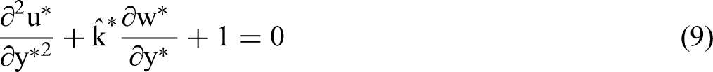
Solving the coupled non-dimensional equations of linear and angular momentum, represented in equations (9) and (10), using the Runge-Kutta method, specifically the fourth-order (RK4) method. This approach helps us determine the dimensionless transitional velocity (u*) and the dimensionless microrotation (w*) which are depend on y*.
The fourth-order Runge-Kutta (RK4) method is a popular numerical technique for solving ordinary differential equations (ODEs). It efficiently approximates solutions with high accuracy, making it a preferred choice for many applications., It uses four slope estimates (K) at each step to compute the next value, with a step interval of (h = 0.01).
Here are the steps detailing the use of this method:
Introducing a new variables to transform the higher-order system equation (second order) into a first-order equation, for equation (9) and (10).
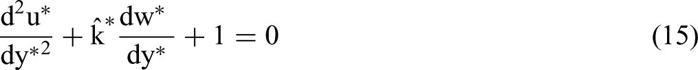


The system becomes: Once the equations have been rearranged and the new variables substituted, implement the Runge-Kutta method combined with the shooting technique. Define the system of equations as illustrated below: Establishing the boundary condition and providing the initial guess for the system


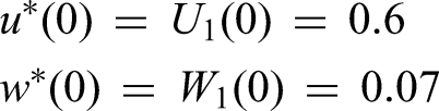
And the initial guess for the unknowns at y* = 0 are: Sixteen values of slopes (K) are calculated for each step, with four (4) values for each function, where the value of (K1) at the beginning of interval, (K2, K3) at the midpoint of interval, and (K4) at the end of interval. Next, calculate the values of U1, U2, W1, W2 after applying the following equation:


Continue iterating until the steps reach y* = 1 and compare the value with the boundary condition at this point if it is matching with it then the initial guess is correct otherwise adjust the initial guess value to achieve boundary condition.
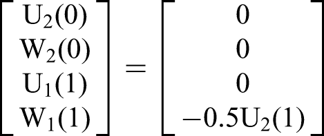
In MATLAB, this method utilized the built-in routine bvp4c, designed for solving boundary value problems. MATLAB requires converting these equations into a system of coupled nonlinear differential equations, represented in the matrix format below:
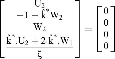
The boundary conditions required for the solutions are as follows:
Next, the system of equations is solved using MATLAB's bvp4c function. This function employs a three-stage Lobatto IIIa formula, ensuring accuracy and continuity within the specified interval. Finally, the outcomes are presented in the form of tables and graphs which illustrate in next section.
Numerical solution of constant surface heat flux in fully developed region for energy equation
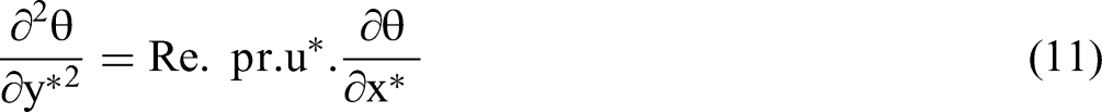
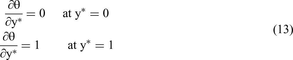
In this section shown the solving of the linear second order partial differential of the dimensionless energy equation (11), according to the initial and boundary conditions in the equations (13) by finite difference method using MATLAB. The partial differential equation was discretized to transform it into an algebraic for each node by approximation by Taylor expansion as shown below:


The finite difference approach to solve equation (3.20) is:

The finite difference method addresses the equation at specific, discrete points within the domain, known as grid points, as depicted in Figure 3. Here, Δy* indicates the step difference along the y-axis, while Δx* represents the step difference along the x-axis. The variables i and j correspond to the number of nodes along the x* and y* axes which were (100) for each, respectively, based on this number, Δx* and Δy* were set to (0.35, 0.01) respectively in order to obtain the solution of equation (11) in matrix form.
Assuming that Re and Pr are constant and u* is a function of y* after executive the Runge kutta code as shown previously, it was applied in the finite difference code. The discretized equation is used to form a linear system of algebraic equation in the following manner:

A matrix (N*N) was named (A) which is the N is the number of the nodes in the space and it was equal (104 * 104), and each row in this matrix represents the coefficient of (θ) for each node, while the matrix (b) shows the initial and boundary condition and its size was (104 * 1) and considering that the initial guess value of (θ) for all nodes on y* were equal (1), finally the system which aforementioned above equation (29) was solved by using inverse matrix:

The results of dimensionless temperature and dimensionless (mean and wall) temperature are presented in the form of graphs which illustrate in next section.
Numerical solution testing and results validation
To ensure the reliability of the numerical results, a comprehensive analysis of convergence, stability, and grid independence was conducted. The stability of the finite difference method (FDM) applied to the energy equation was assessed using the von Neumann stability criterion. As shown in Figure 2 (left), the numerical error decreases logarithmically as the time step size is refined, indicating a stable and convergent solution. Similarly, the convergence behavior of the Runge-Kutta fourth-order (RK4) method used for solving the momentum equations was analyzed. Figure 1 (right) demonstrates a consistent reduction in numerical error with decreasing step size, confirming the accuracy and stability of the RK4 method. Also, a grid independence study was performed by comparing numerical results at different grid resolutions (50 × 50, 100 × 100, and 200 × 200). Figure 3 presents the variation of the mean Nusselt number across these grid sizes. It was observed that the Nusselt number remains nearly constant between the medium (100 × 100) and fine (200 × 200) grids, with a relative difference of less than 1%. This confirms that the numerical solution is independent of further grid refinement, ensuring computational efficiency without compromising accuracy. Based on this analysis, the smaller grid was selected for the simulations, balancing precision and computational cost.
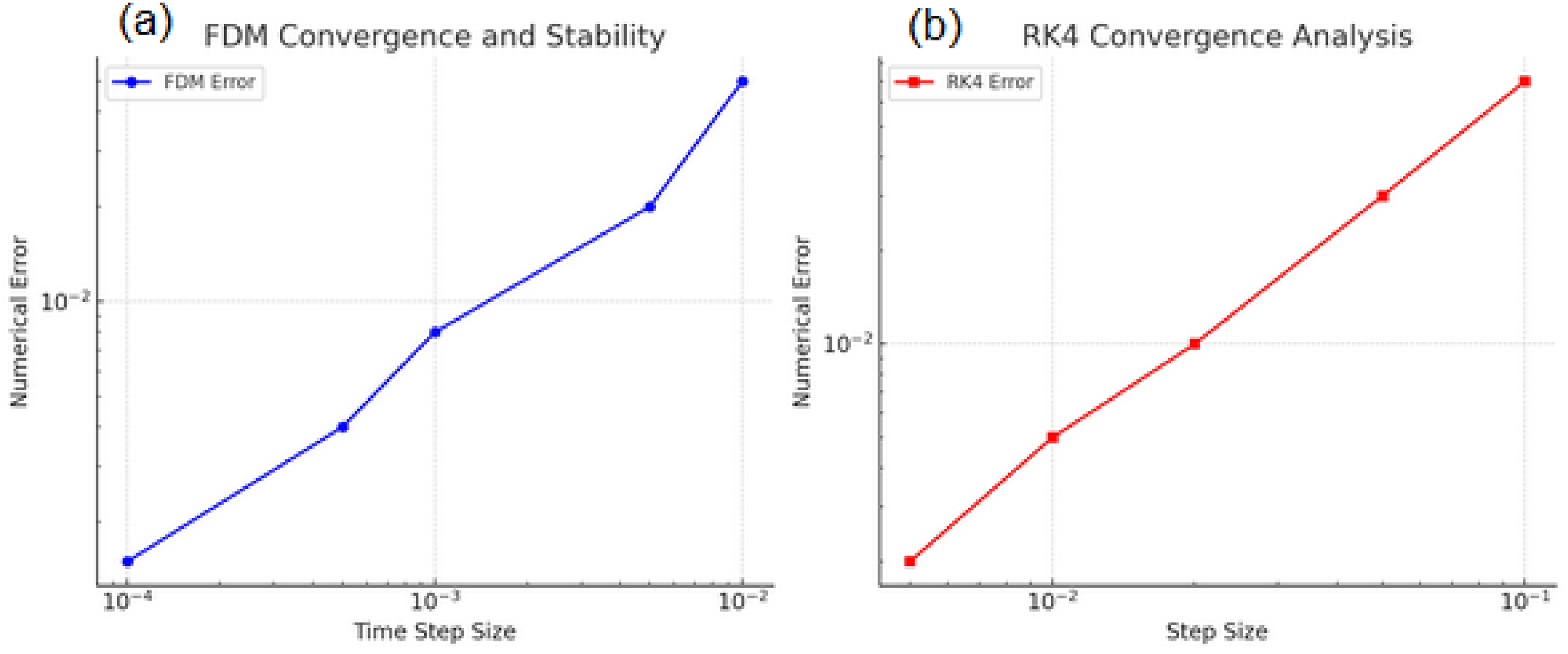
Convergence and stability of numerical solution for both FDM (a) and RK4 (b) methods.
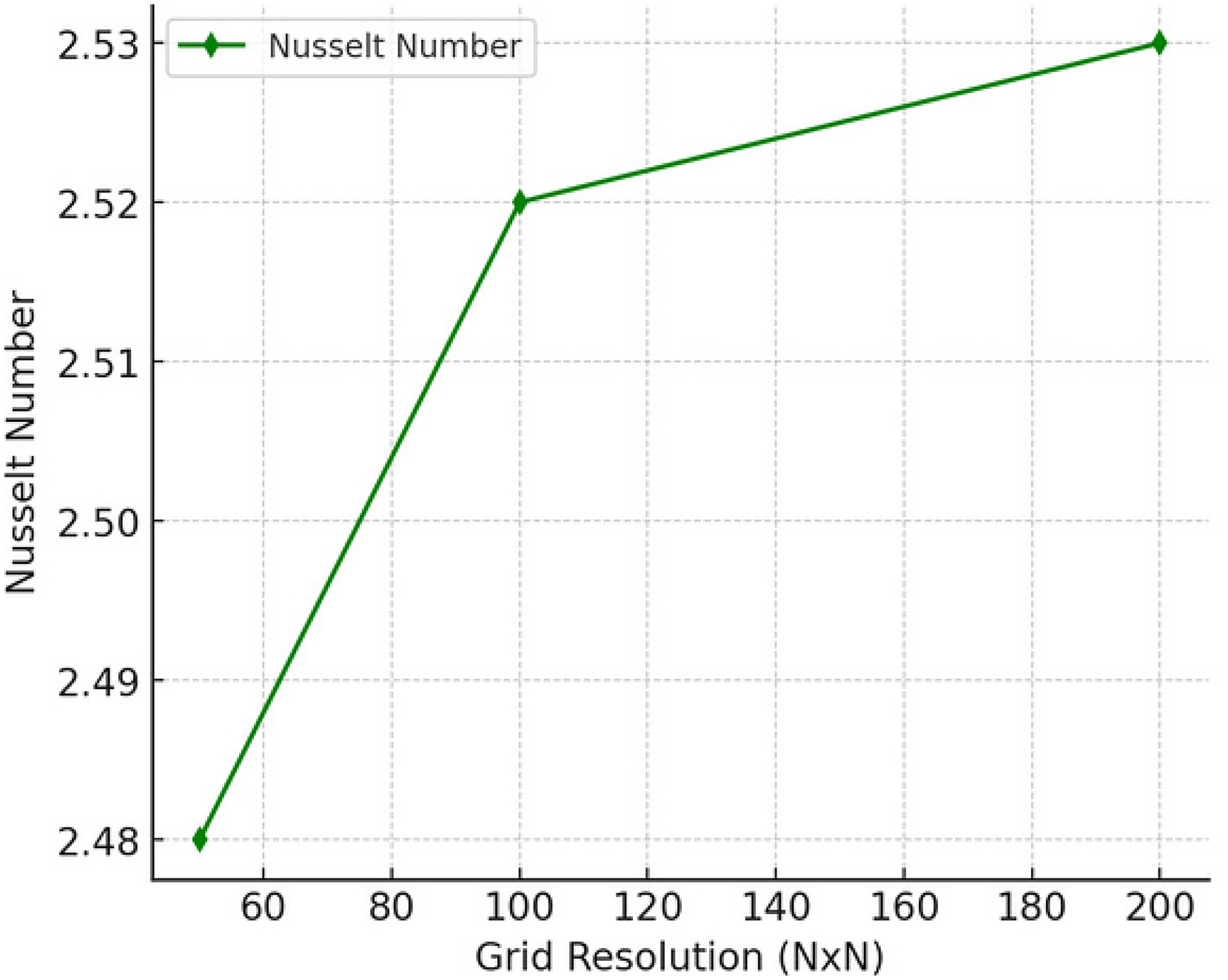
Grid independence study for the numerical solution.
The verification of the current codes for the numerical solution, using the Runge-Kutta fourth order (RK4) method and Finite Difference Method (FDM) were examined using previous research papers to ensure that the solution was correct. Considered the cases from the previous studies along with their boundary conditions and implemented them in the current codes used in this study. The papers dealt with two parallel permeable porous walls and a two-dimensional micropolar fluid flow between them (Jalili et al., 2023), and (Mirgolbabaee et al., 2017). Considering the following differences from the current study:
The previous studies utilized the stream function The dimensionless stream function and temperature varied only along the vertical coordinate. The applied boundary conditions were as follows:

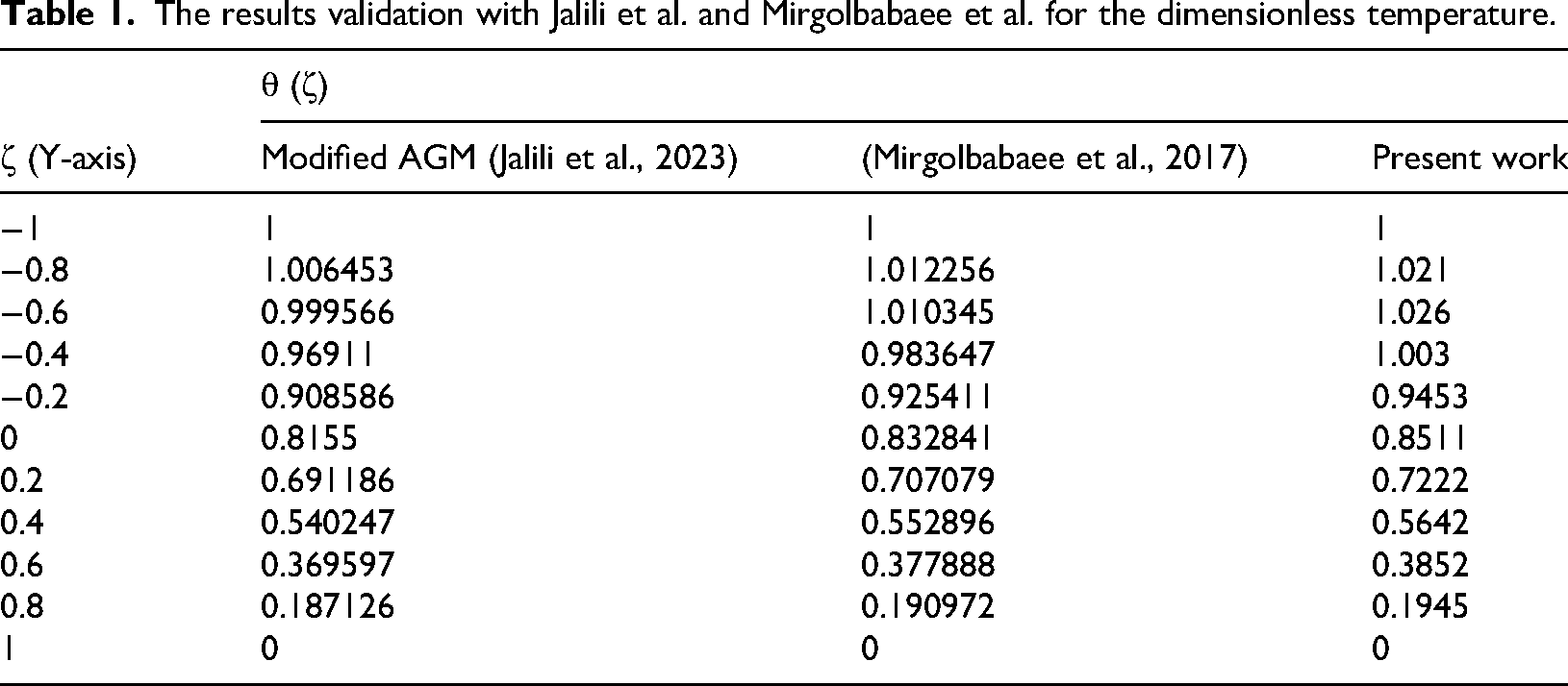
After implementing the RK4 and FDM numerical schemes to solve the linear and angular momentum, as well as energy equations, in MATLAB, the obtained results for the dimensionless stream function (f) and dimensionless temperature (θ) as a function of the y-coordinate were found to be in good agreement with those from the benchmark studies, as illustrated in Figure 4 and Table 1. This verification confirms the accuracy and reliability of the present numerical approach. The results demonstrate a high degree of convergence between the current and previous values for both dimensionless stream function and temperature, with an error rate not exceeding 0.86% indicated a strong agreement and compatibility between the previous and current results, validating the accuracy and reliability of the codes used in this study.
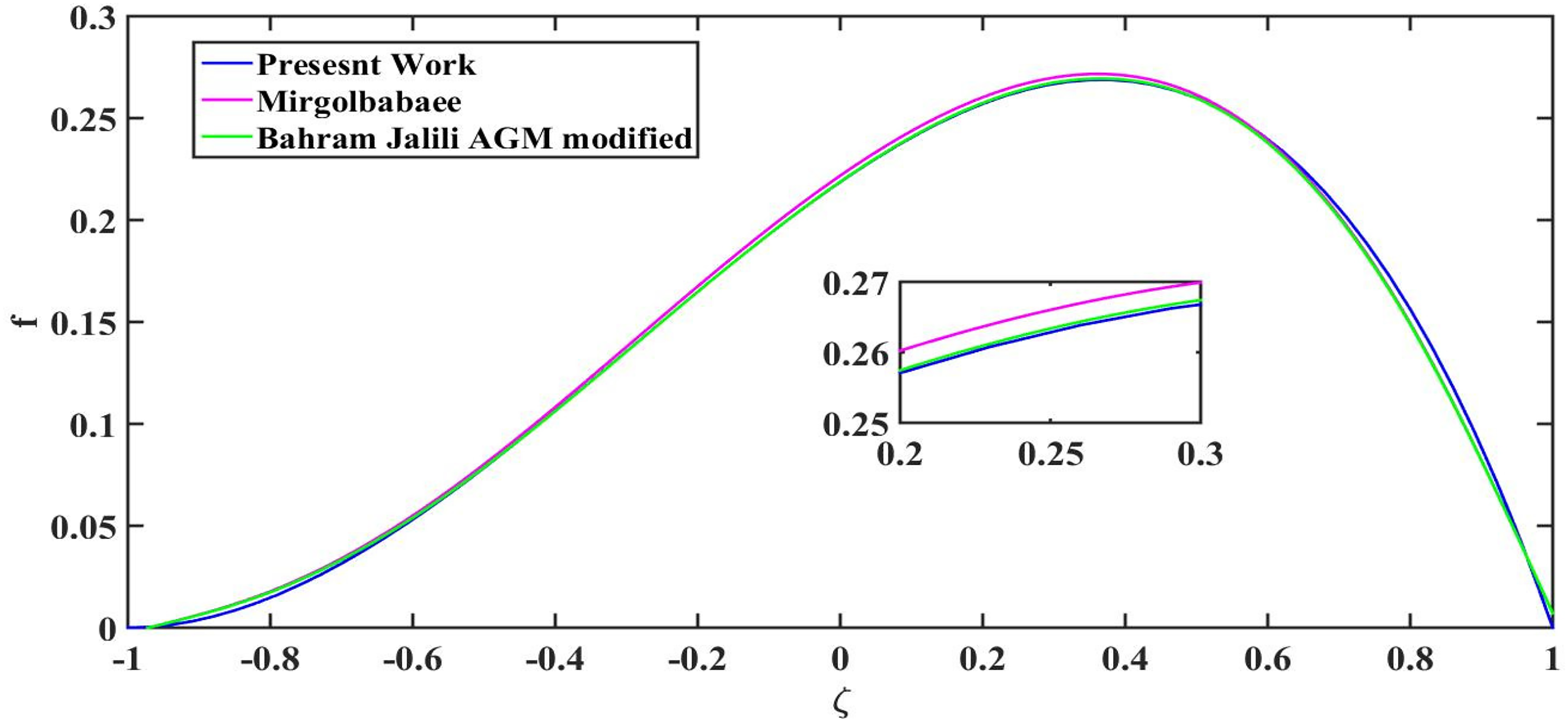
The results validation with Jalili et al. and Mirgolbabaee et al. for the dimensionless stream function f(y).
The results validation with Jalili et al. and Mirgolbabaee et al. for the dimensionless temperature.
Results and discussion
The findings of this study have important implications for practical thermal energy storage applications, particularly in solar energy systems and industrial heat exchangers. The ability of micropolar fluids to enhance heat transfer rates, especially in systems that require efficient thermal storage, could lead to improved performance in such applications. This research opens up possibilities for designing more efficient thermal energy storage systems using micropolar fluids.
The results were obtained for the fully developed region in the duct, with equations solved and presented in figures for transitional velocity, microrotation, Nusselt numbers (the ratio of convective to conductive heat transfer), and temperature profiles based on various parameters like coupling, spin gradient viscosity, Prandtl, and Reynolds numbers. Heat flux data were tailored for Amman using experimental data from the PVGIS website.
Dimensionless (transitional velocity and microrotation)
Figures 5(a) and 5(b) and Figures 6(a) and 6(b) illustrate the dimensionless translational velocity
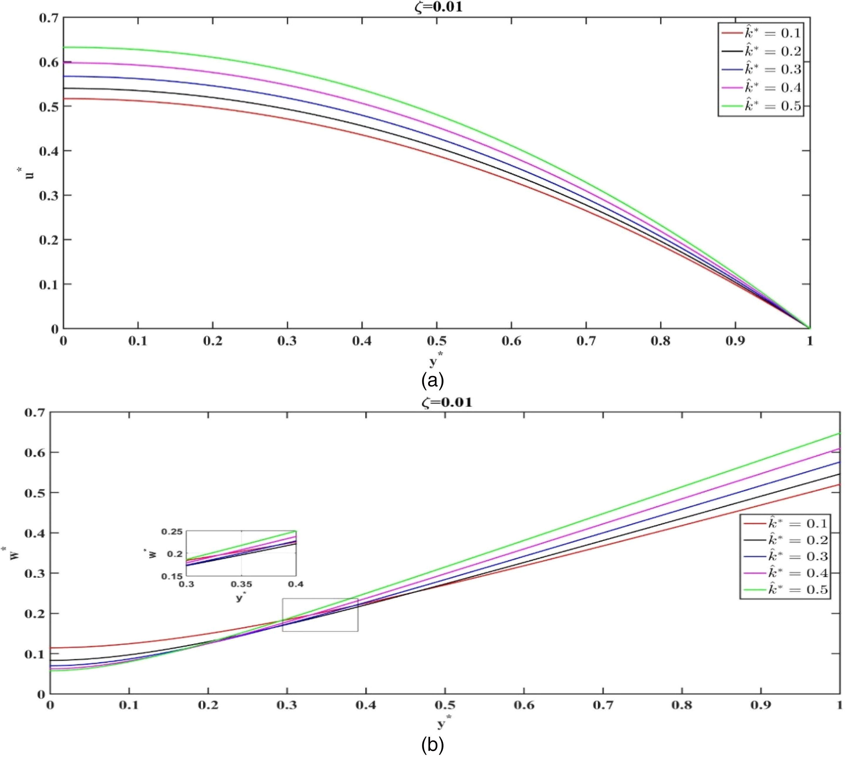
(a). Dimensionless transitional velocity with y* at different
Dimensionless temperature for different coupling parameters
Figure 7 (a) and 7 (b) illustrate the variation of dimensionless temperature
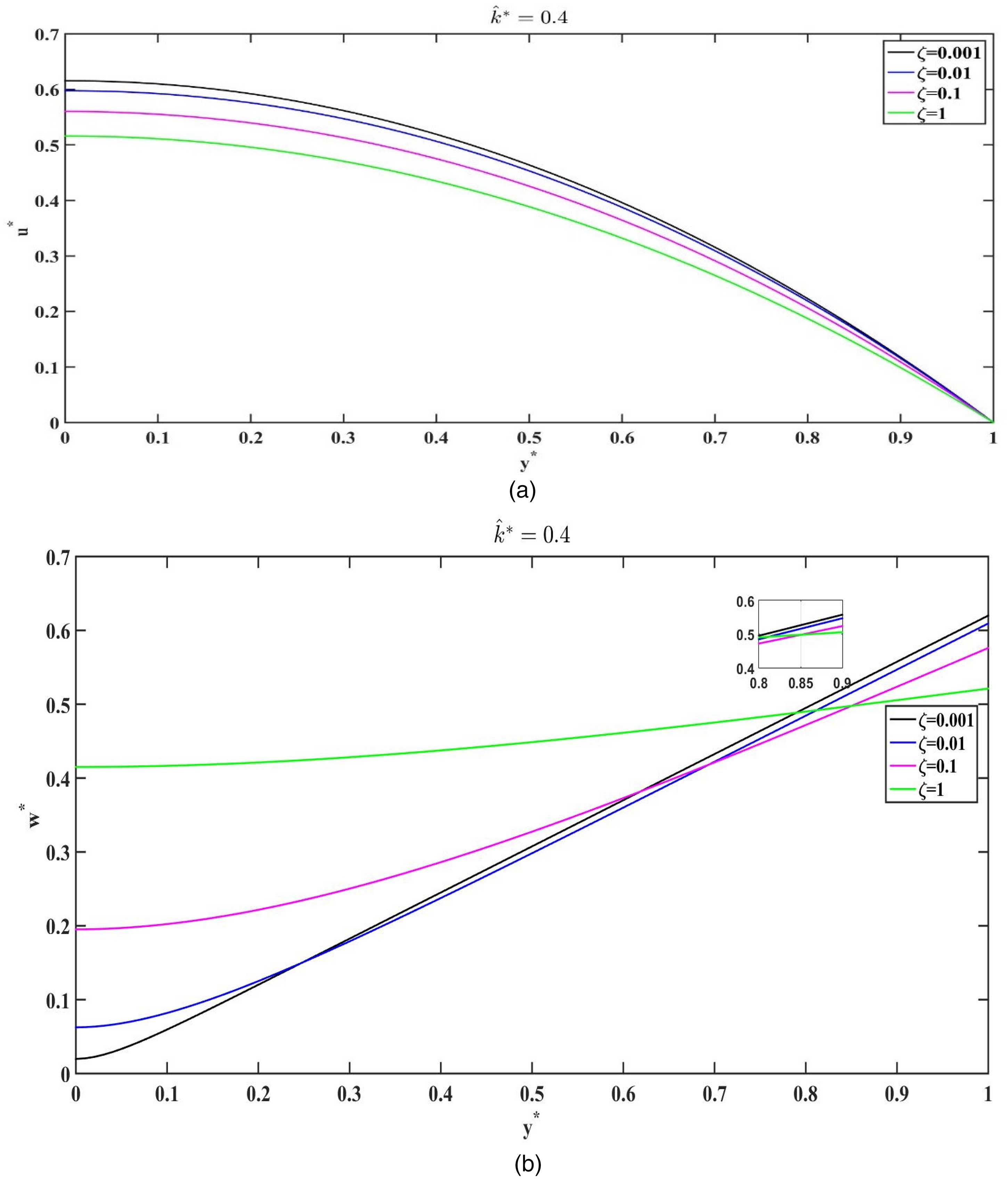
(a). Dimensionless transitional velocity with y* at different ζ. (b). Dimensionless microrotation with y* at different ζ.
Dimensionless temperature for different spin gradient viscosity parameters
Figures 8 (a) and 8(b) illustrate the effect of the spin-gradient viscosity parameter
Dimensionless temperature for different Reynolds number
The effect of Reynold number on dimensionless tempreture with y* for several points x* was represented in Figure 9 (a,b), the Reynold number is the ratio between inertia force and viscouss force so when increasing reynold number means that the viscouss force decreased so that the mean translational velocity will increase which may reduce the effectiveness capacity of energy stored in fluid layers.
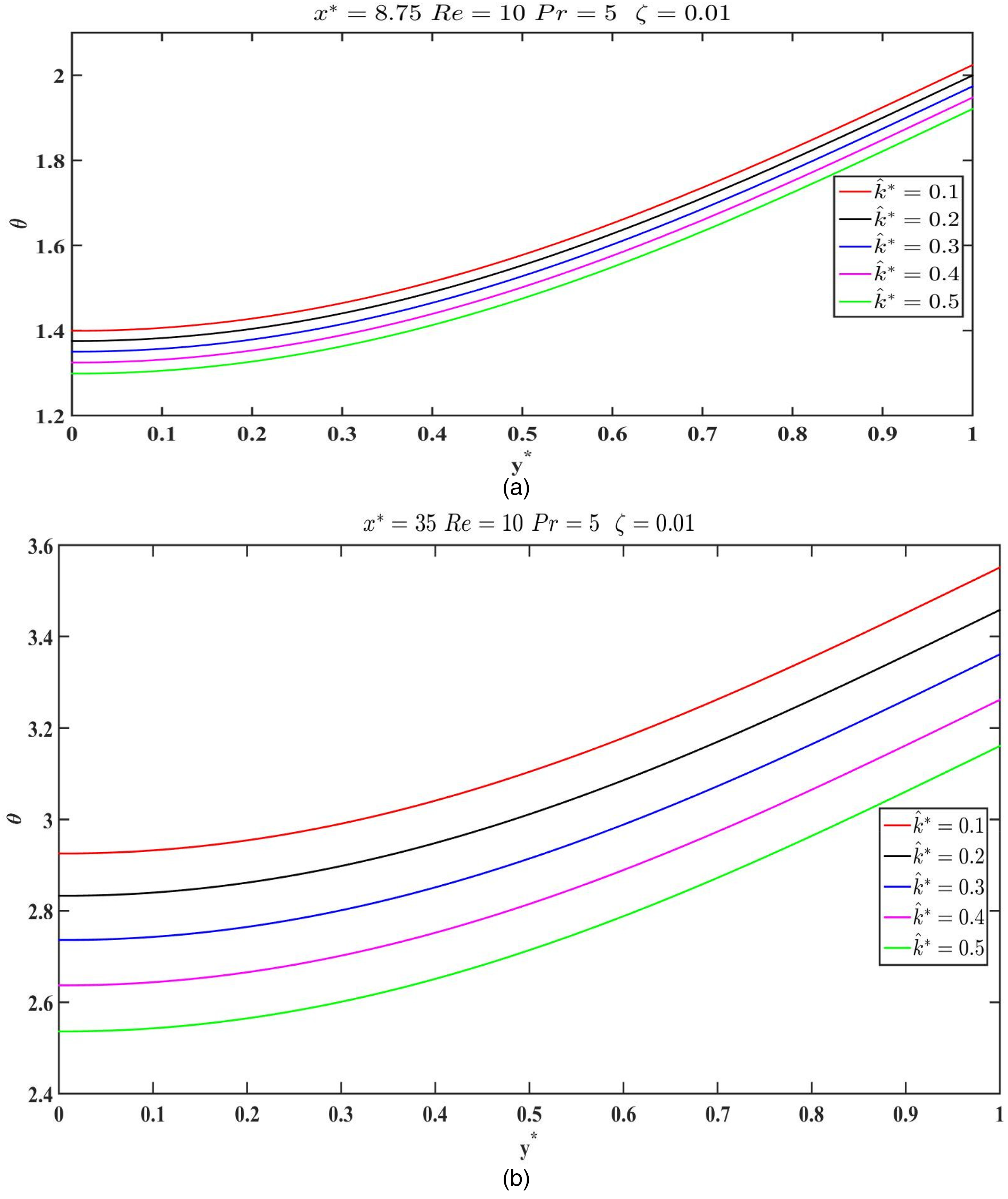
(a). Dimensionless temperature with y* at x* = 8.75 for different
Dimensionless temperature for different Prandtl number
Figures 10(a) and 10(b) depicts the effect of varying Prandtl numbers (Pr) on the dimensionless temperature
Dimensionless mean temperature
Figure 11 (a,b,c,d) depicted dimensionless mean temperature along the duct x* with selective values of coupling parameter, spring gradient viscosity parameter, Reynold number, and Prandtl number. It is clear from the previous figures when the Reynold number and Prandtl number rise up the dimensionless temperature decreased, because there are not enough time to capture more heat from solar source due to higher velocity and lower thermal conductivity respectively, thus the dimensionless mean temperature (average temperature) is going to be decreased on the other hand the impact of coupling parameter is inversely with mean temperature, but the spin gradient viscosity parameter is proportional with it, due to being coupled with velocity, and noticed that the dimensionless mean temperature increased linearly in case of constant surface heat flux.
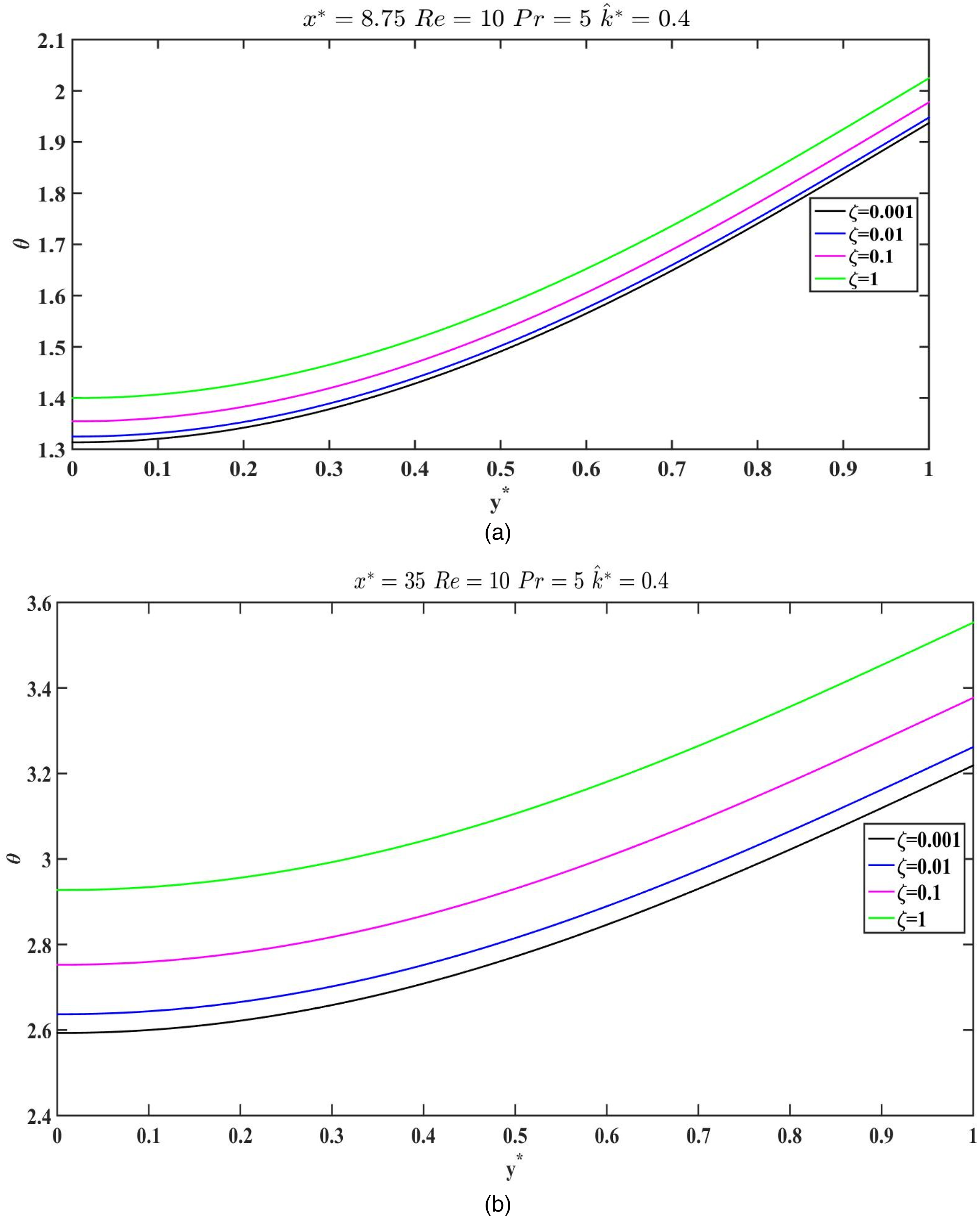
(a). Dimensionless temperature with y* at x* = 8.75 for different ζ. (b). Dimensionless temperature with y* at x* = 35 for different ζ.
Dimensionless wall temperature
Figures 12(a)-(d) illustrate the effect of the previously discussed parameters on the dimensionless wall temperature
Local Nusselt number
Figure 13 (a, (b), (c), (d)) discussed the local Nusselt number along the duct for selective values of parameters (
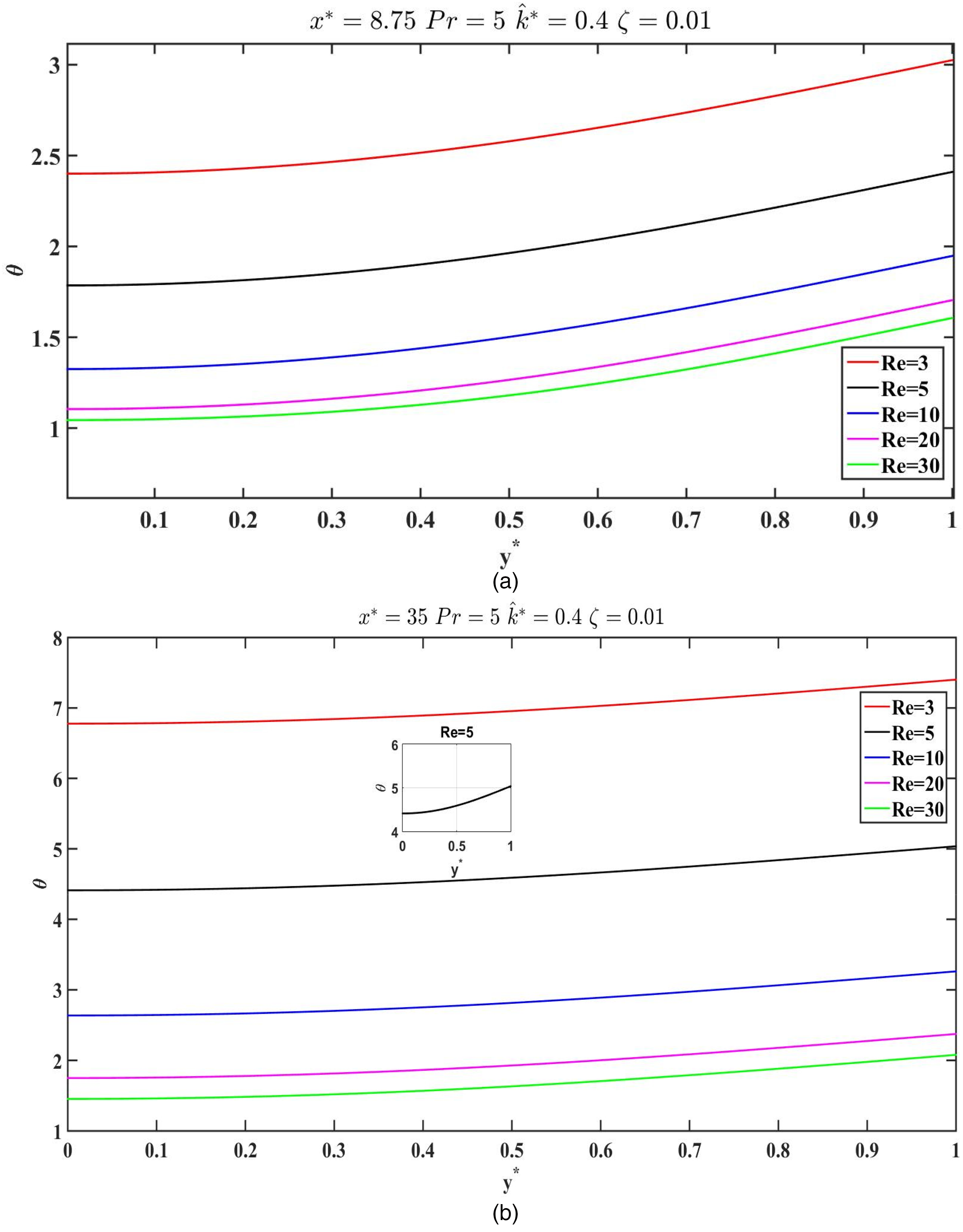
(a). Dimensionless temperature with y* at x* = 8.75 for different Re. (b). Dimensionless temperature with y* at x* = 35 for different Re.
Mean Nusselt number
Figures 14(a)-(d) presents the variation of the mean Nusselt number (
Temperature variation during the day at different heat flux
In Figure 15 (a), (b), (c), (d) as shown below represented the temperature difference between outlet and inlet mean temperature with hourly time for several values of heat flux in Amman for three months (January, June, and September), the data which was taken from PVGIS website according to equation 4.26. Two values of the variables (
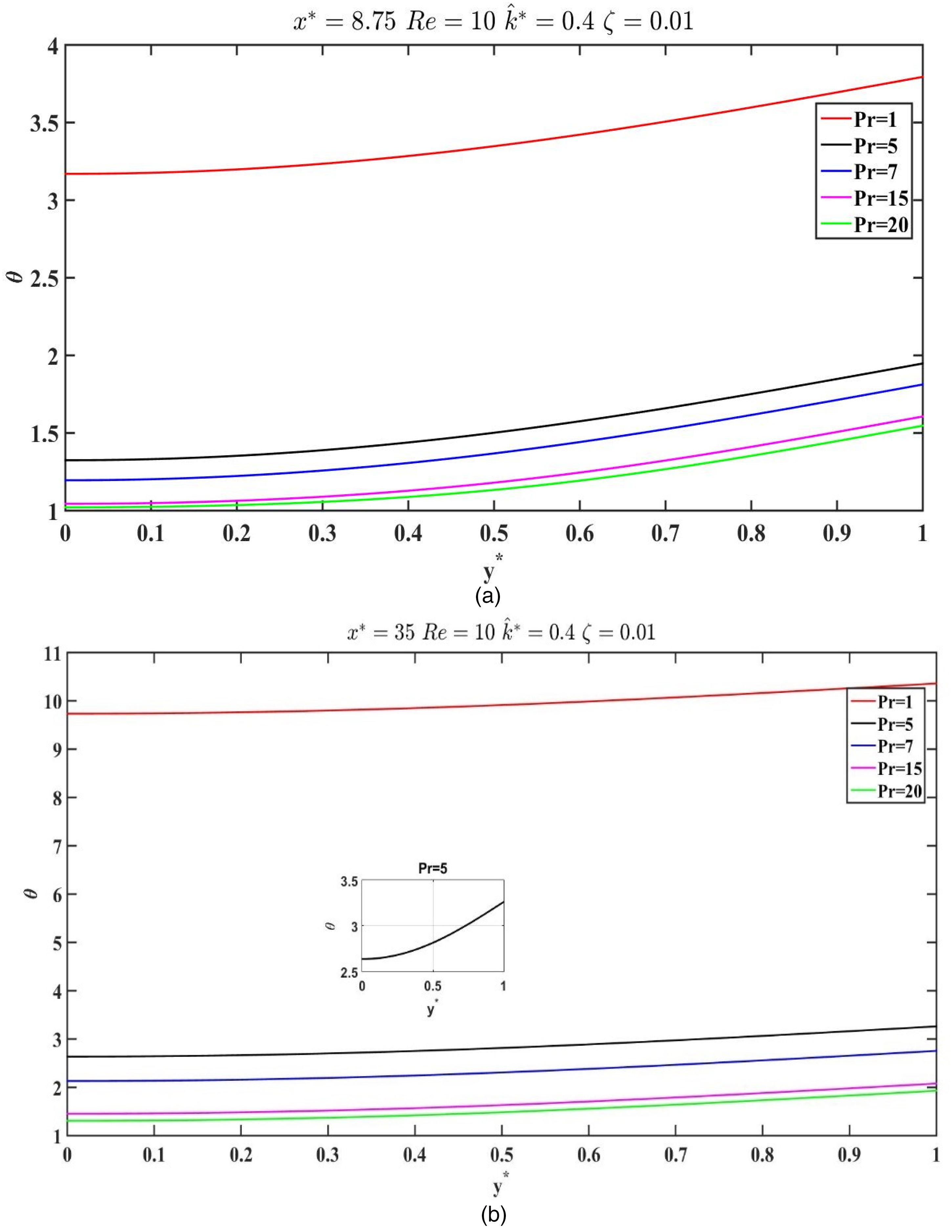
(a). Dimensionless temperature with y* at x* = 8.75 for different Pr. (b). Dimensionless temperature with y* at x* = 35 for different Pr.
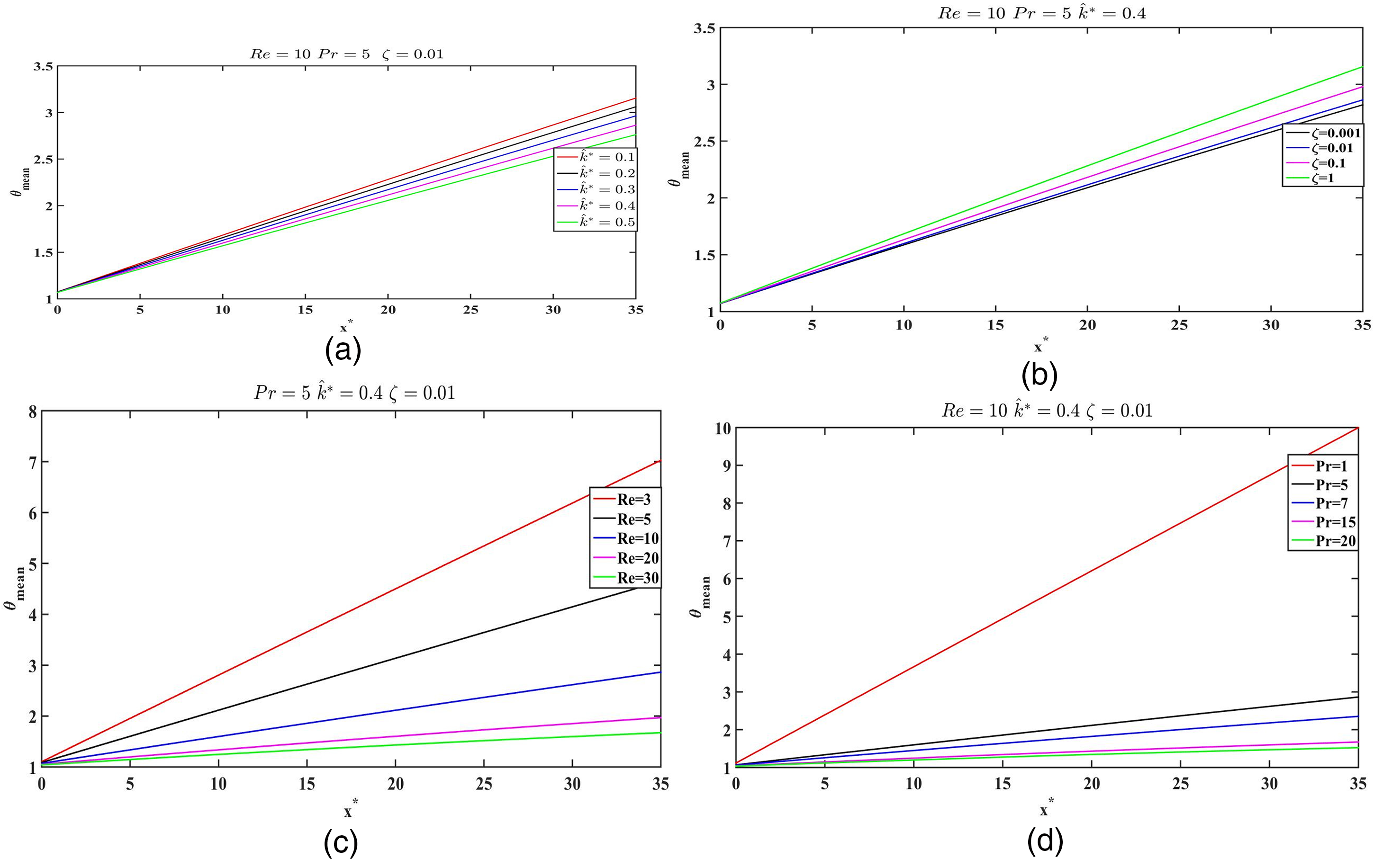
(a). Dimensionless mean temperature with x* for different
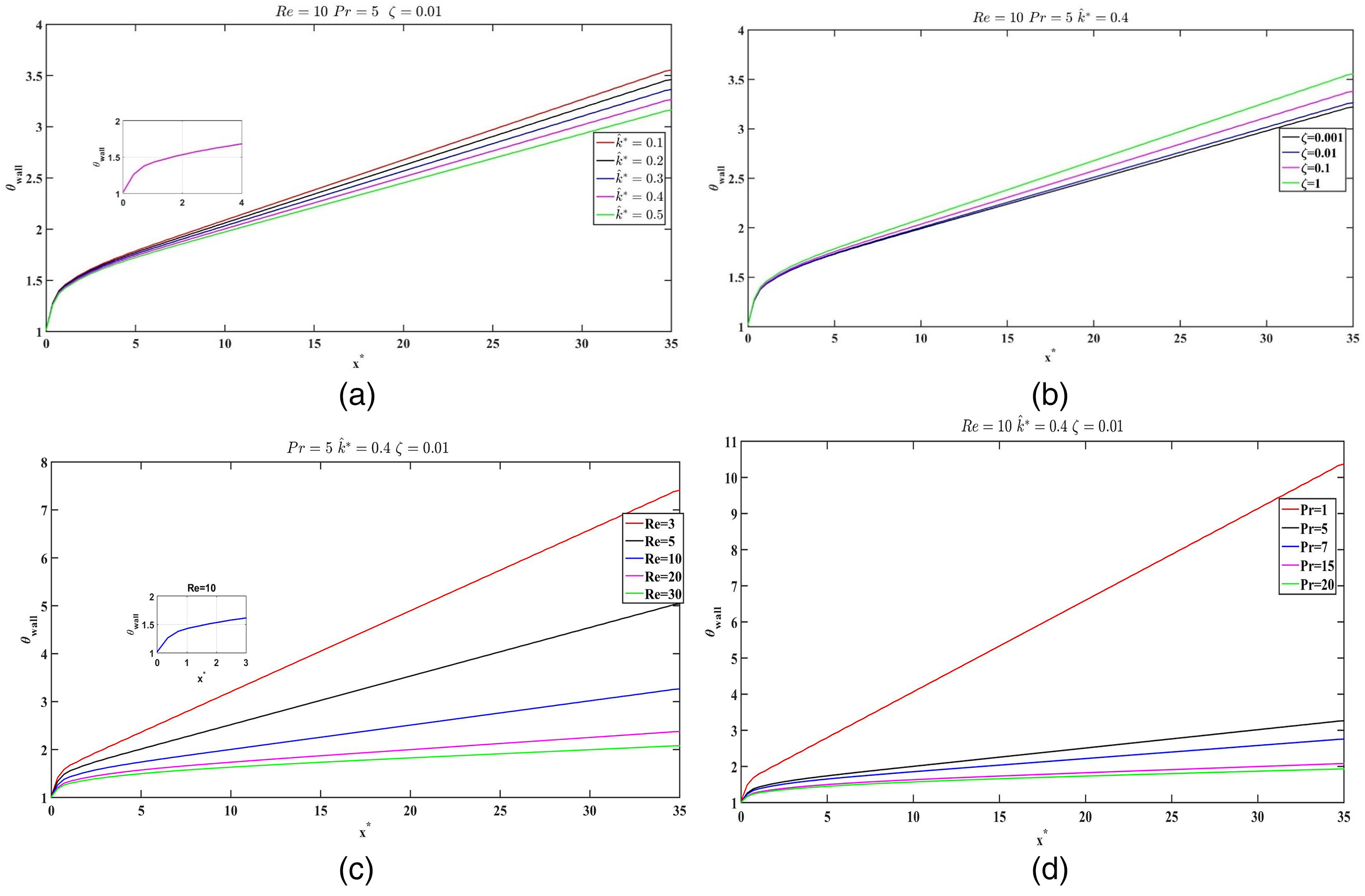
(a). Dimensionless wall temperature with x* for different
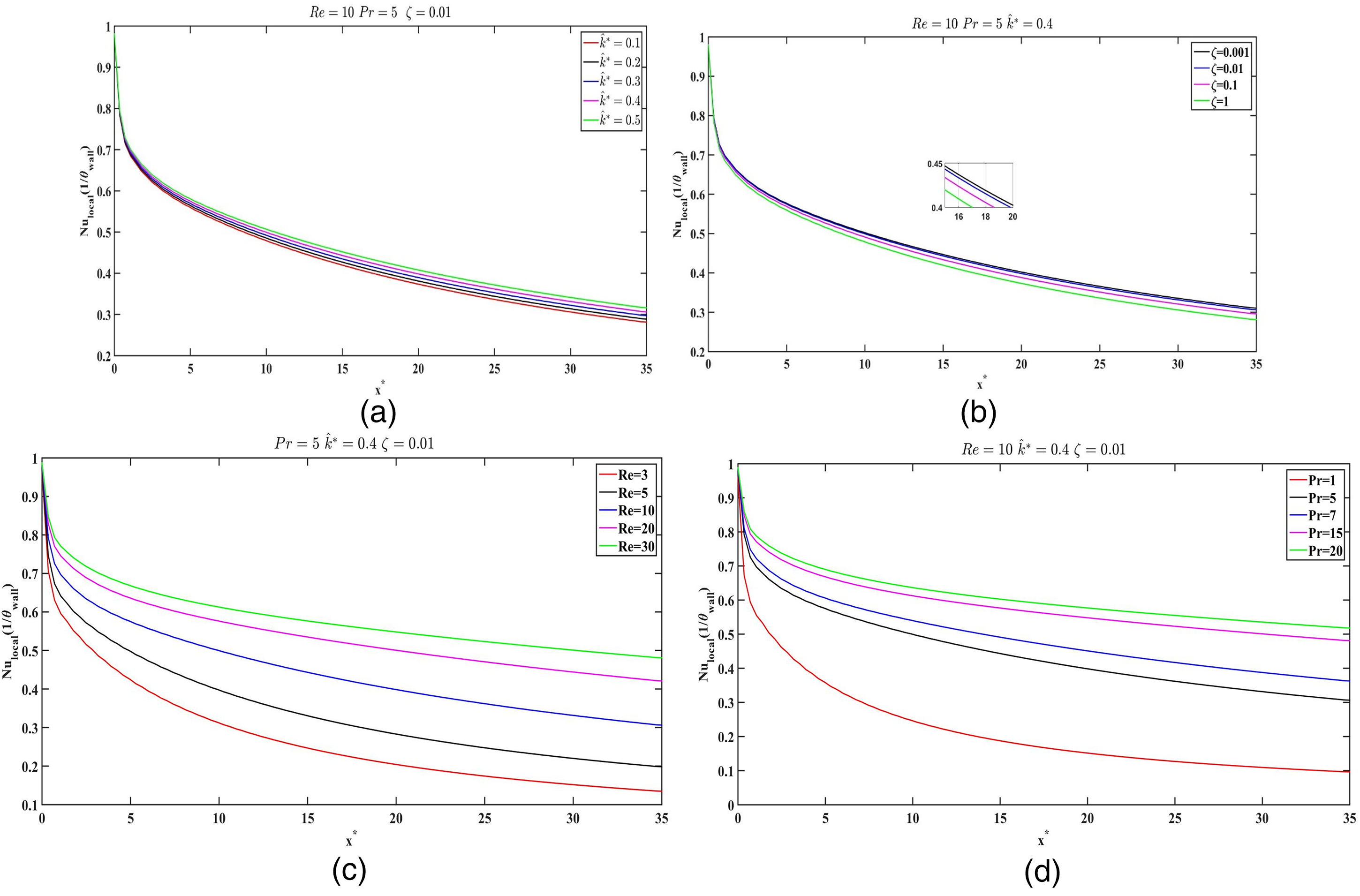
(a). Local Nusselt number with x* for different
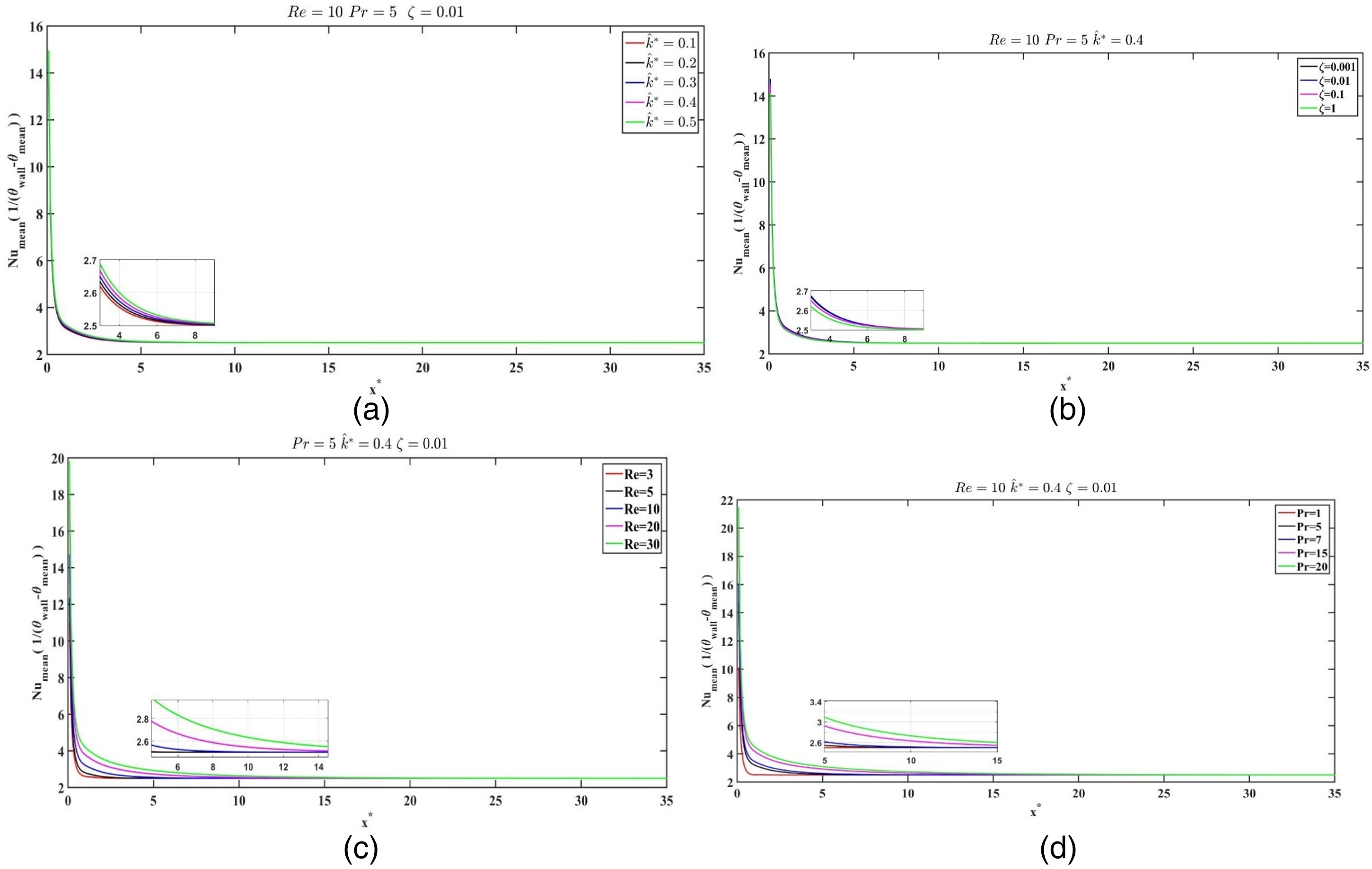
(a). Mean Nusselt number with x* for different
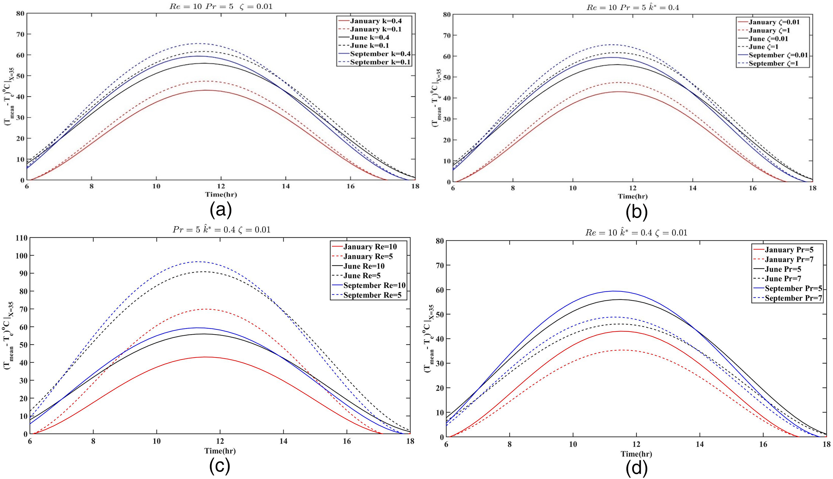
(a). Variation temperature with during the day for different heat flux and
Regarding the temperature variation during the day, the September temperature variation of 95°C was calculated using experimental data from the PVGIS website, which provides solar radiation and temperature data specific to the region. This data was used to estimate the temperature profile during a typical day in September, which was then used in the current model to simulate the temperature distribution and assess the heat transfer behavior.
Conclusions
This study presents a detailed numerical investigation of micropolar fluid flow and heat transfer in a steadystate vacuum rectangular duct, emphasizing their potential for thermal energy storage in solar applications. The results show that micropolar fluid parameters strongly influence flow and thermal behavior. Increasing the coupling parameter raised the dimensionless transitional velocity, while initially decreasing microrotation before it increased, leading to a reduction in the dimensionless temperature. In contrast, higher spring gradient viscosity enhanced temperature retention, improving the fluid's energy storage capacity. Reynolds and Prandtl numbers were also influential, with lower values supporting higher temperature variation and more effective heat storage.
Analysis of Nusselt numbers revealed that the mean Nusselt number stabilized around 2.53 at an entrance length of
Footnotes
List of Abbreviations and Symbols
Declaration of conflicting interests
The authors declared no potential conflicts of interest with respect to the research, authorship, and/or publication of this article.
Funding
The authors received no financial support for the research, authorship, and/or publication of this article.