Sage Journals: Discover world-class research

Abstract

Efficient energy management is crucial given 2024's 4.1% worldwide electricity demand increase. This urgency emphasizes the necessity for various, sustainable energy sources in distribution grids. Short-term load prediction approaches using probabilistic power generation and energy storage are crucial for energy usage prediction. Urban energy planners use simulation, probability optimization and modelling to create sustainable energy systems. This study offers a novel hybrid model for smart grids: short-term energy load prediction using transfer learning (TL) and optimized lightGBM (OLGBM). Our two-phase solution tackles Short-term Load Forecasting complexities. First, aberrant supplements and quick deviation selection eliminate missing values and identify key features during data pre-processing. Second, TL-OLGBM learns dynamic time scales and complex data patterns with Bayesian optimization of hyperparameters to improve forecasting accuracy. Additionally, our architecture easily combines the newest Smart and Green Technology, enabling energy system innovation. Comparative performance research shows that our technique outperforms similar models in mean absolute percentage error, accuracy and root mean square error. This hybrid model is a reliable short-term energy load forecast solution that fits the dynamic terrain of smart and green technology integration in modern energy systems.

Keywords

Energy transition resource utilization sustainability policies electricity load predication LightGBM

Introduction

Urbanization increased the requirement for power to power heating, cooling, lighting and other amenities. Population growth and the need for more residential and commercial space have driven up building energy use in recent years. Reducing building energy use helps meet decarbonization targets and lower energy costs for buildings, energy management and renters. As 2030 approaches and we accomplish carbon reduction goals, energy efficiency can be increased. Building owners and managers worry about energy performance since it affects their profits (Zhou et al., 2020). Making the energy management system intelligent and sustainable requires two-way information sharing between the utility and customers and long-operating equipment that can digitally react to quickly changing electric demand. Since commercial buildings like schools and businesses use so much energy, it is easy to understand how much money and energy we can save by making them efficient. The best way to boost building energy efficiency is ‘forecasting’. Historical data is used to forecast energy use and expenditures (Wan et al., 2021).

The expansion of building efficiency research and solution development has made building energy forecasting popular. Sensors and algorithms allow the grid to predict it. Buildings that purposefully use energy based on consumption and environmental considerations may be more profitable, efficient and sustainable. Energy consumption predictions can help facility managers and building automation systems identify energy use inconsistencies. Facility managers and building commissioning projects can save energy and optimize mechanical systems like chillers, boilers and energy storage units by predicting energy needs (Phyo and Jeenanunta, 2021). Forecasters predict client reactions to pricing changes, weather, global warming and personal finances hourly or weekly. Energy forecasters predict customer energy requirements to help utilities distribute resources. Innovative factors like energy management software and electric vehicle recharge concern them (Mamun et al., 2020).

The exponential growth of trustworthy ML datasets has made energy usage prediction and optimization a long-standing research area. Once a hotbed of academic research, load forecasting methods for predicting energy demands are now crucial to operations and power systems planning. Poor load forecasting affects power producing enterprises’ operational costs. Different groupings have formed based on how far ahead the projection is (Dokur et al., 2022).

Demand and utilities of energy

Energy is the ability to operate, whereas power is the speed. Energy is distance from A to B, while power is walking speed. However, building power is usually measured in W or kW. Most energy usage is classified by electricity use and heating/cooling needs. A building with electrical appliances needs power. A building's electricity use can be affected by ventilation, energy-efficient appliances, and conscientious occupants (Becirovic and Cosovic, 2016). To meet comfort standards, a tower's HVAC system must add or remove thermal energy from heating and cooling loads. Location, direction, season and interior design can alter a building's heating and cooling demands. Building management systems measure and report kilowatts or megawatts for external and internal loads (Jiang et al., 2018).

Energy demand and utility services cover several sectors and daily activities that consume energy differently. The breakdown of demand and utilities energy consumption is: In residential buildings, heating, cooling, lighting, cooking and running appliances use a lot of energy. Weather, family size and energy efficiency standards affect seasonal and regional energy demand in this industry. Commercial appliances, lights, HVAC and computers in schools, stores and offices need energy. Energy management technologies in business buildings boost efficiency and reduce costs. Industries use energy to power machines, heat materials and operate equipment. Energy-intensive industries including chemicals, cement and steel use energy efficiency methods to cut costs and boost competitiveness. Transportation, which uses fossil fuels for automobiles, trucks, buses, trains, ships and airplanes, uses a lot of energy. Alternative fuels and electric cars (EVs) are transforming transportation energy use, affecting power systems and charging stations. Utilities affect energy generation, transmission, distribution and supply. These individuals must manage power plants (coal, natural gas, nuclear or renewable), maintain transmission and distribution equipment, and provide energy-related services to consumers to meet changing energy demand. To improve reliability and sustainability, utilities invested in demand-side management, renewable energy integration and system enhancements. Due to renewable energy utilization, utilities are facing major energy demand shifts. Renewable energy technology can decarbonize the energy sector, reduce fossil fuel use and mitigate climate change. Thermal storage, pumped hydro and batteries are becoming more important for integrating renewable energy, improving grid resilience, and balancing supply and demand. Energy storage helps utilities manage peak demand, store renewable energy surplus and provide grid services like voltage support and frequency regulation. Distributed energy resources, advanced metering infrastructure, grid automation and demand response can assist utilities optimize energy distribution, stabilize systems and empower consumers to regulate their energy use. Smart grid deployments provide real-time monitoring, data analytics and predictive maintenance, improving grid responsiveness. Technology, legislation, the economy and consumer behaviours affect energy demand and utility services. We need a comprehensive approach that includes renewable energy deployment, grid modernization, energy efficiency and sustainable energy management to meet society's evolving energy needs.

Analysis of anticipated demand and supply

Without precise short- and long-term demand estimates, energy generation and transmission cannot be planned. These forecasts directly mirror real GDP growth. Electricity is essential for civilization's progress. Many nations have deregulated their electricity industry, making it a traded commodity in recent decades. The ‘Electric Power Act 54/1997 law’ in Spain left all parties apprehensive due to power costs and the inability to store large amounts of electricity. We present a simple framework for defining Spain's power usage and using index decomposition to analyze income elasticity in the short run. We'll also develop a precise load forecasting program to plan tomorrow's electricity use (Ouyang et al., 2019).

Predicting a structure's energy use is crucial to energy efficiency. Accurate predictions help manage chillers, boilers and energy storage devices, reducing energy use. They also allow energy consumption variations from forecasts to be recognized and addressed. A small amount of information is often available for such predictions. However, they must be precise (Deng et al., 2019). Analysts have studied power usage patterns using time series models and other statistical methodologies. We call ‘time series data’ a collection of measurements applied to the same variable throughout time. Recently, machine learning has been used to anticipate electricity consumption due to its ability to extract complex non-linear relationships (Kong et al., 2020). However, increases in computing capacity make deep learning approaches increasingly important for solving issues in numerous sectors. Deep learning models like LSTM networks handle time series (Xuan et al., 2021).

This research improves utility managers’ demand response decision-making by tackling energy load forecasting's difficulties. Our main contributions are as follows:

Innovative data-driven approach: We introduce a novel data-driven technique to predict moderate electricity usage. This approach employs a transformation-based hybrid model for energy prediction, incorporating the transfer learning method and optimize-LightGBM.

Two-phase methodology: The research unfolds in two distinct phases. Initially, we utilize an abnormal supplements strategy coupled with an immediate deviation selection technique to eliminate missing values and extract crucial features. Subsequently, we implemented the Transfer Learning-Optimize LightGBM (TL-OLGBM) approach with fine-tuned hyperparameters.

Transfer learning for dynamic patterns: The TL-OLGBM method proves instrumental in learning dynamic time scales and intricate data patterns. Bayesian optimization is employed for hyperparameter tuning, effectively addressing the challenges associated with Short-term Load Forecasting (STLF) and significantly improving forecasting accuracy.

Optimized LightGBM model: The final step involves the application of an optimized LightGBM model, seamlessly integrating both temporal and energy features to achieve precise energy forecasting.

Comparative performance analysis: Rigorous performance comparisons against existing methods demonstrate the superiority of our proposed model. The model outperforms standard empirical mode decomposition methods, showcasing considerably lower mean absolute percentage error (MAPE) and root mean square error (RMSE) values in simulation scenarios.

In summary, our contributions offer utility operators a robust and accurate tool for operational planning, navigating the intricacies of electricity load demand forecasting, and surpassing the performance of existing methods.

Related work

Here, we take a look at the best research done on the topic of using machine learning models to predict future power use. The use of machine learning in time series prediction is the subject of two recent reviews. To predict the price of energy one day in advance on the PJM market, Xuan et al. (2021) investigated an ANN model based on a similar days approach. The suggested model's superiority was demonstrated using publicly accessible data from the PJM Interconnection for training and testing the ANN. Constraints such as time, load and past prices concerning power price predictions are explored. The suggested ANN model based on the determination (2) of 0.6744 between load and power price is supported by simulation results. The similar day technique may reliably predict the PJM market's location marginal price.

Liu et al. (2017) designed the SVM model's free parameters, which was made possible by incorporating a diversity-guided model into the QPSO method, which we refer to as the AQPSO. Numerical investigations show that the model can increase accuracy, accelerate global convergence and shorten running times. The suggested model's efficacy is then demonstrated with instances using power load data from a Chinese city. The empirical findings support the claim that the proposed model is superior to the alternatives. As a result, the method is effective and feasible for predicting electric power system loads quickly. Marwala and Twala (2018) employed a genetic algorithm-trained support vector machine (GA-SVM) to predict future power prices. National power pricing data in China from 1996 to 2007 are utilized to examine it.

Microgrid short-term load forecast online learning model employing several classifier systems by Zhao et al. (2019). This model is built with many training sets fused using dynamic weighting. Experimental comparisons between the proposed technique and existing methodologies are made using data from a real-world Microgrid in Hong Kong. Chen et al. (Jawad et al., 2020) suggested a quick power market price forecast approach using the ELM. Using a bootstrapping process, the new method has increased confidence in its price interval forecasts. Using background data and examining daily routines, Gilanifar et al. (2020) identified several distinct daily behaviour patterns. We then gathered context features from various sources to develop a rule set that can be applied to any given day to predict the type of daily behaviour pattern with which it is most consistent. At the same time, a model was built to anticipate the load at a given time of day based on the volume of power used at that time and the type of behaviour pattern observed. This research focused on individual households in Taiwan as they sought a solution to the VSTLF. The suggested method outperformed the alternatives in terms of accuracy, achieving a MAPE of 3.23% for 30-min predictions of residential loads and 2.44% for aggregate loads.

Several machine learning techniques were tested (Naz et al., 2020), and their efficacy was measured against electrical load datasets. We examined the performance of SMOreg and additive regression methods for load forecasting using power consumption records. In addition, we analyzed STLF using ANN. The primary emphasis is to predict future electricity demand on a massive power infrastructure (Huang et al., 2020). Smart grid technology has advanced significantly in the past five years, becoming the industry standard for generating and distributing power. Dudek and Pełka (2021) provided a data-driven deep learning system to anticipate the short-term electricity load. First, the load data is processed using Box-Cox transformation.

Next, parametric Copula models are fitted to the data, and the peak load threshold is calculated. The proposed framework provides more accurate forecasts for the next day and the following week. A multi-scale convolutional neural network incorporating time cognition is the subject of a new proposal by Abdulrahman et al. (2021). The author successfully enhanced the sequential model of time cognition by designing a novel time coding approach termed periodic coding. Finally, a TCMS-CNN model that combines MS-CNN and irregular coding into a single framework for training and inference was presented.

For STLF, Azeem et al. (2021) described an integrated approach using EMD, comparable day techniques and DNNs. Notably, our suggested method considers the power price a significant determinant for load variance. There are two primary levels: feature extraction and forecasting layers. The load time series is decomposed using EMD in the feature extraction layer. The components are organized into a two-dimensional input matrix for CNN. The LSTM layer receives both the CNN output vectors and the raw load sequences. Therefore, the multimodal spatial–temporal characteristics are extracted from the input data using the whole EMD-based CNN-LSTM technique.

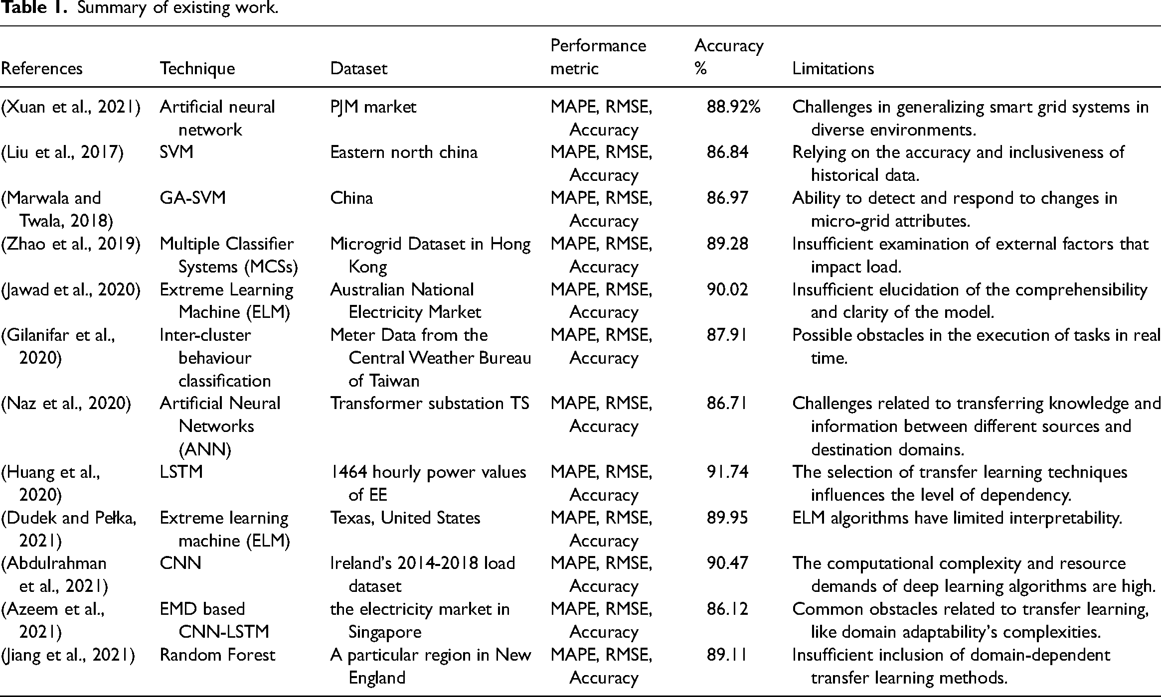
Several strategies, including analysis techniques, statistical tools, and computational intelligence, have been suggested to predict statistics on energy usage. To help decide which input features should go into the load forecasting model, Jiang et al. (2021) presented a random forest-based feature selection technique. A multi-model fusion STLF approach is proposed. The input features have been picked (CNN-BiGRU). Multiple CNN-BiGRU models are trained independently utilizing input data gathered via lengthy sliding time windows of varying steps. The final forecasted load value is the mean of the forecasts from several models. Table 1 shows the summary of existing work.

Table 1.

Summary of existing work.

References	Technique	Dataset	Performance metric	Accuracy %	Limitations
(Xuan et al., 2021)	Artificial neural network	PJM market	MAPE, RMSE, Accuracy	88.92%	Challenges in generalizing smart grid systems in diverse environments.
(Liu et al., 2017)	SVM	Eastern north china	MAPE, RMSE, Accuracy	86.84	Relying on the accuracy and inclusiveness of historical data.
(Marwala and Twala, 2018)	GA-SVM	China	MAPE, RMSE, Accuracy	86.97	Ability to detect and respond to changes in micro-grid attributes.
(Zhao et al., 2019)	Multiple Classifier Systems (MCSs)	Microgrid Dataset in Hong Kong	MAPE, RMSE, Accuracy	89.28	Insufficient examination of external factors that impact load.
(Jawad et al., 2020)	Extreme Learning Machine (ELM)	Australian National Electricity Market	MAPE, RMSE, Accuracy	90.02	Insufficient elucidation of the comprehensibility and clarity of the model.
(Gilanifar et al., 2020)	Inter-cluster behaviour classification	Meter Data from the Central Weather Bureau of Taiwan	MAPE, RMSE, Accuracy	87.91	Possible obstacles in the execution of tasks in real time.
(Naz et al., 2020)	Artificial Neural Networks (ANN)	Transformer substation TS	MAPE, RMSE, Accuracy	86.71	Challenges related to transferring knowledge and information between different sources and destination domains.
(Huang et al., 2020)	LSTM	1464 hourly power values of EE	MAPE, RMSE, Accuracy	91.74	The selection of transfer learning techniques influences the level of dependency.
(Dudek and Pełka, 2021)	Extreme learning machine (ELM)	Texas, United States	MAPE, RMSE, Accuracy	89.95	ELM algorithms have limited interpretability.
(Abdulrahman et al., 2021)	CNN	Ireland's 2014-2018 load dataset	MAPE, RMSE, Accuracy	90.47	The computational complexity and resource demands of deep learning algorithms are high.
(Azeem et al., 2021)	EMD based CNN-LSTM	the electricity market in Singapore	MAPE, RMSE, Accuracy	86.12	Common obstacles related to transfer learning, like domain adaptability's complexities.
(Jiang et al., 2021)	Random Forest	A particular region in New England	MAPE, RMSE, Accuracy	89.11	Insufficient inclusion of domain-dependent transfer learning methods.

Material and methods

This section covers the working of the proposed model and dataset description.

Dataset

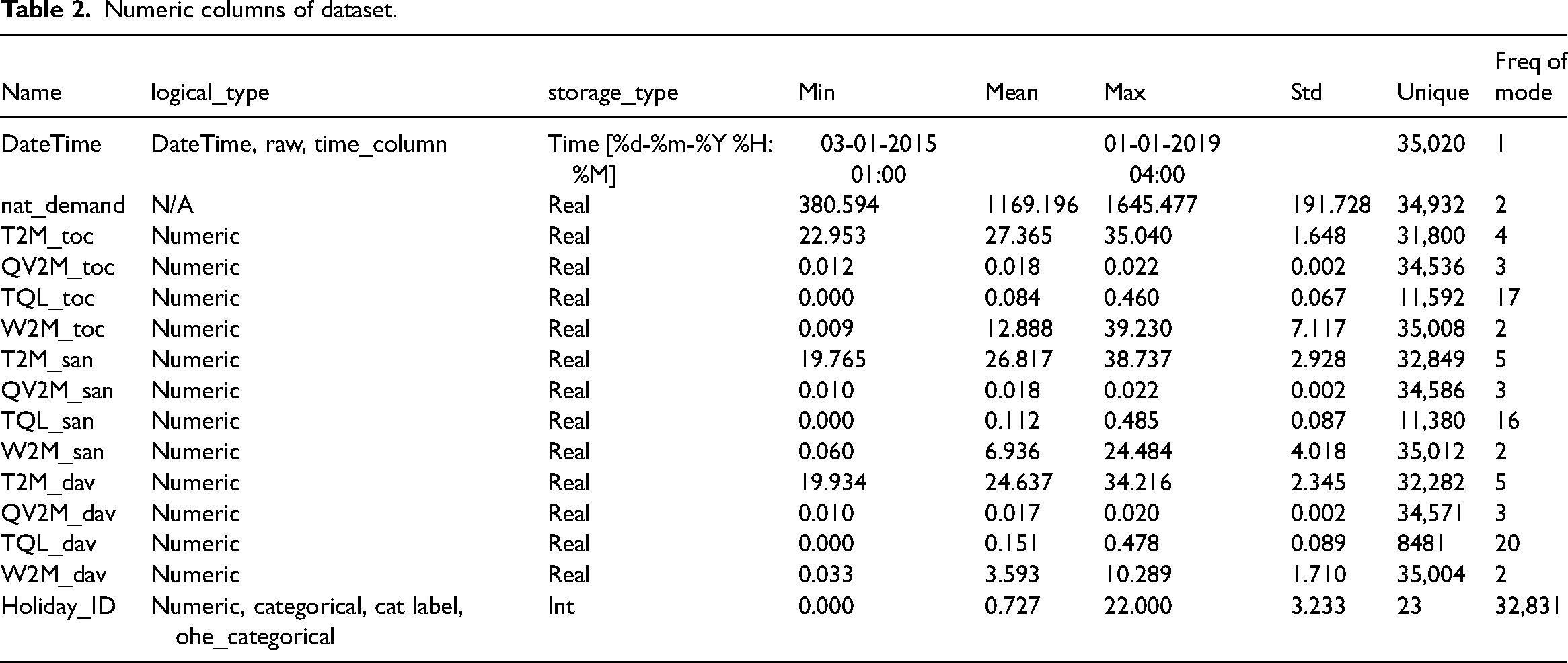
The dataset was collected from ‘The University of California (UCI) Machine Learning Repository’, named ‘Electrical Grid Stability Simulated Dataset’ (Dataset, 2023). The training data taken has only numeric columns and is shown in Table 2.

Table 2.

Numeric columns of dataset.

Name	logical_type	storage_type	Min	Mean	Max	Std	Unique	Freq of mode
DateTime	DateTime, raw, time_column	Time [%d-%m-%Y %H:%M]	03-01-2015 01:00		01-01-2019 04:00		35,020	1
nat_demand	N/A	Real	380.594	1169.196	1645.477	191.728	34,932	2
T2M_toc	Numeric	Real	22.953	27.365	35.040	1.648	31,800	4
QV2M_toc	Numeric	Real	0.012	0.018	0.022	0.002	34,536	3
TQL_toc	Numeric	Real	0.000	0.084	0.460	0.067	11,592	17
W2M_toc	Numeric	Real	0.009	12.888	39.230	7.117	35,008	2
T2M_san	Numeric	Real	19.765	26.817	38.737	2.928	32,849	5
QV2M_san	Numeric	Real	0.010	0.018	0.022	0.002	34,586	3
TQL_san	Numeric	Real	0.000	0.112	0.485	0.087	11,380	16
W2M_san	Numeric	Real	0.060	6.936	24.484	4.018	35,012	2
T2M_dav	Numeric	Real	19.934	24.637	34.216	2.345	32,282	5
QV2M_dav	Numeric	Real	0.010	0.017	0.020	0.002	34,571	3
TQL_dav	Numeric	Real	0.000	0.151	0.478	0.089	8481	20
W2M_dav	Numeric	Real	0.033	3.593	10.289	1.710	35,004	2
Holiday_ID	Numeric, categorical, cat label, ohe_categorical	Int	0.000	0.727	22.000	3.233	23	32,831

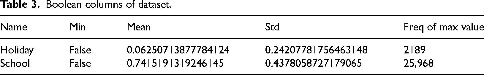
In our study, data preprocessing plays a critical role in ensuring the quality and relevance of the input data for our predictive model. The main steps involved in our data preprocessing phase are as follows: First, the authors fix any incorrect or missing numbers in the dataset. This is an essential step since it guarantees that our model will be trained on trustworthy data. Depending on the type of missing data, the authors use methods like imputation or elimination of missing values. The authors employ feature selection to decrease dimensionality and enhance model efficiency. This entails weeding out superfluous or unimportant features and picking out the most important ones that help with the prediction. The methods that the authors use include ranking features’ importance, conducting correlation analyses and selecting based on domain knowledge. The authors normalize or standardize all input features to make sure they are all roughly the same size. This phase guarantees that the model can converge effectively during training and prevents some features from dominating the learning process because of their bigger magnitude. Because smart grid energy demand data is inherently time-sensitive, the authors group it into appropriate intervals (such as hourly or daily) in order to more accurately detect trends and patterns. Data noise and unpredictability can be reduced through aggregation, yet crucial temporal information can be retained. The authors use methods like one-hot encoding or label encoding to convert any categorical variables in the dataset to a numerical representation. This makes sure that machine learning algorithms that take numbers as input will work. Dataset outliers have the potential to degrade the prediction model's accuracy. In order to avoid training a model with erroneous data, the authors use outlier detection algorithms to find and eliminate them. Table 3 shows Boolean columns of datasets.

Table 3.

Boolean columns of dataset.

Name	Min	Mean	Std	Freq of max value
Holiday	False	0.06250713877784124	0.24207781756463148	2189
School	False	0.7415191319246145	0.4378058727179065	25,968

Shapley values

A practical method with solid theoretical backing, Shapley's explanations provide coherent and consistent global and local feature contributions. The prediction of a regression model is the total of the contributions of local Shapley features and the bias term. They add the forecast to the link function in classification tasks (Chen et al., 2021). Figure 1 shows the Shapley summary, generated by randomly selecting 10,000 rows (the random selection for this plot is controlled by the auto-doc max rows option). Approximating the original features with these explanations depends on the frequency with which the components are employed in converted features and the importance of those transformed features to the final model. Each altered feature receives the same weight as the original features that went into making it. Each unique characteristic is then tallied according to this metric (Jiang et al., 2021).

Figure 1.

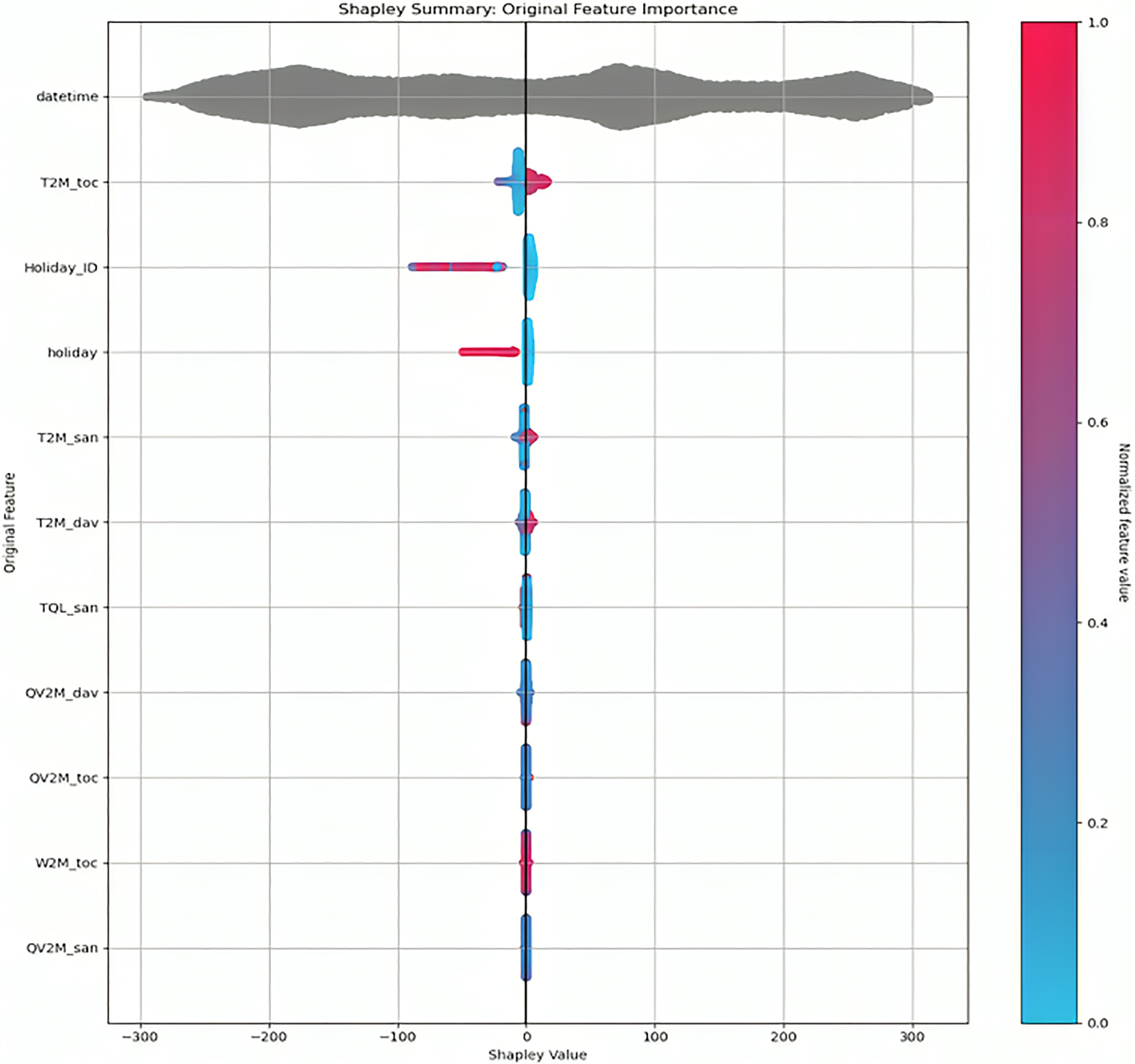
Shapley's importance.

Gradient boosted machines

Due mainly to the superior performance of decision trees relative to other machine learning methods, Gradient-boosted machines and their versions supplied by numerous communities have garnered much popularity in recent years. For example, XBoost and LightGBM are two of the most widely used algorithms for Gradient boosted machines (Obst et al., 2021). LightGBM eliminates data-heavy overhead. Collectively, they form the basis of the model's success and provide an advantage over competing for GBDT frameworks.

Architecture

It is a gradient-boosting framework that uses tree-based learning methods and is regarded as a very efficient computational approach. This algorithm has a reputation for being extremely efficient (Han et al., 2021). LightGBM process develops vertically, expanding leaf by leaf, whereas other algorithms extend horizontally, like a tree. Light-dependent gram-negative bacteria choose the leaf with the most loss on which to thrive (De Vilmarest and Goude, 2022). The schematic of leaf-by-leaf tree development in Figure 2 illustrates this.

Figure 2.

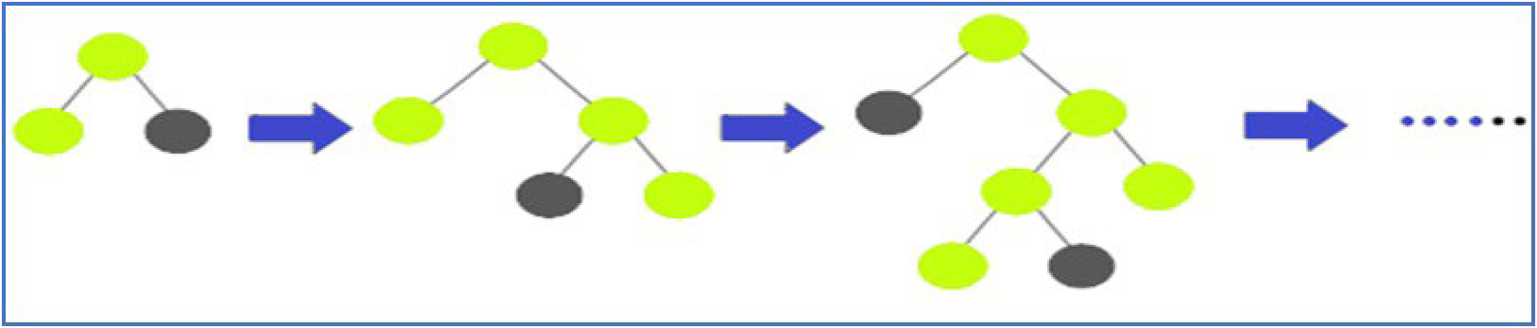
Leaf-wise tree growth.

Figure 2 shows how LightGBM, a key part of our suggested hybrid model for smart grid short-term energy load prediction, uses a leaf-wise tree growth technique. The more conventional depth-wise growth approach is at odds with this strategy. By dividing the tree at the leaf that improves the objective function (delta loss) the most, the algorithm builds the tree in a leaf-wise fashion. For quicker convergence and better utilization of computational resources, this approach gives priority to nodes that result in the largest loss reduction. Also, unlike depth-wise growth, it usually results in trees that are deeper yet have fewer leaf nodes. As data sizes grow exponentially, existing algorithms cannot provide timely results. LightGBM gets its name from its increased computational efficiency and speed of result delivery. It functions with reduced RAM use and can process massive volumes of data. More than a hundred LightGBM settings are included in the LightGBM documentation, but you don’t have to learn about them all. First, let’s look at some of the settings (Mousa et al., 2022; Ziel, 2022). To split the characteristics (Ci) for an independent point Pi, a Gain function (GF) can be defined in equations (1)–(3) as:

G F (P i) A = \frac{1}{C} (G F 1 (P i) + G F 2 (P i)

(1)

Where:

G F 1 (P i) = \frac{1}{C l} (G F 1_{a i ε A l} g k + \frac{1 - a}{b} \sum_{a i ε A l} g k)^{2}

(2)

G F 2 (P i) = \frac{1}{C h} (G F 2_{a i ε A h} g k + \frac{1 - a}{b} \sum_{a i ε A h} g k)^{2}

(3)

Proposed hybrid model

This research proposed a hybrid short-term energy load prediction model based on transfer learning with LightGBM for smart grids. The complete process utilizes three phases. Figure 3 shows the proposed hybrid model for the short-term energy load prediction model.

Figure 3.

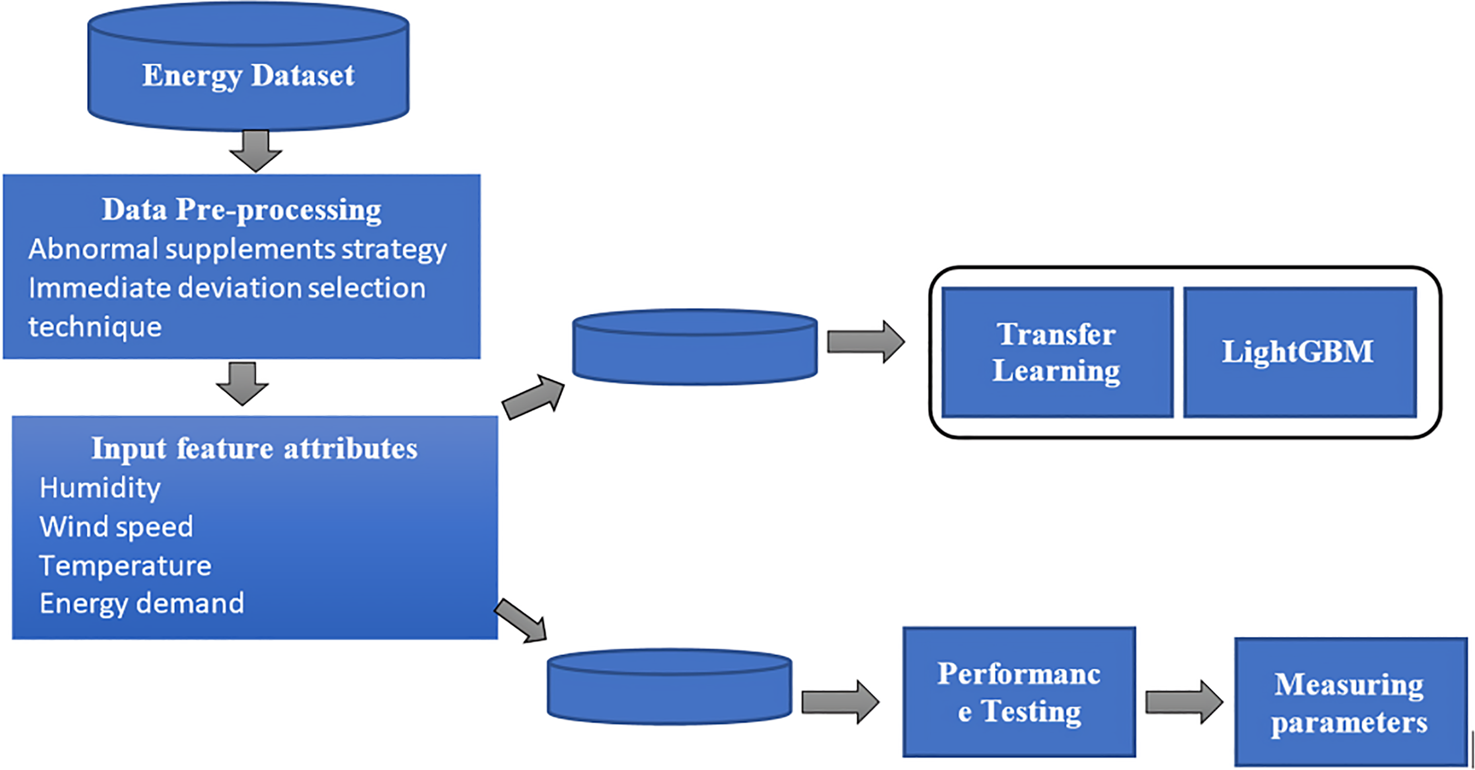
A proposed hybrid model for the short-term energy load prediction model.

The proposed model first applies data pre-processing using an abnormal supplements strategy with an immediate deviation selection technique. This phase eliminates the missing values and extracts the required features. The second phase uses a TL-OLGBM with hyperparameters. The TL method helps to learn the dynamic time scale and complex data patterns and the hyperparameters tuned via the Bayesian optimization technique, which addresses the challenge of STLF and increases forecasting accuracy. Finally, an optimized LightGBM model is applied, combining the time and energy features to predict effective energy forecasting.

Control parameters

The following control parameters were used.

Max depth: It specifies the maximum allowed model overfitting and tree depth. Lower the maximum depth if you suspect overfitting is occurring in your model (Chung et al., 2022).

Min data in leaf: The minimal amount of records required by the leaf is called the min data in the leaf and is used to prevent the model from overfitting.

Feature fraction: Every time a tree is built, a new random parameter is selected by feature fraction. If it's 0.7, it indicates we’d be using 70% of the parameter.

Bagging fraction: Bagging fraction ensures that only a specified fraction of the data is utilized in each cycle. This method is commonly employed to quicken training cycles while preventing overfitting.

Early stopping round: The process will cease if the validation data metric has not improved throughout the previous early stopping round iterations. Less careless iterations will result.

Lambda: It explicitly describes regularization. There is a continuous scale from 0 to 1 for its values.

Foundational factors

Following control, foundation factors were used.

Task: Describe the action to be taken on the data. Data may be used for either training or prediction.

Application: Whether or not to do regression or classification is set by the ‘Application’ option. The regression application parameter is selected by default in LightGBM.

Binary: A binary system helps make categorization decisions.

Multiclass: To solve issues involving many classes, or ‘multiclass’, it is applied.

Regression: Its most common use is regression analysis.

Boosting: This identifies the specific algorithm being used.

Rf: Random Forest, abbreviated rf.

Goss: One-Sided Sampling with Gradients.

Num_boost_round: Number of boosting rounds (Num boost round).

Learning_rate: The learning rate is used to determine how much of an adjustment is made to the approximation based on the output of each tree. It can take on 0.1, 0.001 and 0.003.

Num leaves: It provides the total number of leaves in a complete tree; its default value is 31.

Dimensional metric

It prevents loss even when the model is being constructed. Examples of some of these are shown below for both classification and regression.

Mae: Measuring the average of all mistakes made.

Mse: Error quantified by its square root; abbreviated Mse.

Binary_logloss: ‘Binary Classification Loss’ or ‘Binary log loss’ for short.

Multi_logloss: Multi Classification Loss (Multi log loss)

Modifying the settings

Tuning parameters is a common task for data scientists looking to improve accuracy and results in speed and handle overfitting (McHugh et al., 2022). To achieve optimal performance, we can try adjusting the listed parameters.

num_leaves: To begin, the model's difficulty may be traced back to the num leaves option. The optimal range for its values is below or equal to 2.

Min_data_in_leaf: Under fitting, the model might occur if a considerable value is given to the Min data in the leaf parameter. For massive datasets, several 100 or 1000 will do.

Max_depth: The third parameter, max depth, controls how deep the tree may go.

Several settings, or hyperparameters, are available in the LightGBM algorithm (Hadjout et al., 2022). Figure 4 shows the basic functioning of LightGBM.

Figure 4.

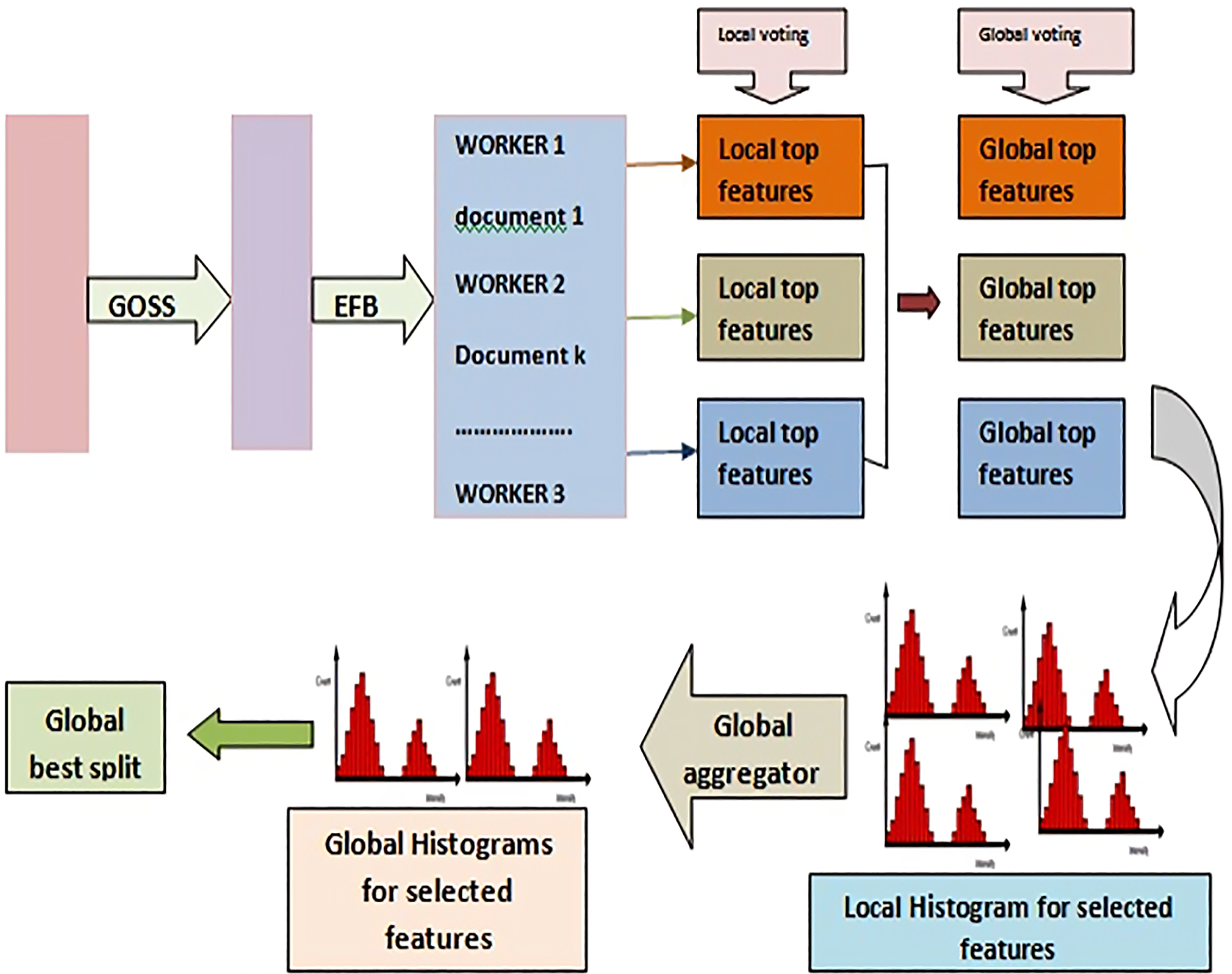
Schematic illustration of optimized LightGBM model.

The effectiveness of the LightGBM algorithm is very sensitive to the values chosen for its hyperparameters. Most of the time, they need to be manually adjusted and fine-tuned. The hyperparameters of the LightGBM algorithm are tuned with the help of a Bayesian-based hyperparameter optimization algorithm that is cleverly included in the suggested technique in this study. The maximum depth of the tree (‘max depth’), the number of leaves (‘num leaves’), and the learning rate (‘learning rate’) are examples of hyperparameters that may be fine-tuned. LightGBM is the proposed method's foundation since it can group otherwise disjoint features into a single bundle.

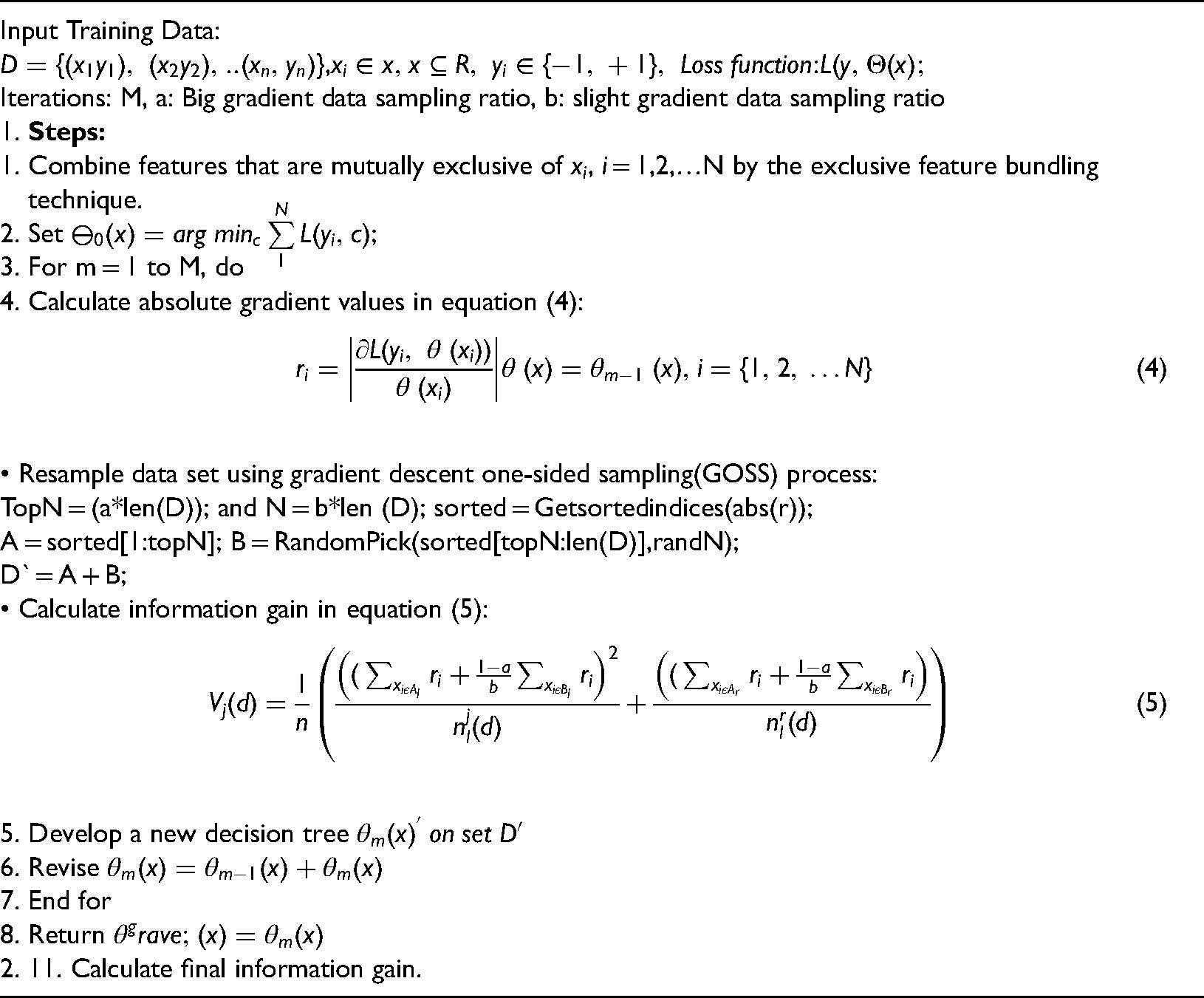
Proposed algorithm

The algorithm for the proposed hybrid LightGBM is given below:

Flow chart of proposed hybrid model

The proposed hybrid model is shown in Figure 5.

Figure 5.

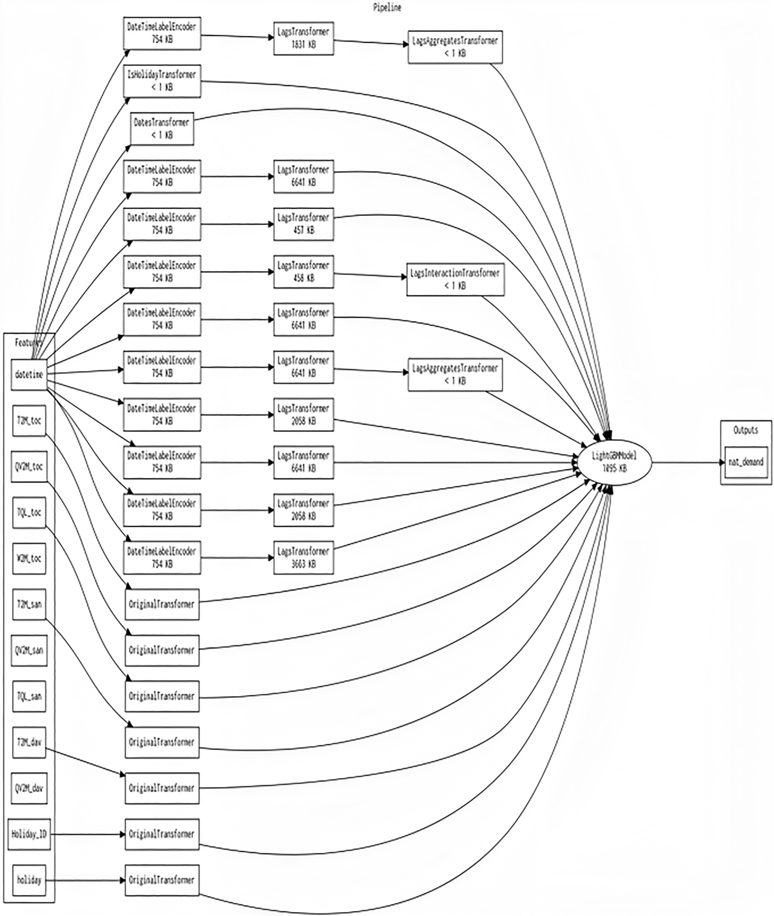
Flow of the proposed model.

The most outstanding features discovered via feature engineering iterations are the ones that are put into the final model. The target transformer specifies what transformation was used on the target column.

Results and discussion

This section covers the implementation of the proposed model, results comparisons and discussion.

Experimental setup

For this experiment, we performed the following steps to find the optimal final model, shown in Figure 6.

Figure 6.

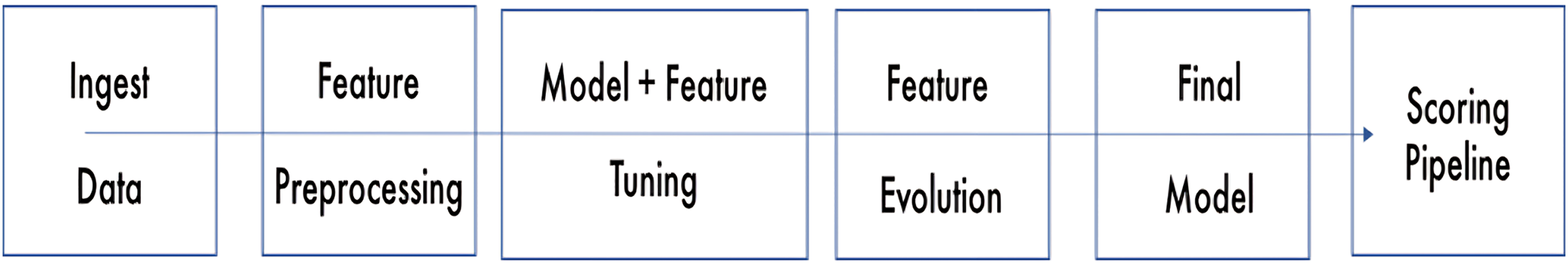
Experimental setup.

In this step, we generate features and choose hyperparameters at random. Each iteration's updates to the features are determined by a probabilistic prior that considers the relevance of the varying factors introduced in the previous iteration. Afterwards, the feature evolution stage receives the best-performing model and features. The authors trained models with variable parameters to identify the sweet spot for LightGBM, Xgboost and constant models. A genetic algorithm is employed to optimize the model's parameters and feature transformations at this point of Feature Evolution. Through developing and evaluating 67 features across 49 iterations, 774 models were trained and rated to assess designed traits better. The final model has derived from the top model after several cycles of feature engineering. No stacked ensemble was performed since a time column was given (Duan et al., 2022; Zulfiqar et al., 2022).

Experiment settings

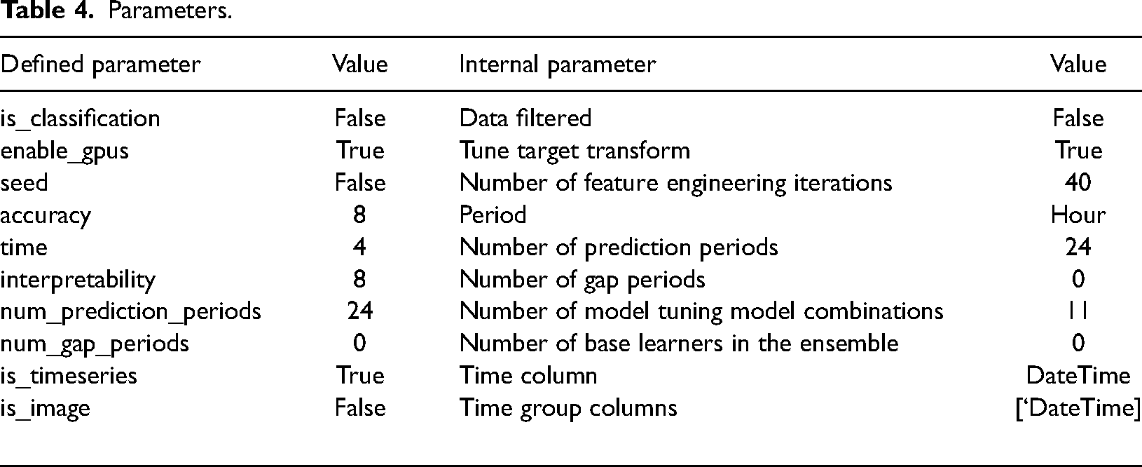
The settings selected for the experiment are specified in Table 4. The defined parameters represent the high-level parameters (Gürses-Tran et al., 2022).

Table 4.

Parameters.

Defined parameter	Value	Internal parameter	Value
is_classification	False	Data filtered	False
enable_gpus	True	Tune target transform	True
seed	False	Number of feature engineering iterations	40
accuracy	8	Period	Hour
time	4	Number of prediction periods	24
interpretability	8	Number of gap periods	0
num_prediction_periods	24	Number of model tuning model combinations	11
num_gap_periods	0	Number of base learners in the ensemble	0
is_timeseries	True	Time column	DateTime
is_image	False	Time group columns	[‘DateTime]

Model tuning

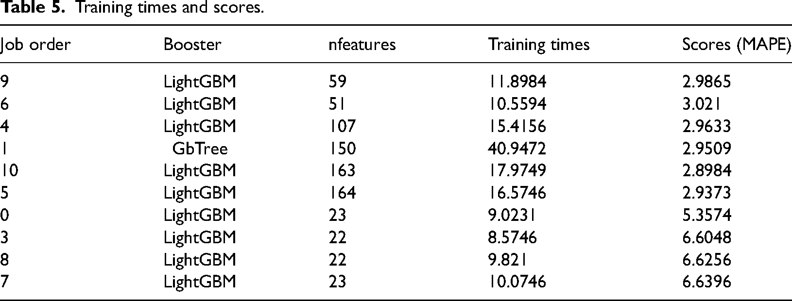
The training times and scores for the LightGBM, Xgboost and constant models (Abulibdeh et al., 2022) are listed in Table 5. Ranking by lowest score and shortest training time, the table displays the best ten parameter tuning models tested.

Table 5.

Training times and scores.

Job order	Booster	nfeatures	Training times	Scores (MAPE)
9	LightGBM	59	11.8984	2.9865
6	LightGBM	51	10.5594	3.021
4	LightGBM	107	15.4156	2.9633
1	GbTree	150	40.9472	2.9509
10	LightGBM	163	17.9749	2.8984
5	LightGBM	164	16.5746	2.9373
0	LightGBM	23	9.0231	5.3574
3	LightGBM	22	8.5746	6.6048
8	LightGBM	22	9.821	6.6256
7	LightGBM	23	10.0746	6.6396

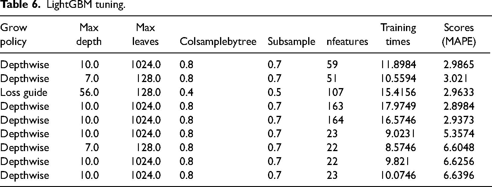
More detailed information on the parameters evaluated for each algorithm is shown in Table 6.

Table 6.

LightGBM tuning.

Grow policy	Max depth	Max leaves	Colsamplebytree	Subsample	nfeatures	Training times	Scores (MAPE)
Depthwise	10.0	1024.0	0.8	0.7	59	11.8984	2.9865
Depthwise	7.0	128.0	0.8	0.7	51	10.5594	3.021
Loss guide	56.0	128.0	0.4	0.5	107	15.4156	2.9633
Depthwise	10.0	1024.0	0.8	0.7	163	17.9749	2.8984
Depthwise	10.0	1024.0	0.8	0.7	164	16.5746	2.9373
Depthwise	10.0	1024.0	0.8	0.7	23	9.0231	5.3574
Depthwise	7.0	128.0	0.8	0.7	22	8.5746	6.6048
Depthwise	10.0	1024.0	0.8	0.7	22	9.821	6.6256
Depthwise	10.0	1024.0	0.8	0.7	23	10.0746	6.6396

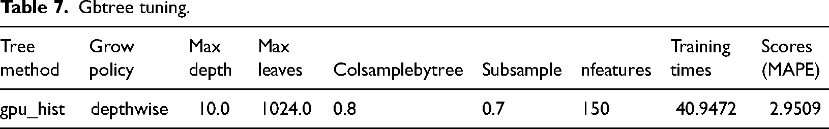
The model and feature tuning phase assesses the outcomes of trying out various algorithms, algorithm settings and features. Gbtree tuning is shown in Table 7.

Table 7.

Gbtree tuning.

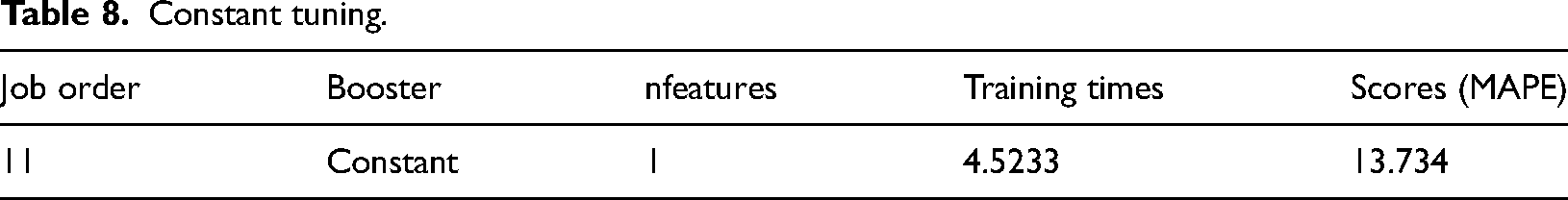
Tree method	Grow policy	Max depth	Max leaves	Colsamplebytree	Subsample	nfeatures	Training times	Scores (MAPE)
gpu_hist	depthwise	10.0	1024.0	0.8	0.7	150	40.9472	2.9509

Lightgbm, Xgboost and constant models (774) were trained at the feature evolution stage. Each model evaluated a unique subset of features shown in Table 8.

Table 8.

Constant tuning.

Job order	Booster	nfeatures	Training times	Scores (MAPE)
11	Constant	1	4.5233	13.734

An illustration of the impact of the model and feature tuning stage and the feature evolution stage on performance is shown in the graph in Figure 7.

Figure 7.

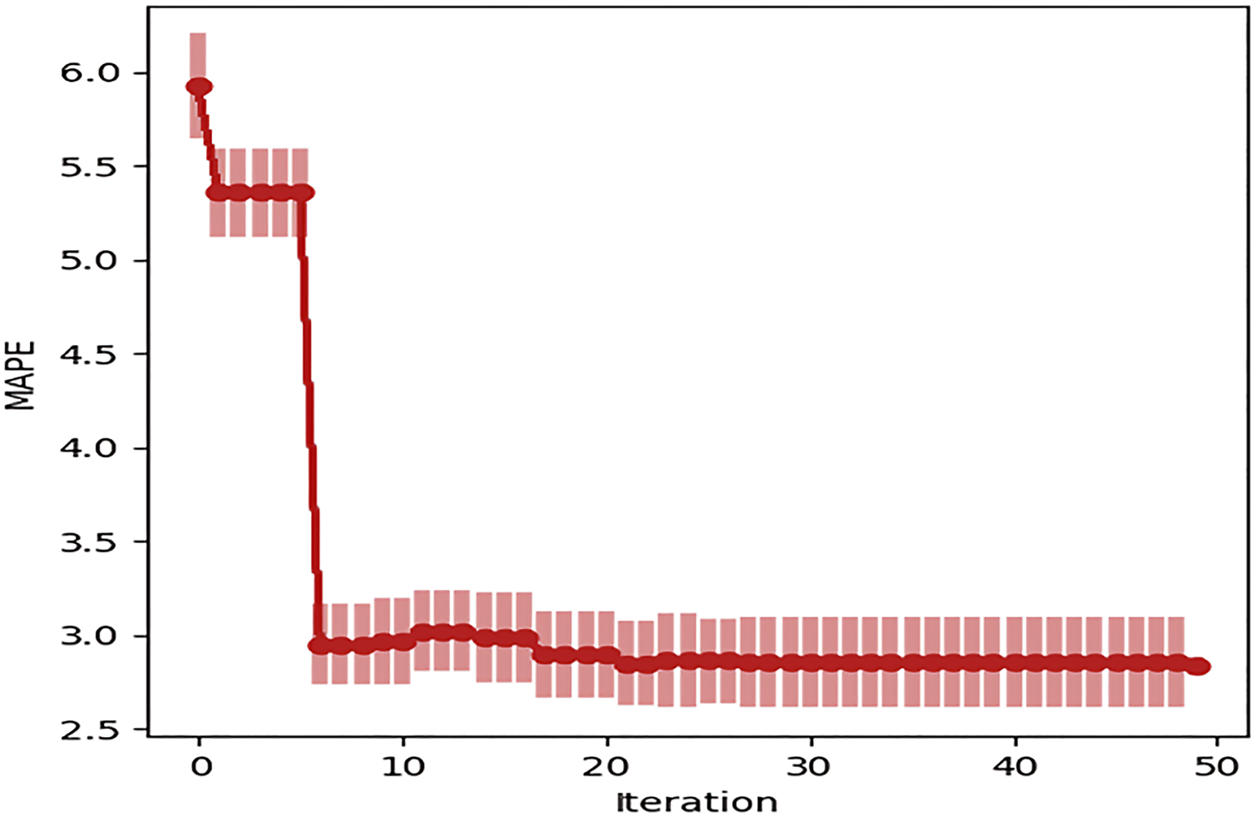
Impact of the feature tuning stage and the feature evolution.

Performance of final model

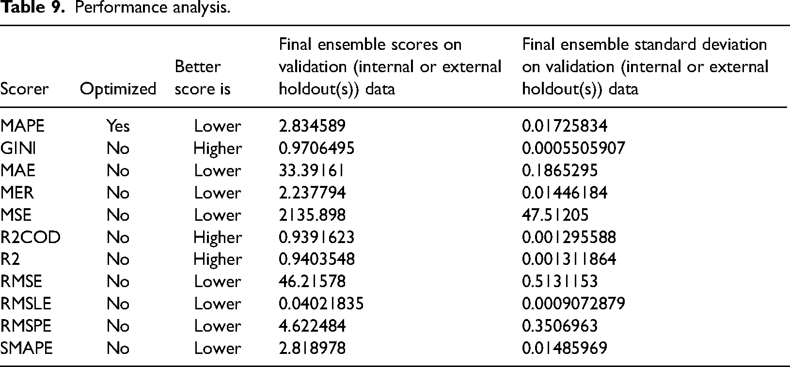
Some of the parameters measuring the performance (Pallonetto et al., 2022) of the final model are mentioned below:

MAPE: The mean absolute percentage error measures the accuracy and is given by the formula in equation (6):

MAPE = \frac{1}{m} * Σ (| A - F | / | A |) * 100

(6)

Where:

Σ – summation symbol

m – sample size

A – the actual data value

F – the forecasted data value

GINI: The Gini coefficient measures the inequality among values of a frequency distribution. It is calculated in equation (7) by:

G i n i = \frac{The Area above the Lorenz curve}{(Area above Lorenz curve + Area below Lorenz curve)}

(7)

MAE: Mean absolute error is an evaluation of errors amid paired observations. The formula for the same is in equation (8):

M A E = \frac{\sum_{i = 1}^{n} | y_{i} - x_{i} |}{n}

(8)

Where

Σ – summation symbol

n – total number of data points

y_i – prediction

x_i – true value

MER: The marketing efficiency ratio is defined as total revenue divided by total ad spending.

MSE: mean squared error compares forecasted values to actual values. It is calculated in equation (9) as:

MSE = (\frac{1}{x}) * \sum {(A - P)}^{2}

(9)

Where:

Σ – summation symbol

x – sample size

A – observed data value

P – predicted data value

RMSE: Root mean square error is a metric that tells the average value of how far apart our predicted values are from our observed values. Its formula in equation (10) is:

R M S E = \sqrt{[Σ ({(F_{i} - A_{i})}^{2}) / x]}

(10)

Where:

Σ is a symbol that means ‘sum’.

A_i is the actual ith value in the dataset

F_i is the forecasted with weight in the dataset

x is the sample size

SMAPE: Symmetric mean absolute percentage error is an accuracy evaluation of relative errors. It is calculated in equation (11) as:

SMAPE = 1 / n x Σ ((| ((F_t - A_t |) / ((F_t + A_t |))) / 2 * 100

(11)

Where A_t is the actual value, and F_t is the forecast value. Table 9 shows the performance analysis.

Table 9.

Performance analysis.

Scorer	Optimized	Better score is	Final ensemble scores on validation (internal or external holdout(s)) data	Final ensemble standard deviation on validation (internal or external holdout(s)) data
MAPE	Yes	Lower	2.834589	0.01725834
GINI	No	Higher	0.9706495	0.0005505907
MAE	No	Lower	33.39161	0.1865295
MER	No	Lower	2.237794	0.01446184
MSE	No	Lower	2135.898	47.51205
R2COD	No	Higher	0.9391623	0.001295588
R2	No	Higher	0.9403548	0.001311864
RMSE	No	Lower	46.21578	0.5131153
RMSLE	No	Lower	0.04021835	0.0009072879
RMSPE	No	Lower	4.622484	0.3506963
SMAPE	No	Lower	2.818978	0.01485969

In Figure 8, the authors have taken several input parameters like data filtered, tune target transform, number of iterations, number of models trained per iteration, early stopping rounds, number of prediction periods, number of baseline ensembles, time, number of gap periods, etc.

Figure 8.

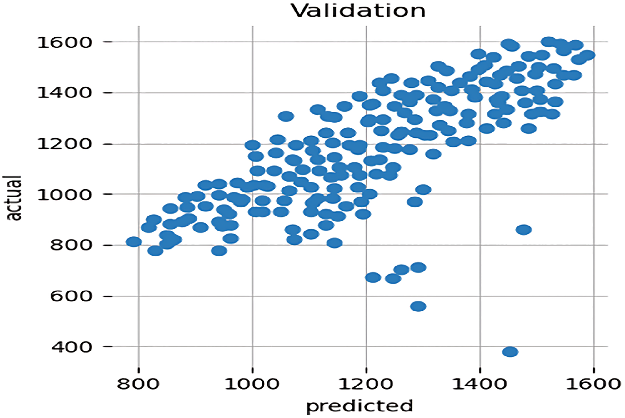
Actual versus predicted value.

Partial dependence plots

Plotting a subset of features against a set of values shows their relationship. The plots show how machine-learned response functions fluctuate with input feature values, taking into account nonlinearity and averaging out all other input features. For the first two key variables, partial dependency charts are shown. The six most relevant variables are chosen based on their significance in the original component. Figure 9 shows the Feature DateTime.

Figure 9.

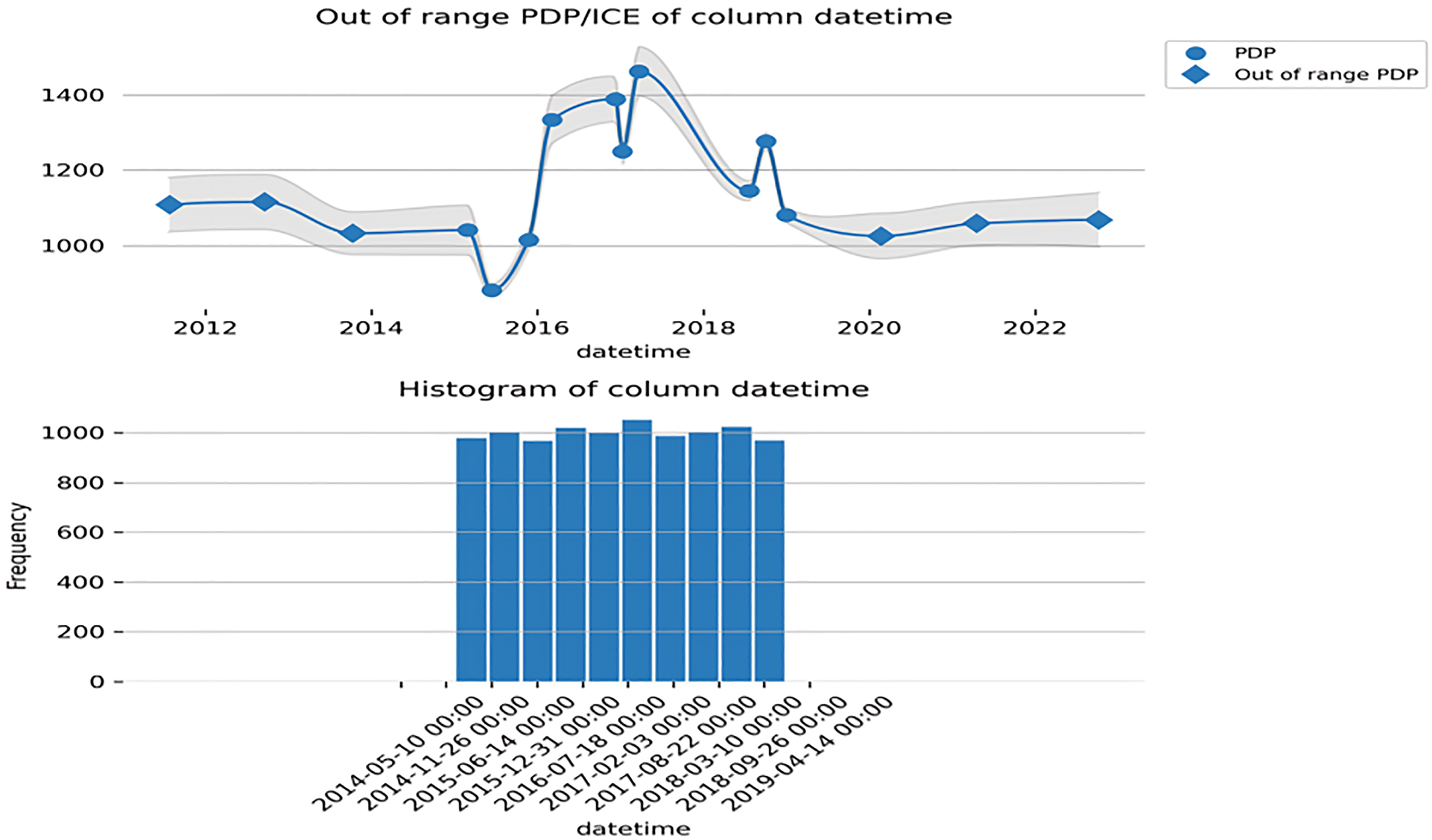
Feature DateTime.

The mean answer is displayed along the y-axis. The standard deviation is shown in Figure 10 as a shaded area (for numerical characteristics) or a shaded bar (for categorical data) above or below the mean. The diamond-shaped outliers reflect feature intervals not seen in the data, unknown category values or missing values. It is common practice to feed a model with data that spans three standard deviations in each direction from the minimum and highest training values when dealing with continuous features.

Figure 10.

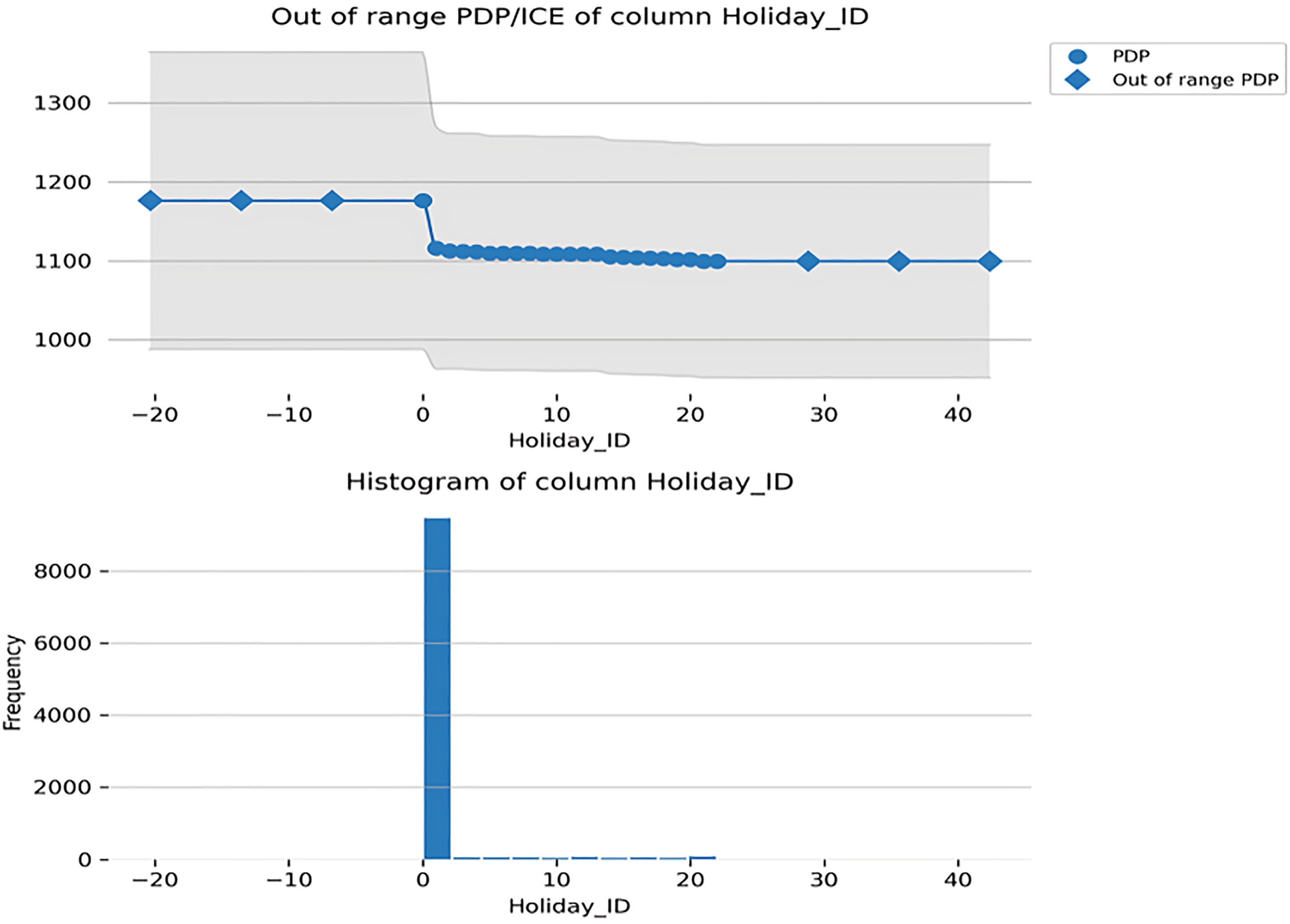
Feature Holiday_ID.

Practical implications and limitations

The hybrid model, which combines Transfer Learning with LightGBM, demonstrates substantial improvements in accuracy when compared to traditional techniques regarding short-term energy consumption forecasting in smart grids. Transfer Learning enables the algorithm to utilize learning from related categories, improving prediction efficiency effectively. The integration of LightGBM demonstrates efficacy in managing the intricate and multidimensional characteristics of smart grid statistics, leading to enhanced accuracy in load forecasting. The research examines the impacts of the hyperparameter tuning with LightGBM and identifies the most effective configurations to improve performance. The operational consequences involve enhancing energy allocation and consumption sequences, benefiting energy suppliers, grid administrators and clients.

We evaluate the results, repercussions and next steps of our hybrid model using transfer learning and LightGBM to anticipate smart grid energy loads in the near future. We compared our proposed model to baseline and state-of-the-art methods to start. We highlight that our hybrid strategy beat other methods in projected accuracy and resilience across datasets and evaluation metrics. This conversation shows how our work might improve smart grid energy load estimations’ efficiency and reliability. We explain how our hybrid model works by examining its ability to include transfer-learned global patterns and smart grid dataset-specific local characteristics. This study shows how transfer learning and LightGBM increase the model's generalization and energy usage adaptation. Here, we discuss how utility companies, grid operators and EMSs can apply our smart grid research. We can improve grid stability and energy efficiency by accurately predicting short-term energy load demand. This allows for more proactive decision-making and resource allocation. We further note that better load forecasting saves money and helps the environment. We are aware that our study relies on particular datasets and transfer learning is based on certain assumptions. To overcome these constraints, future study should investigate different transfer learning procedures, other data sources (such weather data or grid topology), and ensemble methodologies to increase predictive performance. We conclude by summarizing our research's main findings and implications, emphasizing how it promotes smart grid energy load prediction. We reiterate how important it is to keep searching for answers to improve forecasting models that can meet smart grid system expectations.

Conclusion

In this fast-paced modern age, energy predicting the future is critical to ensuring the trustable transformation of energy sources. Big data, the Internet of Things and deep learning advancements have presented investigators and related industries with numerous possibilities for supporting a stable prediction. However, due to the level of detail and accuracy of the information gathered by sensors and control devices, the variation and extremely noisy correlations posited in the statistics, and the highly complicated features that impact it, delivering reliable predictions remains a difficult task.

In this research, we developed a hybrid model for short-term energy load prediction based on transfer learning with LightGBM for smart grids. This research utilizes a real-time Panama dataset. The proposed model first applies data pre-processing. This phase eliminates the missing values and extracts the required features. The second phase uses substantial transfer learning with LightGBM with hyperparameters. Initially, the proposed model decomposes the time series of load demand. Second, a correlation analysis between the system load and exogenous input factors is implemented to improve the accuracy of the peak load forecast. Third, the appropriate model makes predictions for both parts independently. Final projections are obtained by summing the estimates of each subcomponent. Data on energy use from the Panama power markets are used to test the validity of the suggested model. The proposed approach enhances forecasting accuracy according to all case study outcomes. The hybrid model can capture the many features of the electrical load because it takes advantage of the strengths of both the traditional and the modern models.

Consequently, the suggested model may deliver reliable, consistent and improved forecasts. For future electrical load forecasting, sophisticated models can be employed to choose appropriate input factors. In addition, the hybrid model may be expanded to include other future influencing elements, such as customer information about incentive-based demand response programs and uncertainty from the integration of distributed renewable energy sources. This framework can potentially improve Panama's short-term scheduling and operations for generating. The research proposes future directions to overcome challenges, such as expanding the model to make predictions over extended periods and integrating more data sources to comprehend energy load patterns better. In summary, the hybrid model offers a new and efficient solution for enhancing short-term energy load forecasting in smart grids, potentially improving grid management and optimizing resource utilization.

Footnotes

Acknowledgements

We would like to acknowledge all who have directly/indirectly supported this research.

Author contributions

SS was responsible for validation, software, data curation and writing – original draft. MD was responsible for conceptualization, writing – original draft. ST was responsible for writing – original draft, visualization. YKS & NF were responsible for writing – review & editing. ST was responsible for formal analysis. NN was responsible for writing – original draft, resources. The authors read and approved the final manuscript.

Data availability statement

The dataset will be available with the corresponding author based on individual requests.

Declaration of conflicting interests

The authors declared no potential conflicts of interest with respect to the research, authorship, and/or publication of this article.

Funding

The authors received no financial support for the research, authorship, and/or publication of this article.

ORCID iD

Nasratullah Nuristani

References

Abdulrahman

Ibrahim

Gital

, et al. (2021) A review on deep learning with focus on deep recurrent neural network for electricity forecasting in residential building. Procedia Computer Science 193: 141–154.

Abulibdeh

Zaidan

Jabbar

(2022) The impact of COVID-19 pandemic on electricity consumption and electricity demand forecasting accuracy: Empirical evidence from the state of Qatar. Energy Strategy Reviews 44(October): 100980.

Azeem

Ismail

Jameel

, et al. (2021) Electrical load forecasting models for different generation modalities: A review. IEEE Access 9: 142239–142263.

Becirovic

Cosovic

(2016) Machine learning techniques for short-term load forecasting. 4th International Symposium on Environment-Friendly Energies and Applications EFEA 2016: 8–11.

Chen

Fang

Zhou

, et al. (2021) Electricity short-term load computer intelligent forecasting model under robust extreme learning machine and numerical simulation. Proceedings of 2021 IEEE International Conference on Emergency Science and Information Technology, ICESIT 2021 3(3): 651–656.

Chung

Yoo

(2022) District heater load forecasting based on machine learning and parallel CNN-LSTM attention. Energy 246: 123350.

Dataset (2023) “Electrical Grid Stability Simulated Dataset”, access on 5th Jan 2023, collected from UCI Machine Learning Repository, https://archive.ics.uci.edu/dataset/471/electrical + grid + stability + simulated + data.

Deng

Wang

, et al. (2019) Multi-scale convolutional neural network with time-cognition for multi-step short-term load forecasting. IEEE Access 7: 88058–88071.

De Vilmarest

Goude

(2022) State-space models for online post-Covid electricity load forecasting competition. IEEE Open Access Journal of Power and Energy 9(June): 192–201.

10.

Dokur

Erdogan

Salari

, et al. (2022) Offshore wind speed short-term forecasting based on a hybrid method: Swarm decomposition and meta-extreme learning machine. Energy 248: 123595.

11.

Duan

Hou

Fang

, et al. (2022) A novel electricity consumption forecasting model based on kernel extreme learning machine-with generalized maximum correntropy criterion. Energy Reports 8: 10113–10124.

12.

Dudek

Pełka

(2021) Pattern similarity-based machine learning methods for mid-term load forecasting: A comparative study. Applied Soft Computing 104: 107223.

13.

Gilanifar

Wang

Sriram

LMK

, et al. (2020) Multitask Bayesian spatiotemporal Gaussian processes for short-term load forecasting. IEEE Transactions on Industrial Electronics 67(6): 5132–5143.

14.

Gürses-Tran

Körner

Monti

(2022) Introducing explainability in sequence-to-sequence learning for short-term load forecasting. Electric Power Systems Research 212(March): 108366.

15.

Hadjout

Torres

Troncoso

, et al. (2022) Electricity consumption forecasting based on ensemble deep learning with application to the Algerian market. Energy 243: 123060.

16.

Han

Yan

(2021) A task-based day-ahead load forecasting model for stochastic economic dispatch. IEEE Transactions on Power Systems 36(6): 5294–5304.

17.

Huang

Wang

, et al. (2020) Incorporating load fluctuation in feature importance profile clustering for day-ahead aggregated residential load forecasting. IEEE Access 8: 25198–25209.

18.

Jawad

Nadeem

MSA

Shim

, et al. (2020) Machine learning based cost effective electricity load forecasting model using correlated meteorological parameters. IEEE Access 8: 146847–146864.

19.

Jiang

Wang

, et al. (2021) Hybrid multitask multi-information fusion deep learning for household short-term load forecasting. IEEE Transactions on Smart Grid 12(6): 5362–5372.

20.

Jiang

Zhu

, et al. (2018) Electricity power load forecast via long short-term memory recurrent neural networks. Proceedings - 2018 4th Annual International Conference on Network and Information Systems for Computers ICNISC 2018: 265–268.

21.

Jiang

Zhu

, et al. (2021) A bottom-up method for probabilistic short-term load forecasting based on Medium voltage load patterns. IEEE Access 9(Mv): 76551–76563.

22.

Kong

Zhang

, et al. (2020) Multimodal feature extraction and fusion deep neural networks for short-term load forecasting. IEEE Access 8: 185373–185383.

23.

Liu

Nowotarski

Hong

, et al. (2017) Probabilistic load forecasting via quantile regression averaging on sister forecasts. IEEE Transactions on Smart Grid 8(2): 730–737.

24.

Mamun

Sohel

Mohammad

, et al. (2020) A comprehensive review of the load forecasting techniques using single and hybrid predictive models. IEEE Access 8: 134911–134939.

25.

Marwala

Twala

(2018) Electricity load forecasting using an ensemble of optimally pruned and basic extreme learning machines. 2017 9th IEEE-GCC Conference and Exhibition GCCCE 2017: 1–6.

26.

McHugh

Coleman

Kerr

(2022) Hourly electricity price forecasting with NARMAX. Machine Learning with Applications 9(August 2021): 100383.

27.

Mousa

Aghaei

Afrasiabi

, et al. (2022) Probability density function forecasting of electricity price: Deep gabor convolutional mixture network. Electric Power Systems Research 213(February): 108325.

28.

Naz

Javaid

Khalid

, et al. (2020) Electric load forecasting using EEMD and machine learning techniques. 2020 International Wireless Communications and Mobile Computing, IWCMC 2020: 2124–2127.

29.

Obst

De Vilmarest

Goude

(2021) Adaptive methods for short-term electricity load forecasting during COVID-19 lockdown in France. IEEE Transactions on Power Systems 36(5): 4754–4763.

30.

Ouyang

, et al. (2019) Modelling and forecasting short-term power load with copula model and deep belief network. IEEE Transactions on Emerging Topics in Computational Intelligence 3(2): 127–136.

31.

Pallonetto

Jin

Mangina

(2022) Forecast electricity demand in commercial building with machine learning models to enable demand response programs. Energy and AI 7(July 2021): 100121.

32.

Phyo

Jeenanunta

(2021) Daily load forecasting based on a combination of classification and regression tree and deep belief network. IEEE Access 9: 152226–152242.

33.

Wan

Cao

Lee

, et al. (2021) An adaptive ensemble data-driven approach for nonparametric probabilistic forecasting of electricity load. IEEE Transactions on Smart Grid 12(6): 5396–5408.

34.

Xuan

Zhu

, et al. (2021) Multi-Model fusion, short-term load forecasting, based on random forest feature selection and hybrid neural network. IEEE Access 9: 69002–69009.

35.

Zhao

Wang

Zhang

(2019) Day-Ahead hierarchical probabilistic load forecasting with linear quantile regression and empirical copulas. IEEE Access 7: 80969–80979.

36.

Zhou

Hao

, et al. (2020) An electricity load forecasting model for integrated energy system based on BiGAN and transfer learning. Energy Reports 6: 3446–3461.

37.

Ziel

(2022) Smoothed bernstein online aggregation for short-term load forecasting in IEEE DataPort competition on day-ahead electricity demand forecasting: Post-COVID paradigm. IEEE Open Access Journal of Power and Energy 9(June): 202–212.

38.

Zulfiqar

Kamran

Rasheed

, et al. (2022) Hyperparameter optimization of support vector machine using adaptive differential evolution for electricity load forecasting. Energy Reports 8: 13333–13352.

A transfer learning-based hybrid model with LightGBM for smart grid short-term energy load prediction

Abstract

Keywords

Introduction

Demand and utilities of energy

Analysis of anticipated demand and supply

Related work

Material and methods

Dataset

Shapley values

Gradient boosted machines

Architecture

Proposed hybrid model

Proposed algorithm

Flow chart of proposed hybrid model

Results and discussion

Experimental setup

Experiment settings

Model tuning

Performance of final model

Partial dependence plots

Practical implications and limitations

Conclusion

Footnotes

Acknowledgements

Author contributions

Data availability statement

Declaration of conflicting interests

Funding

ORCID iD

References