Sage Journals: Discover world-class research

Abstract

In order to accurately predict reservoirs with similar physical properties between sandstone and surrounding rocks, this study takes Carboniferous-Permian system in southeastern Ordos Basin as an example, and puts forward a multi-attribute probabilistic neural network prediction method based on acoustic time difference compaction correction. Firstly, the time-frequency analysis method is used to divide the frequency of the original acoustic time difference curve, and the low-frequency long-trend correction of all wells is carried out based on the low-frequency components of standard wells. Then, it is frequency-divided and fused with the original high-frequency components to form new acoustic time difference data, and the long-term trend decompaction correction of acoustic time difference is completed, so that the overlapping area of acoustic time difference between reservoir and surrounding rock is reduced. Multi-attribute probabilistic neural network is an algorithm based on sampling points, before reservoir prediction, inversion parameters must be optimized to save calculation time and reduce prediction error. There is a high correlation between longitudinal velocity and lithologic change trend on the inversion profile of sound velocity. The comparison results of various inversions show that the velocity profile of multi-attribute probabilistic neural network has the highest coincidence rate and high resolution with the velocity curve of logging acoustic wave. The example shows that this method has high accuracy in predicting reservoir thickness, especially for the strata with little difference in physical properties between reservoir and surrounding rock.

Keywords

decompaction correction multi-attribute probabilistic neural network reservoir prediction attribute optimization

Introduction

Acoustic transit time data is often used to identify reservoirs and is the key to connecting well logging and seismic data (Withers, 1992; Hampson et al., 2001; Du et al., 2010; Ashraf et al., 2019). Seismic waves are affected by physical properties of rocks when passing through formations in the subsurface. Petrophysical evaluation of a formation using petrophysical logs and core data plays an important role in determining the formation and the characteristics of the reservoir (Abdideh et al., 2019, 2020; Teymori et al., 2020). In general, the acoustic transit time of the reservoir is different from that of the surrounding rock, which provides a reliable basis for seismic interpretation. If the geological factors are complex and the reservoir is tightened (Liu et al., 2014; Guo et al., 2021), the difference between the acoustic time difference or the density and the surrounding rock is slight, which will seriously affect the accuracy of seismic reservoir prediction. Suppose the influence of compaction on the acoustic transit time is weakened. In that case, the acoustic transit time difference between the reservoir and the surrounding rock will become more prominent, which is beneficial to the subsequent seismic inversion processing and analysis (Perrier and Quilbier, 1974; Qi and Yang, 2001). Comprehensive rock physics characterization analysis, deep machine learning and data-driven methods are also used to modify acoustic logging and improve its application to reservoir inversion. The usual sonic decompaction correction method uses statistical methods to establish the porosity-depth function of the stratum. It then decompresses to the principle that the skeleton volume remains unchanged correction (Wu, 1989; Li et al., 2000; Yang and Qi, 2003; Abdideh and Dastyaft, 2022). This method is relatively rigorous in theory, but the operation process is complicated, with many influencing factors. It is often impossible to obtain accurate primary porosity values and proper porosity-depth functions. Acoustic frequency division reconstruction is a solution to the above problems. The method is to fuse and reconstruct the high-frequency components of the logging curve sensitive to lithology and the original low-frequency components of the acoustic wave and then use the reconstructed curve for reservoir inversion, but this plan lacks strong geophysical theoretical support (Zhang et al., 2005;Yang and Qiao, 2021). Therefore, for the prediction of tight reservoirs, this study proposes a decompression correction method for the long trend of acoustic transit time. The standard well is selected to uniformly correct the low-frequency component of the acoustic wave in this area. Then it is fused with the original high-frequency element to form a new acoustic time difference curve.

Artificial intelligence is constantly changing the oil and gas exploration and development industry. There is still a particular gap between large-scale seismic data processing and interpretation technology and the actual production demand. Advanced AI algorithms must be developed to improve data quality and tap data potential. As an essential branch of artificial intelligence, the neural network has become a very effective mathematical analysis tool (Feng, 2020; Sircar et al., 2021). In particular, the probabilistic neural network, popular in recent years, has been widely and successfully applied in oil and gas seismic inversion (McCormack, 1991; Emilson and Alexandre, 2010; Maurya and Singh, 2018; Lee et al., 2022). The advantage of the probabilistic neural network (PNN) is that it can stably converge to the Bayesian optimization solution without multiple complete calculations (Roth and Tarantola, 1994; Walls et al., 2002; Triveni and Rima, 2019). In order to reveal the underground reservoir lithology, structure, and physical properties, seismic inversion often depends on massive seismic, logging, and core data, trying to optimize the nonlinear function between seismic data and reservoir parameters. Conventional seismic reservoir prediction is mostly based on conventional logging data combined with seismic inversion or combining geological modeling to predict the distribution of favorable reservoirs. The theoretical basis is that the petrophysical characteristics of the reservoir are significantly different from the surrounding rocks (Ashraf et al., 2019; Anees et al., 2022a, 2022b). The acoustic time difference corrected by mudstone decompaction combined with the multi-attribute probabilistic neural network can realize the accuracy inversion of underground reservoir characteristics by continuously learning from abundant sample data and then fitting complex nonlinear functions (Masters, 1994; Xie et al., 2015; Yazmyradova et al., 2021). After decompressing correction, the overlapping area of the acoustic time difference between the reservoir and surrounding rock is reduced, and the neural network seismic inversion based on this has high resolution.

Under the influence of compaction, the rock structure of the formation changes significantly (Liu et al., 2014). The physical properties of the reservoir deteriorate, the pore space shrinks, and the reservoir becomes tight. It is challenging to distinguish reservoirs effectively using the original acoustic velocity characteristics for formations with similar acoustic velocity characteristics of reservoirs and surrounding rocks. This type of reservoir makes the acoustic velocity-based reservoir seismic inversion without a reliable geophysical basis. This study takes Permian and Carboniferous in the southeastern Ordos Basin as an example to discuss the accurate prediction method for solving such reservoirs (Figure 1).

Figure 1.

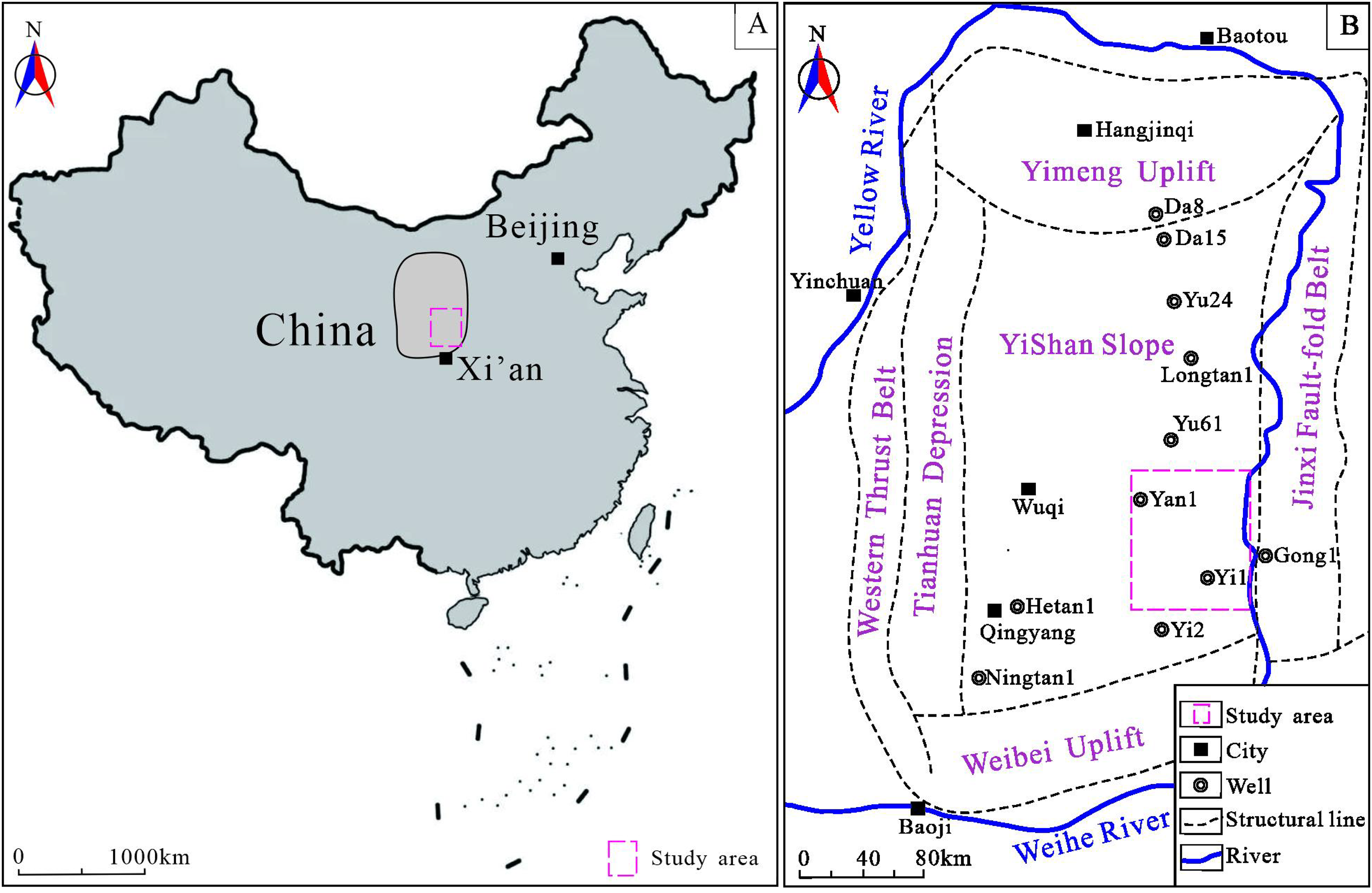
Location and structure of the Ordos Basin.

Geological setting

The Ordos Basin was formed in the Palaeozoic, inherited and developed in the Mesozoic and Cenozoic (Sun et al., 2009; Liu et al., 2009). It is a typical multisedimentary cycle cratonic basin, which evolved as a large-scale intracontinental sedimentary basin during the Indonesian tectonic movement ( Sun et al., 2009). The late Paleozoic strata in the study area are a set of marine continental transitional clastic rock series, and the total thickness of sedimentary rock is about 700 m. The important strata in this study are the Carboniferous Benxi, Shihezi, Shanxi formations and the Permian Taiyuan formation. Among these, the He8 member and Shanxi formation is the most important gas-producing interval (Figure 2; Liu et al., 2009; Zhu et al., 2021).

Figure 2.

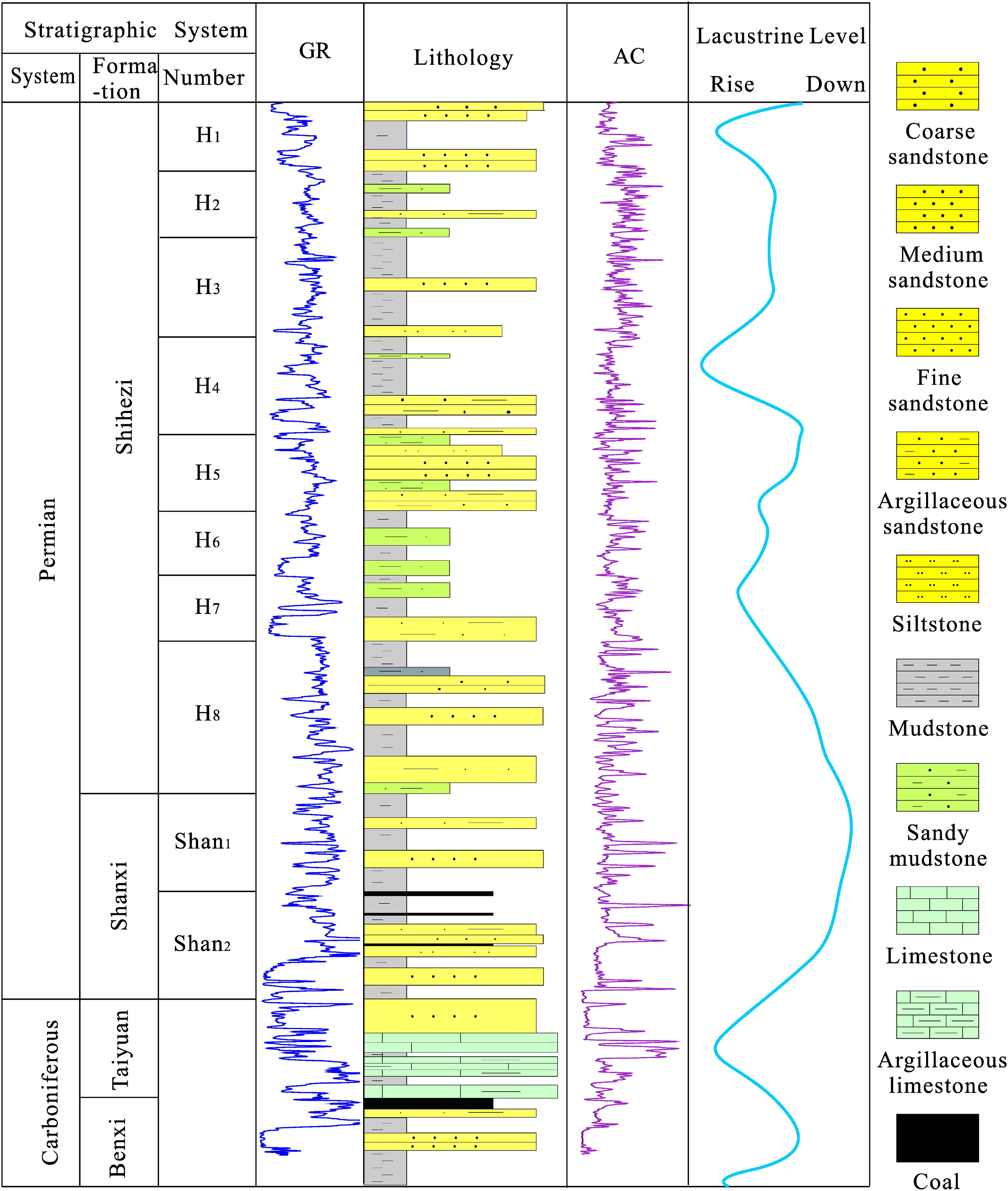
Stratigraphic characteristics and sedimentary cycles of carboniferous-permian strata in Ordos Basin.

Data and methods

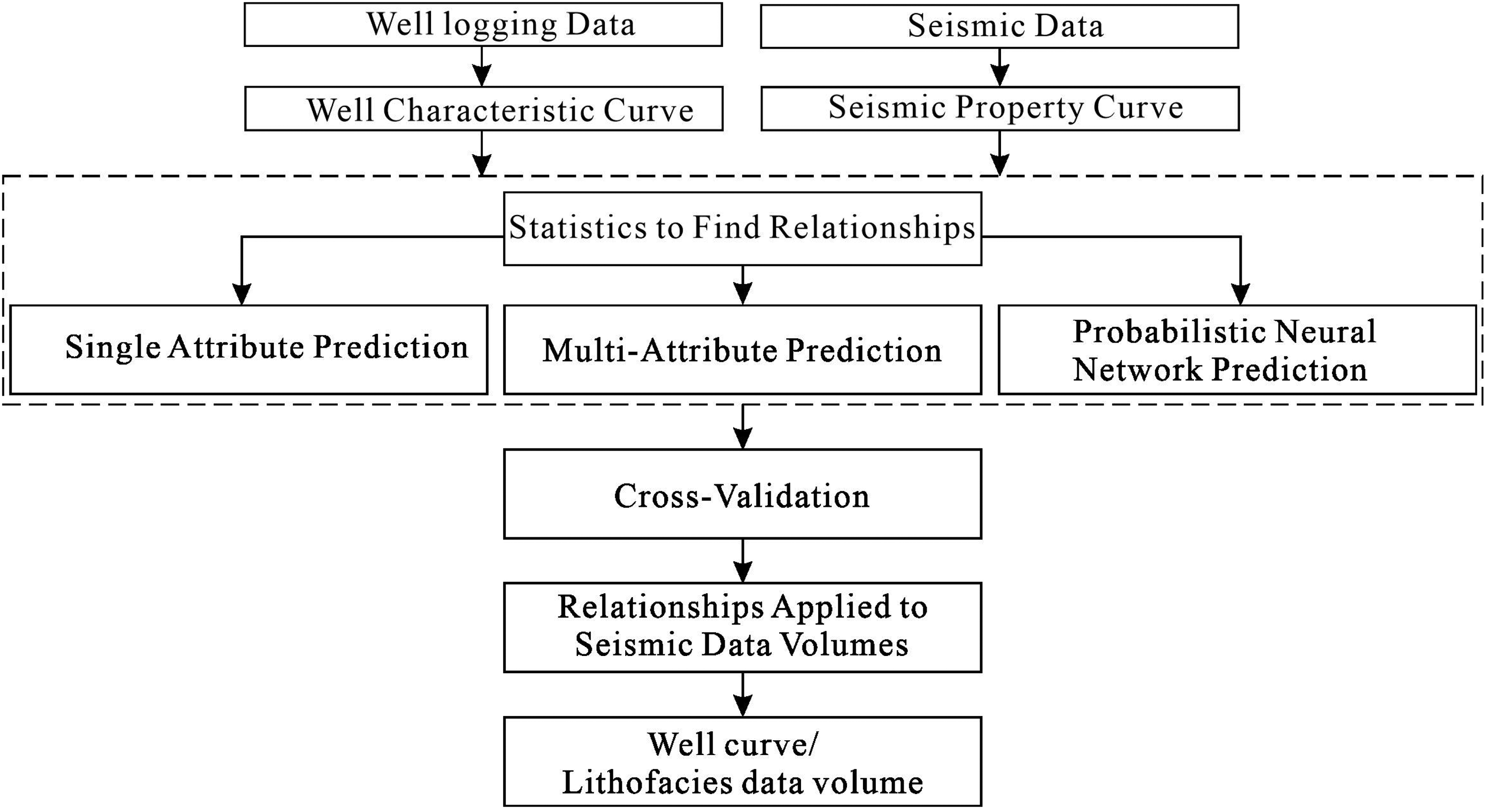
It is difficult to distinguish the characteristics of the acoustic time difference between some reservoirs and surrounding rocks (Trappe and Hellmich, 1995; Nikravesh and Aminzadeh., 2001; Lai et al., 2020). For such reservoirs, this study integrates sound velocity decompression correction and multi-attribute neural network inversion methods to improve reservoir prediction accuracy (Figure 3). This study used 96 exploratory wells, 115 2D seismic lines, and more than 400 square kilometers of 3D seismic data. Firstly, selected standard wells were used to uniformly correct the low-frequency components of acoustic waves in this area and then fuse them with the original high-frequency components to form a new acoustic time difference curve. Secondly, logging curves and seismic data according to the data of known wells were analyzed and a data volume was extracted using nonlinear regression and artificial neural network technology, to find out the characteristic relationship between seismic attributes and logging characteristics. Thirdly, the neural network applies this high-correlation mapping relationship to the actual seismic data to complete the inversion of neural network logging features.

Figure 3.

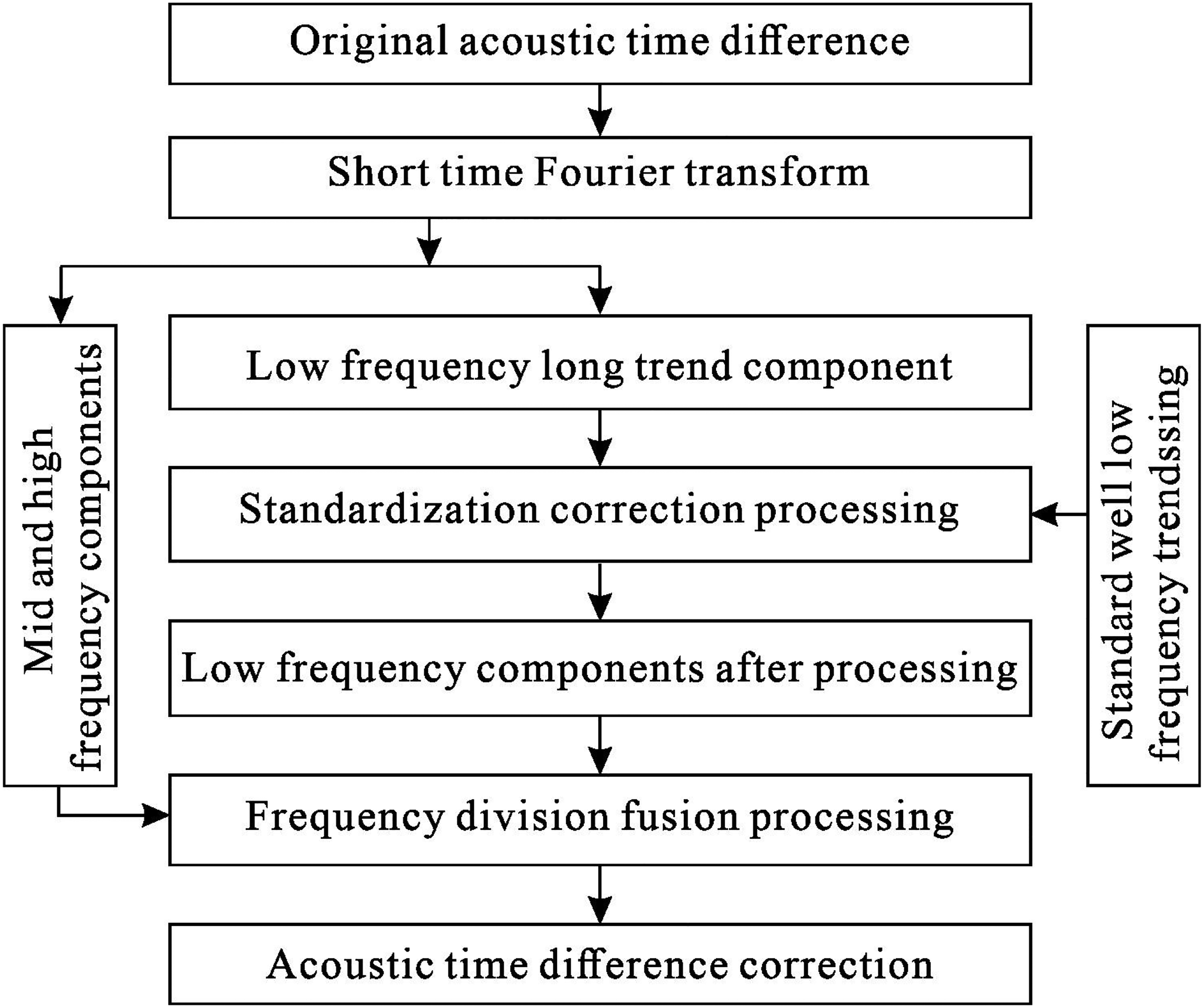
Technical process of sonic time difference long trend decompaction correction.

Acoustic wavelength trend decompaction correction

The cross-plot method analyzed the sound velocity distribution characteristics corresponding to the lithology sampling points. Unlike seismic data, time-frequency analysis of acoustic travel time curves does not require overly complex transformations. The short-time Fourier transform method is used here, and its expression is:

STFT (t, f) = \int_{- \infty}^{\infty} e^{- i ω t} f (τ) g (t - τ) d t

(1)

f(t) is the input signal, t is the time; g(t-τ) is the symmetrical time window function; τ is the time shift; ω is the angular frequency; e is a natural constant; i is an imaginary unit.

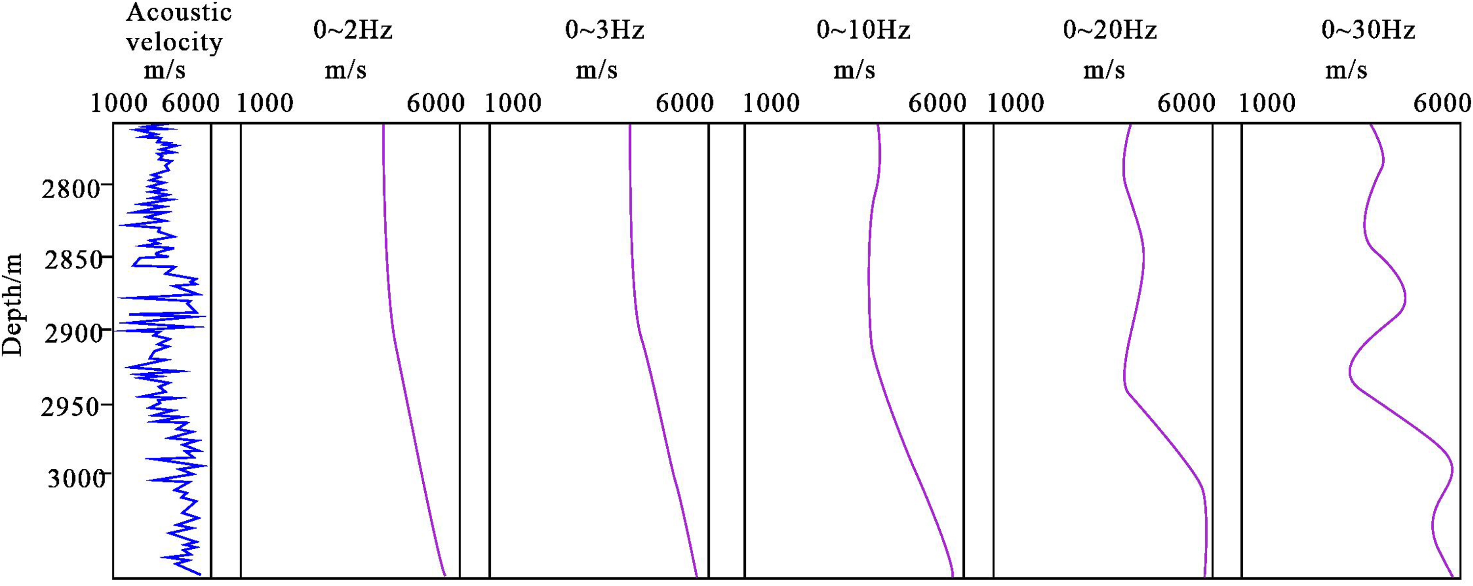
The separation curve of the low-frequency component and high-frequency component of the acoustic velocity shows that the low-frequency component changes gently. In contrast, the high-frequency component exhibits frequent jitter and spikes, which reflect the stratigraphic structure (Figure 3). On the basis of the time-frequency analysis of the acoustic transit time curve, through the spectrum scanning of the signal and referring to the current research results (Soleimani, 2013; Zhang et al., 2015), the signal with frequency components below 2 Hz is finally defined as the long trend of low-frequency acoustic transit time components (Figure 4).

Figure 4.

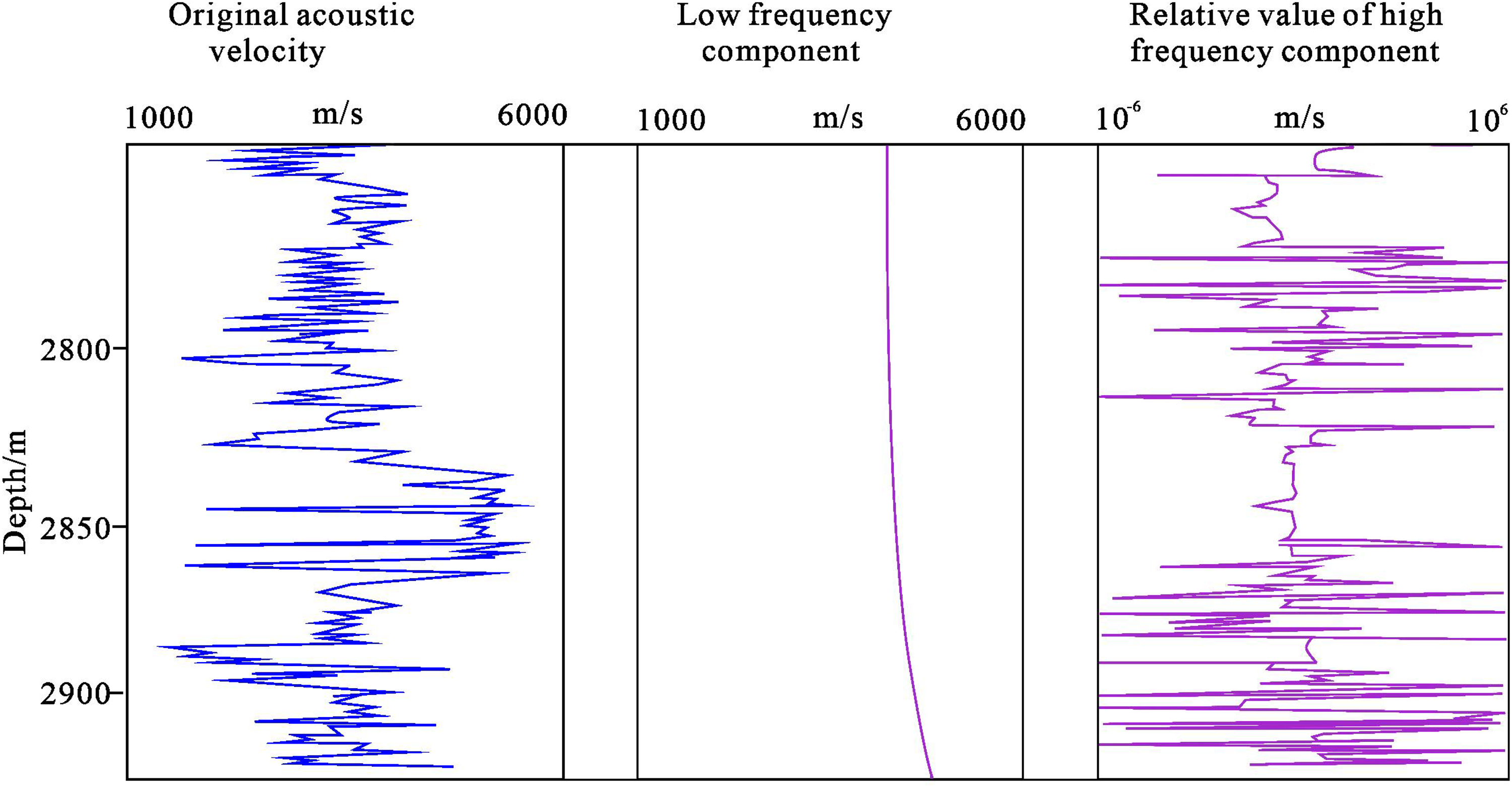
Separation curve of the low and high-frequency components of acoustic velocity (Well 140).

Take the acoustic transit time curve that can clearly distinguish the lithology as the standard well curve and perform time-frequency analysis on all wells acoustic transit time curves. Taking the low-frequency and long-trend components of the acoustic transit time of standard wells as a reference, the low-frequency components of acoustic transit time and long trend of all wells are standardized. The standardization process uses the frequency distribution histogram method to determine the probability peak of the low-frequency component distribution in the standard well. It uses the probability peak velocity difference to complete the low-frequency component correction of other wells (Figure 5). The corrected low-frequency and original mid and high-frequency components are superimposed in the frequency domain. Then the inverse Fourier transform is used to complete the frequency division reconstruction and decompression correction through the inverse Fourier transform in time and deep transform. A new acoustic time difference curve is obtained (Figure 6).

\tilde{f} (t) = \frac{1}{2 π} \int_{- \infty}^{\infty} e^{i ω t} F (ω) d ω

(2)

Figure 5.

Characteristics of low-frequency components of acoustic velocity (Well 140).

Figure 6.

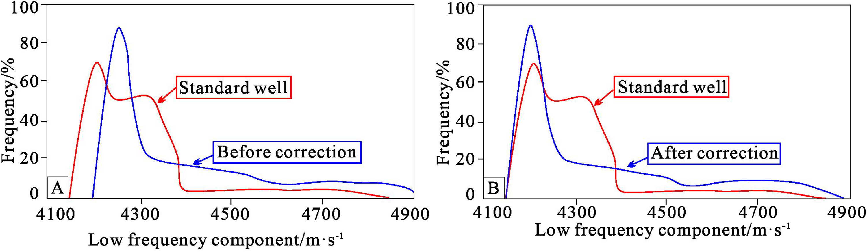
Frequency distribution of low-frequency component of acoustic velocity.

F(ω) is the frequency spectrum, $\tilde{f} (t)$ is the output signal.

Multi-attribute probabilistic neural network modeling (MPNN)

The prediction results of existing neural network seismic reflection models are often unstable, and multiple results may appear in multiple predictions, so it is difficult to evaluate the accuracy of the prediction results. Moreover, the predicted values only represent different reflection categories, and there is no corresponding geological indication and meaning (Meldahl et al., 1999; Ding et al., 2018). Probabilistic neural network (PNN) was first proposed by the Specht in 1990. PNN is a neural network with strong generalization ability based on probability density functions which consists of input layer, mode layer, summation layer and output layer. PNN introduces convolution factor, predicts the value of a point on the logging curve through the weighted average of a group of sampling points on each attribute, and establishes the correlation between multiple sampling points adjacent to the attribute and logging data (Daniel, 2001; Ma et al., 2004). In Figure 7, X = [x1, x2, …xm] is the input M-dimensional vector, and m is the number of neurons in the input layer. Y = [y1, y2, …, ym] is the output vector, and l is the number of types to be recognized.

Figure 7.

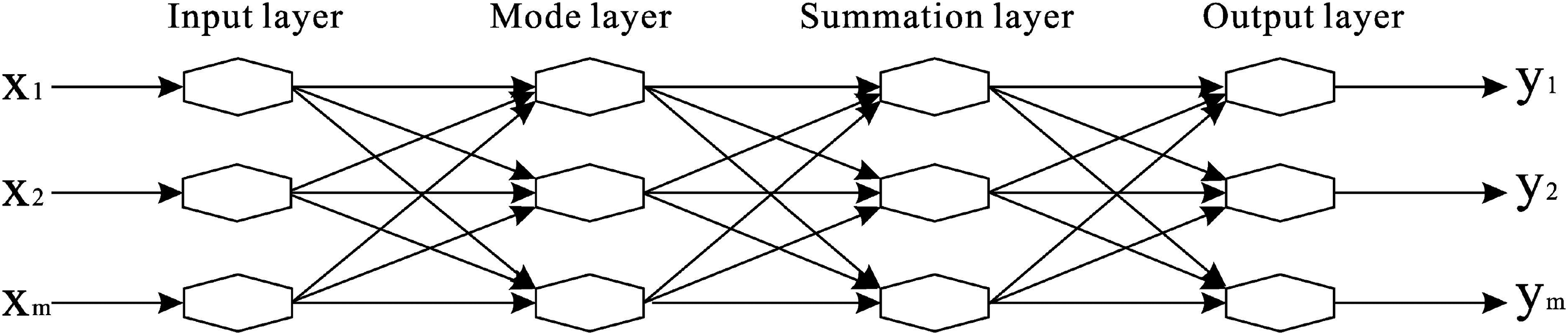
Probabilistic neural network (PNN) architecture.

Probabilistic neural network prediction method based on logging geological information constraint can supervise seismic attribute optimization and sensitivity analysis, and improve the prediction accuracy of seismic reflection mode (Gong et al., 2009; Ding et al., 2018). The combination of seismic attributes selected by sound velocity inversion is used as the input of the neural network. The decompression-corrected acoustic velocity of the existing well is used as the neural network output. Firstly, using the data of known wells and the input seismic attributes as training data, the neural network is trained to establish a nonlinear model between the seismic attributes and the logging acoustic velocity. When the error reaches a reasonable range, the neural network model is considered to be established. At the same time, the weights and thresholds at the hidden layer nodes in the neural network are also obtained. The established model is then applied to all seismic data to complete the acoustic velocity inversion for the entire study area (Figure 8).

Figure 8.

Multi-attribute probabilistic neural network inversion processing flow chart.

Seismic attribute optimization. The decompression correction method was used to correct the decompression curve of the acoustic wave time difference using the acoustic wavelength trend decompression correction method, and the decompression acoustic wave propagation velocity was obtained. The seismic attributes were extracted, and the combination of seismic attributes was optimized by stepwise regression analysis. Multi-attribute fitting is carried out by using the acoustic wave curve corrected forde-compaction in well 228. According to the verification error analysis, the convolution factor is 7, and the fitting effect of 9 seismic attributes is good. Fitting with the neural network, the correlation coefficient is 93% and the average error is 298 m/s (Table 1). Taking the porosity curve of well 163 as an example, multi-attribute fitting is carried out. According to the verification error analysis, the convolution factor is 11, and the fitting effect of 6 seismic attributes is good. Using neural network fitting, the correlation coefficient is 90% and the average error is 0.4 (Table 1).

Table 1.

List of the seismic multi-attribute combination.

Number	Target	Final Attribute	Training Error	Validation Error
1	Sqrt(P-wave)	Filter 5/10–15/20	520.8795	533.0926
2	Sqrt(P-wave)	Sqrt(1)	504.2453	521.7154
3	Sqrt(P-wave)	Quadrature Trace	493.2239	510.4948
4	Sqrt(P-wave)	Filter 15/20–25/30	483.6744	504.0542
5	Sqrt(P-wave)	Filter 55/60–65/70	476.8825	499.0920
6	Sqrt(P-wave)	Apparent polarity	470.8975	490.9462
7	Sqrt(P-wave)	Instantaneous frequency	467.8683	490.4228
8	Sqrt(P-wave)	Instantaneous phase	466.6453	490.2331
9	Sqrt(P-wave)	Integrated absolute amplitude	464.9752	489.5485
11	Log(Porosity)	Instantaneous frequency	1.3149	1.4445
12	Log(Porosity)	Log(33)	1.2362	1.4283
13	Log(Porosity)	Amplitude weighted cosine phase	1.1777	1.3889
14	Log(Porosity)	Filter 45/50–55/60	1.1531	1.3645
15	Log(Porosity)	Dominant frequency	1.1320	1.3711
16	Log(Porosity)	Average frequency	1.1013	1.2936

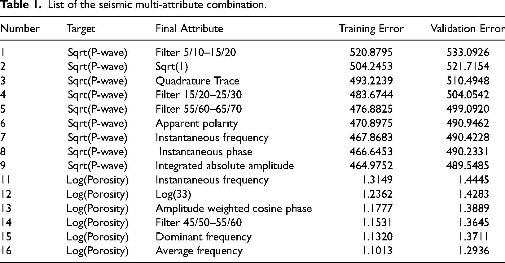
The training error is still decreasing through cross-validation when the number of seismic attributes increases to 9. Still, the validation error increases and the target curve (acoustic transit time) begins to overfit, so the optimal number of seismic attributes is determined to be set to 9. The input parameters of this neural network modeling include: instantaneous frequency, absolute amplitude of channel integral, 35/40–45/50 filter slice, amplitude weighted cosine phase, original amplitude, dominant frequency, second differential amplitude, apparent polarity, average frequency, seismic properties, the target curve is the decompaction sonic time difference.

Key parameters of the probability network. The key parameters of a probabilistic neural network mainly include the convolution factor, smoothing factor and iteration times . Assuming that there are six points in Figure 8 (A), which are functions of seismic attribute x and attribute y, use the distance formula to establish their relationship with point P0:

d_{1} = (x_{1} - x_{0})^{2} + (y_{1} - y_{0})^{2}, d_{2} = (x_{2} - x_{0})^{2} + (y_{2} - y_{0})^{2}, d_{3} = (x_{3} - x_{0})^{2} + (y_{3} - y_{0})^{2}

(3)

If the third attribute is added, a three-dimensional attribute can be obtained, and more attributes can generate an N-dimensional space. If two kinds of lithology A and B are explained by logging (Figure 9), P1, P2, and P3 belong to the A class, P4, P5, and P6 belong to the B class.

Figure 9.

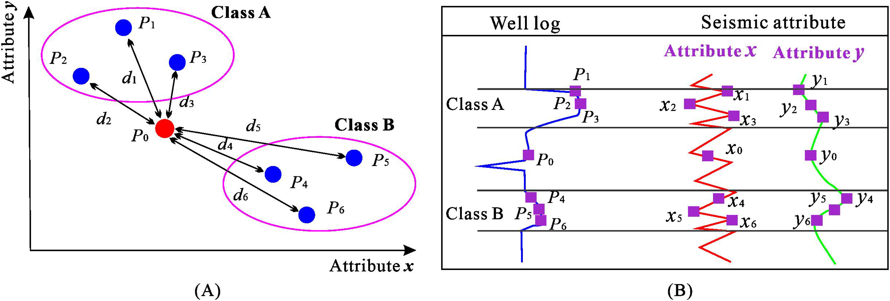
Correspondence between logging curves and seismic attributes of type A and type B lithologies.

Taking P1, P2, and P3 as training points, according to x₀ and y₀, the attribute value p0 can be predicted by the neural network:

P 0 = \frac{P 1 e^{- d_{1}^{2} / σ^{2}} + P 2 e^{- d_{2}^{2} / σ^{2}} + P 3 e^{- d_{3}^{2} / σ^{2}}}{e^{- d_{1}^{2} / σ^{2}} + e^{- d_{2}^{2} / σ^{2}} + e^{- d_{3}^{2} / σ^{2}}}

(4)

The σ is the rounding factor.

For both A and B lithologies:

g_{A} (P 0) = e^{- d_{4}^{2} / σ^{2}} + e^{- d_{5}^{2} / σ^{2}} + e^{- d_{6}^{2} / σ^{2}}

(5)

g_{B} (P 0) = e^{- d_{1}^{2} / σ^{2}} + e^{- d_{2}^{2} / σ^{2}} + e^{- d_{3}^{2} / σ^{2}}

(6)

The exponential weight function is adjusted by adjusting the value of σ to obtain different classifications. According to Bayes theorem, Prob is assigned to other lithological properties, namely:

pro b_{A} = \frac{g_{A} (P 0)}{g_{A} (P 0) + g_{B} (P 0)}

(7)

pro b_{B} = \frac{g_{B} (P 0)}{g_{A} (P 0) + g_{B} (P 0)}

(8)

The criterion is: if there is prob_A > prob_B at point P0, then point P0 belongs to class A; if prob_A < prob_B, then point P0 belongs to class B.

In the classification application, if there are three attributes and the convolution factor is 7, there are 3 × 7 = 21 sigmas to determine the relationship between known and unknown points.

There are two steps to determine the sigma value: ① First, assume that all sigmas have the same value. An optimal single sigma value is determined by experimenting with a series of sigma values and finding the Sigma with a minor validation error. ② The conjugate gradient iteration method determines the specific value of each Sigma.

The setting of the number of conjugate iterations is mainly to complete the second step. Using this single global Sigma as the starting point, the conjugate gradient algorithm is used to search for the sigma value related to each attribute that can minimize the verification error.

Results

Decompression correction

The sonic transit time curve retains the high-frequency variation details of the original sonic transit time curve after decompression correction with a long trend. It highlights the difference between reservoir and non-reservoir. Natural gamma can easily distinguish reservoirs from non-reservoirs. At the same time, the uncorrected DT is less effective for reservoir discrimination (Figure 10(a)). After the decompaction correction, the effect of acoustic transit on the distinction between reservoirs and non-reservoirs was significantly improved (Figure 10(b)).

Figure 10.

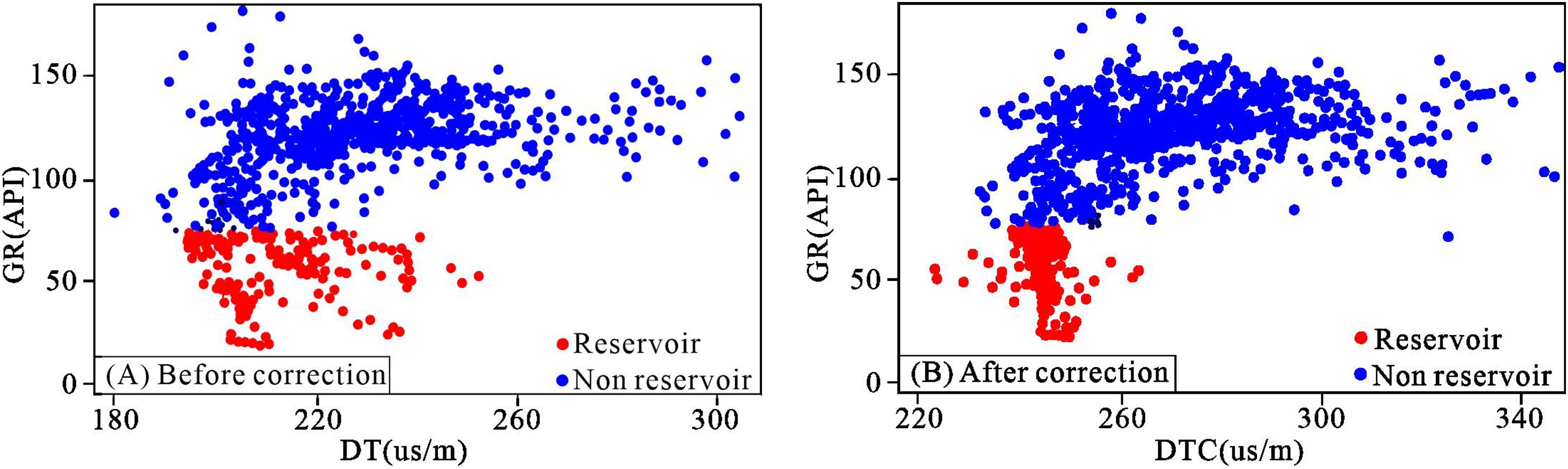
Comparison of acoustic time difference before and after decompaction correction in distinguishing reservoir and surrounding rock (DT: original sonic transit time, DTC: decompression corrected sonic transit time).

Seismic inversion after decompression correction

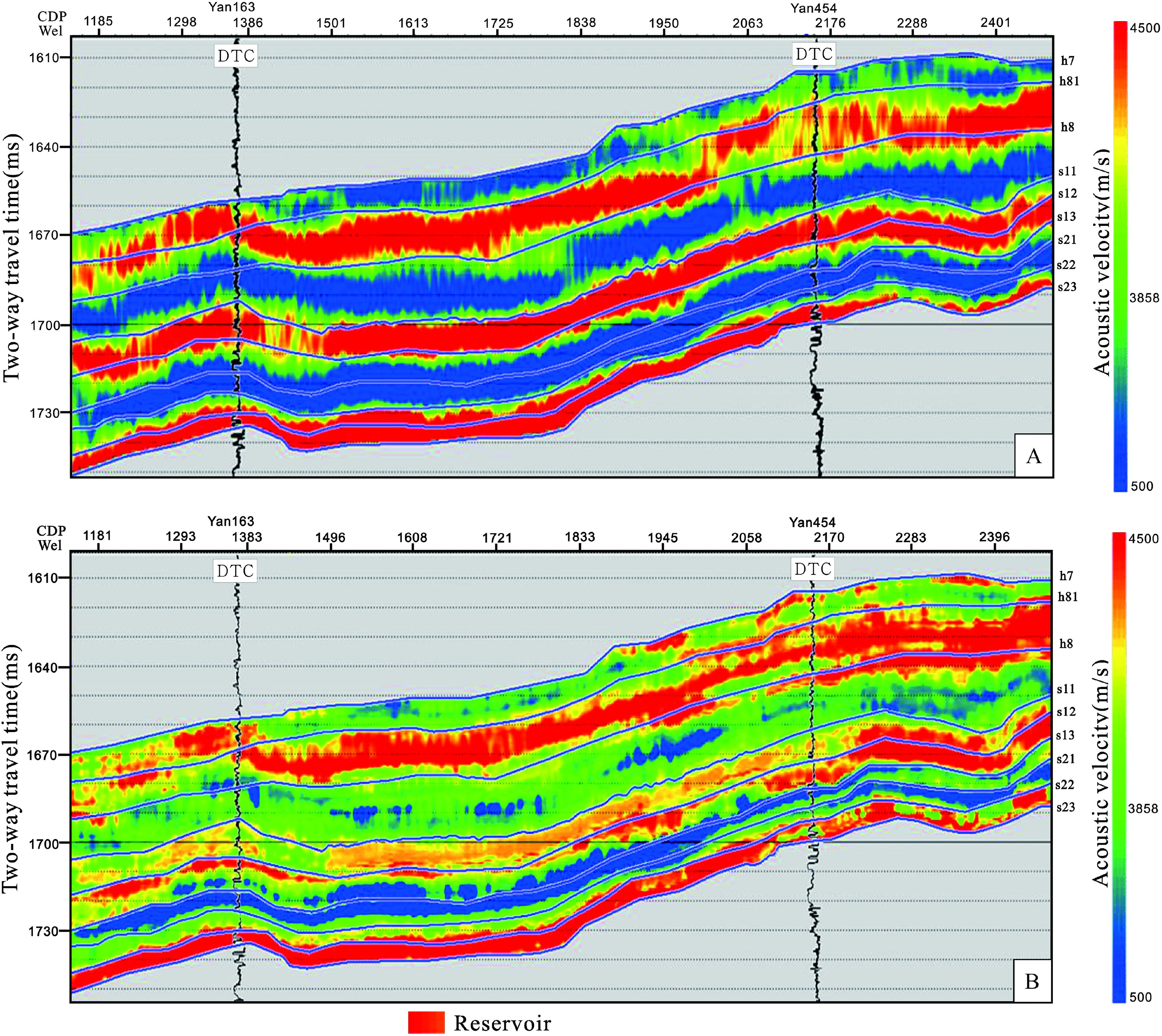
In order to illustrate the effect of decompaction correction on subsequent seismic inversion, logging-constrained inversion is performed by taking actual seismic lines as an example. The synthetic record calibration and model establishment were carried out using the two wells original and decompact corrected acoustic transit time curves. The corresponding velocity inversion profiles were formed after sparse pulse inversion and low-frequency trend loading (Figure 11). The overall variation trend of the formation after decompaction correction is more reasonable. The correlation between vertical velocity variation and lithology is higher. The resolution accuracy on the velocity inversion profile is significantly improved, and the lateral velocity band extends regularly. Because the overlapping area of the corresponding value of acoustic time difference between the reservoir and the surrounding rock decreases after the decompaction correction, the accuracy of identification of sandstone reservoir by acoustic time difference is improved.

Figure 11.

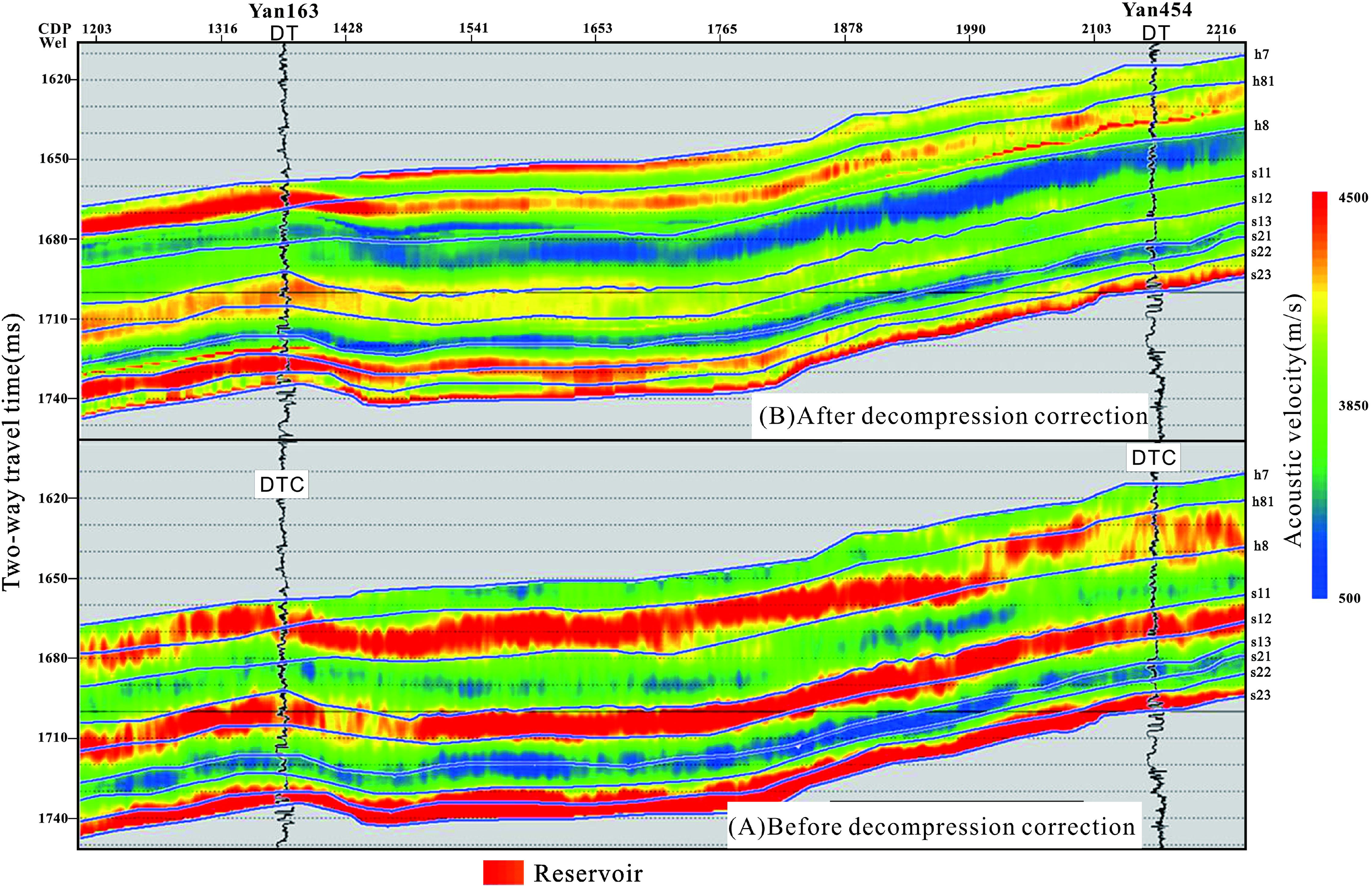
Comparison of logging constraint inversion effects before and after decompaction correction.

MPNN inversion

According to the seismic line test, the advantages of this research algorithm are verified by the actual processing and calculation of the seismic line. A conventional logging constraint inversion is first performed on the line to compare the advantages of multi-attribute probabilistic neural network inversion. The velocity profile of traditional impedance inversion is not high in vertical resolution. It cannot even resolve seismic waveforms (Figure 12A). The correlation between the inversion results of the well bypass and the well acoustic transit time curve is not high. This low correlation may be because conventional inversion needs to assume seismic wavelets; first, computational requirements limit wavelets, and only one average wavelet can be selected. Due to the insufficient vertical resolution, the velocity trend is extended too long in the horizontal direction. The correlation between the well-side channel and the well-acoustic transit time curve retrieved by the neural network reaches 92%. This study also compared multilayer feedforward neural networks (Lu and Jin, 1999; Dai et al., 2014; Kushwaha et al., 2020). The correlation between the well bypass and the well curve of the latter is 76%.

Figure 12.

Comparison of conventional wave impedance inversion and probabilistic neural network inversion.

Reservoir inversion and distribution prediction

After the test of the inversion method is completed, the established probability neural network is used to process the seismic data. That is, the acoustic velocity inversion is performed. According to the previous study, the value range of the decompression acoustic velocity response of the reservoir is 3900 m/s to 4400 m/s. According to the acoustic velocity profile obtained by neural network inversion, the reservoir samples are extracted and counted under the constraint of the top and bottom interface of the thin layer and then multiplied by the average velocity to obtain the reservoir thickness (Figure 13).

Figure 13.

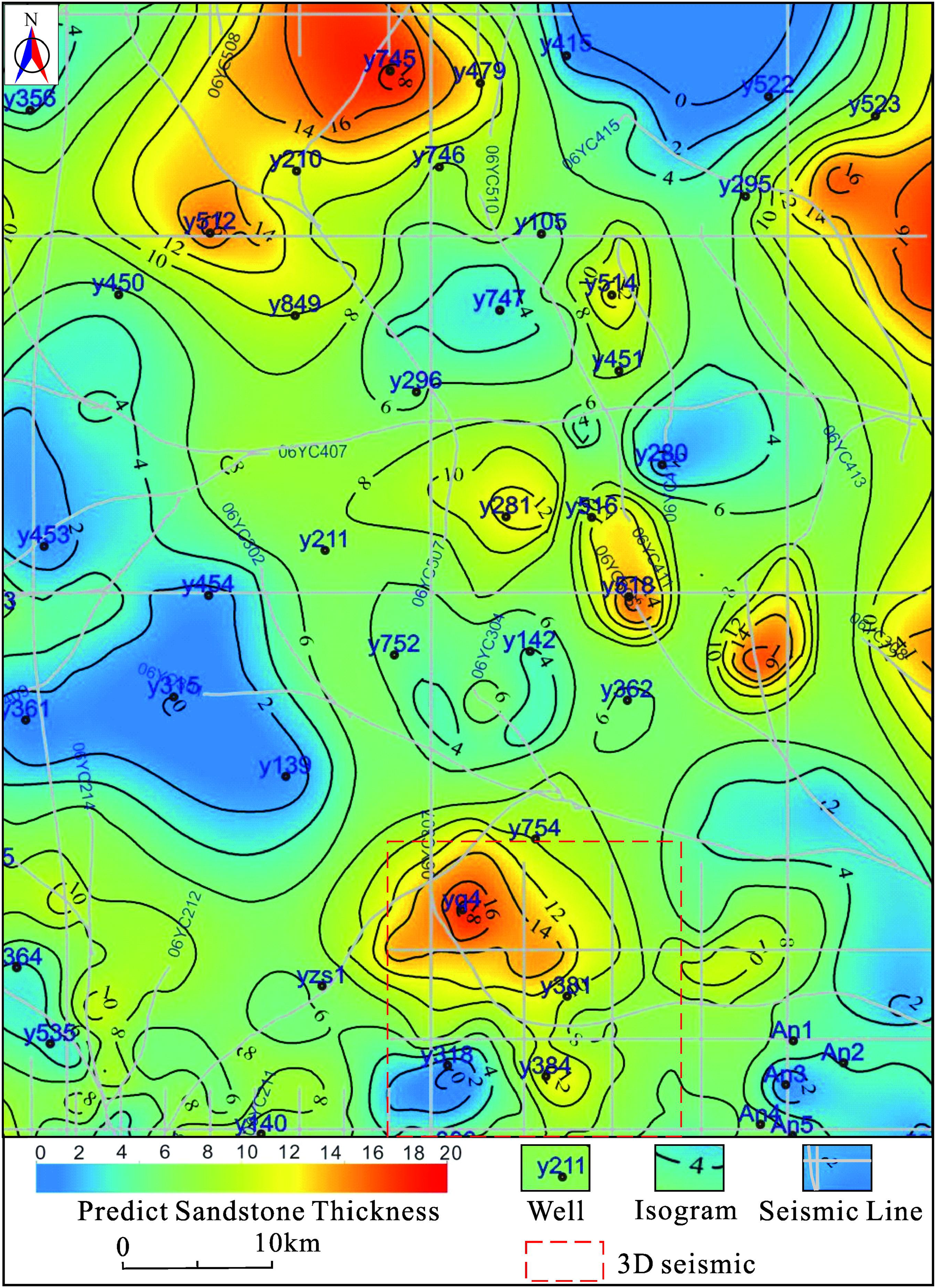
Prediction map of H₈¹ reservoir thickness in He 8 member of Yanchang gas field.

Discussions

Parameter experiment of MPNN

The geological relationship between seismic attribute combination and target logging attribute is not very clear, but the idea of this method is based on statistics. When the data volume is large enough, the stable nonlinear relationship between them can be obtained by using cross-validation technology, so that the high-precision logging attribute body can be obtained by inversion for geological interpretation (Herrera et al., 2006; Liu et al., 2016). There is a frequency difference between the target curve and the seismic attributes, a convolution factor must be introduced to resolve this difference. An optimal single sigma value is determined by experimenting with a series of values to find the Sigma with a minor validation error. Then the specific value of each Sigma is determined by the conjugate gradient iteration method. After selecting the nine best seismic attribute combinations, four experiments were carried out with different values of the convolution factor, the Sigma value of the rounding element and the number of iterations (Table 2).

Table 2.

Parameter test of probabilistic neural network.

Group	Sigma	Iterations	Convolution factor	Attribute number	Training time	Prediction error	Validation error
1	45	25	1	9	39	0.524	0.636
2	25	20	3	9	25	0.502	0.654
3	20	20	5	9	41	0.154	0.121
4	20	20	7	9	35	0.125	0.158

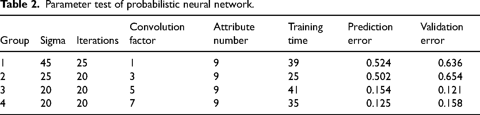
After increasing the Sigma and the number of iterations in experimental group 1 and experimental group 2, the prediction error and the verification error are close, indicating that the Sigma and the number of iterations have little effect on the increase or decrease of the error. Comparing several experimental groups, when the convolution factor is increased, the training error and the validation error gradually decrease, while the training time is different. This shows that the convolution factor has an important influence on accurate prediction results. The parameters of this neural network are determined by testing: the Sigma is 25, the number of iterations is 20, and the convolution factor is 7.

Characteristics of MPNN

The multi-attribute probabilistic neural network inversion utilizes the characteristics of the high vertical resolution of the logging curve, which reduces the inversion requirements for the quality of seismic data. The vertical resolution is higher, and more formation velocity changes can be seen. This change reveals the difference between sand and mudstone, and the prediction accuracy for thin sand bodies is higher (Figure 14).

Figure 14.

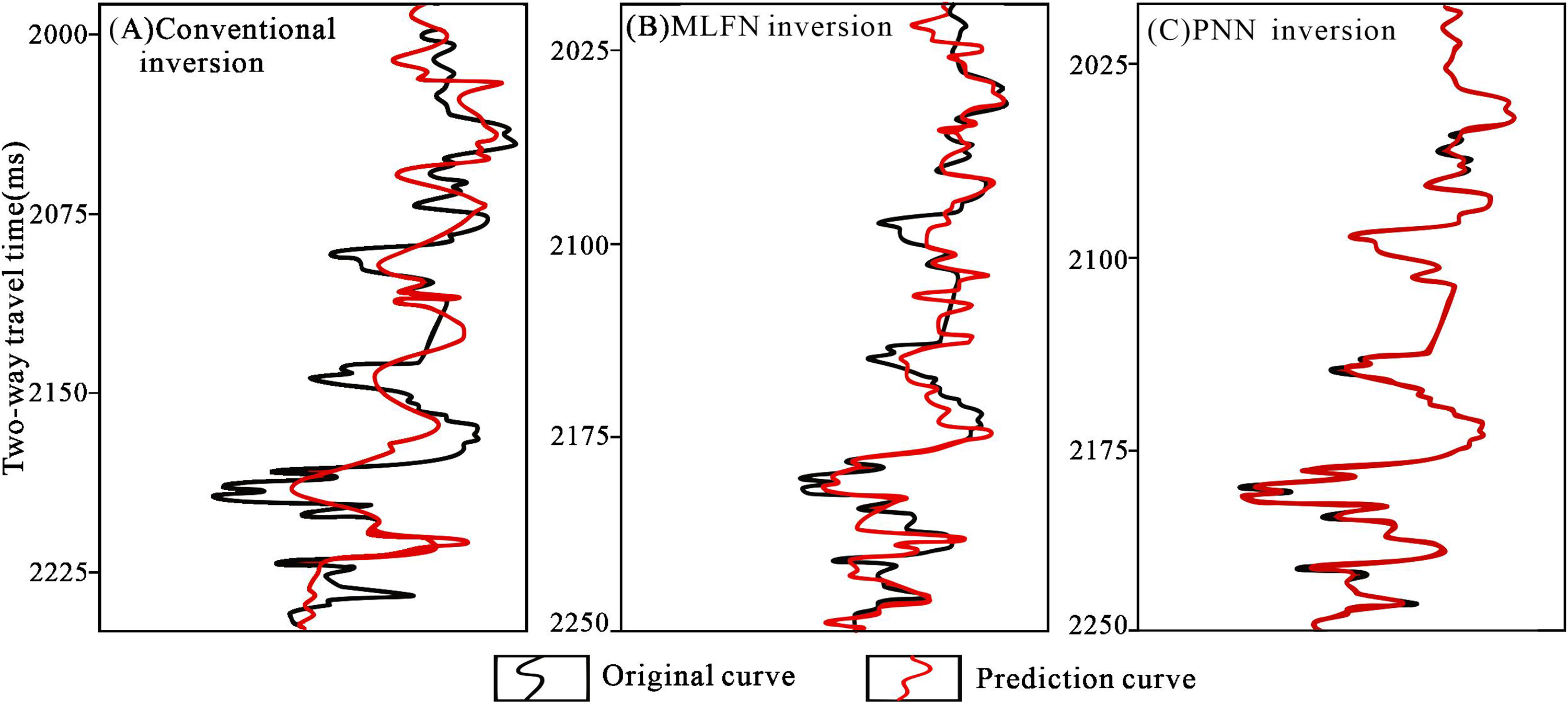
Comparison of three inversion velocities and logging sonic velocities (Well Y454).

From the results of multi-attribute neural network inversion, this method does not need to build a stratum model in advance and eliminates the dependence of traditional inversion on seismic wavelet. According to the logging curve, the probabilistic neural network fitting method is used and the seismic attributes and traditional inversion results are used as inputs to obtain the predicted results. In the calculation process, resampling technology is used to increase the number of vertical sampling points of seismic data, so that the vertical resolution of logging curves can be fully exploited, and the dependence of inversion on seismic data can be reduced, which almost reaches the same vertical resolution of logging curves in theory.

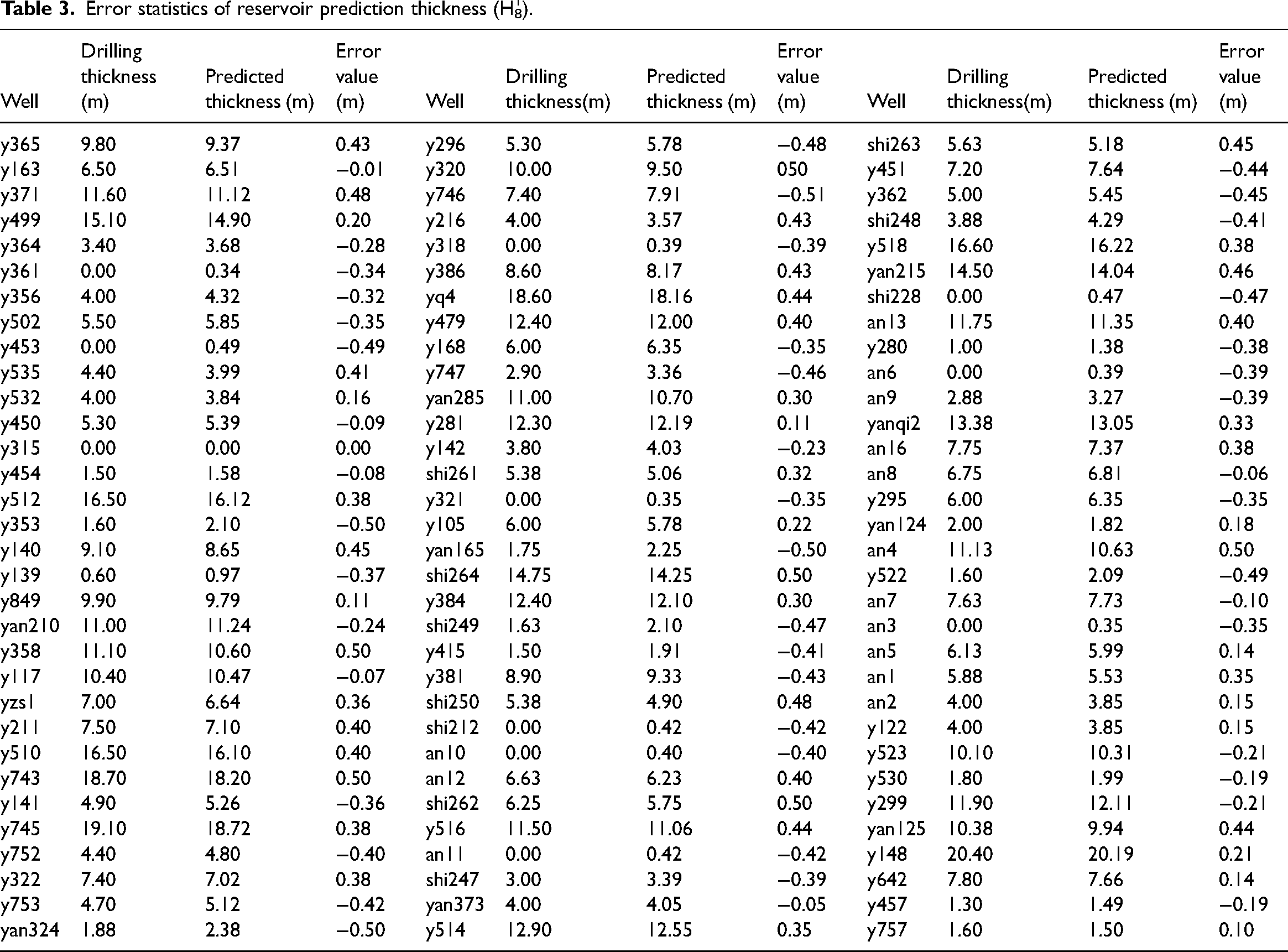
Evaluating the accuracy and effect of neural network inversion also needs to be cognisant of seismic data quality. In the seismic multi-attribute neural network inversion, the well-seismic attribute neural network model established using known well points needs to be extrapolated to the remaining seismic traces. Therefore, the quality of the seismic traces will inevitably affect the inversion accuracy of the neural network. Applying the above multi-attribute probabilistic neural network to predict the reservoir thickness of the H₈¹ in the Yanchang gas field shows that the method has high accuracy. Except for a few wells at the oilfield edge, most wells absolute error is less than 0.5 m (Table 3).

Table 3.

Error statistics of reservoir prediction thickness (H₈¹).

Well	Drilling thickness (m)	Predicted thickness (m)	Error value (m)	Well	Drilling thickness(m)	Predicted thickness (m)	Error value (m)	Well	Drilling thickness(m)	Predicted thickness (m)	Error value (m)
y365	9.80	9.37	0.43	y296	5.30	5.78	−0.48	shi263	5.63	5.18	0.45
y163	6.50	6.51	−0.01	y320	10.00	9.50	050	y451	7.20	7.64	−0.44
y371	11.60	11.12	0.48	y746	7.40	7.91	−0.51	y362	5.00	5.45	−0.45
y499	15.10	14.90	0.20	y216	4.00	3.57	0.43	shi248	3.88	4.29	−0.41
y364	3.40	3.68	−0.28	y318	0.00	0.39	−0.39	y518	16.60	16.22	0.38
y361	0.00	0.34	−0.34	y386	8.60	8.17	0.43	yan215	14.50	14.04	0.46
y356	4.00	4.32	−0.32	yq4	18.60	18.16	0.44	shi228	0.00	0.47	−0.47
y502	5.50	5.85	−0.35	y479	12.40	12.00	0.40	an13	11.75	11.35	0.40
y453	0.00	0.49	−0.49	y168	6.00	6.35	−0.35	y280	1.00	1.38	−0.38
y535	4.40	3.99	0.41	y747	2.90	3.36	−0.46	an6	0.00	0.39	−0.39
y532	4.00	3.84	0.16	yan285	11.00	10.70	0.30	an9	2.88	3.27	−0.39
y450	5.30	5.39	−0.09	y281	12.30	12.19	0.11	yanqi2	13.38	13.05	0.33
y315	0.00	0.00	0.00	y142	3.80	4.03	−0.23	an16	7.75	7.37	0.38
y454	1.50	1.58	−0.08	shi261	5.38	5.06	0.32	an8	6.75	6.81	−0.06
y512	16.50	16.12	0.38	y321	0.00	0.35	−0.35	y295	6.00	6.35	−0.35
y353	1.60	2.10	−0.50	y105	6.00	5.78	0.22	yan124	2.00	1.82	0.18
y140	9.10	8.65	0.45	yan165	1.75	2.25	−0.50	an4	11.13	10.63	0.50
y139	0.60	0.97	−0.37	shi264	14.75	14.25	0.50	y522	1.60	2.09	−0.49
y849	9.90	9.79	0.11	y384	12.40	12.10	0.30	an7	7.63	7.73	−0.10
yan210	11.00	11.24	−0.24	shi249	1.63	2.10	−0.47	an3	0.00	0.35	−0.35
y358	11.10	10.60	0.50	y415	1.50	1.91	−0.41	an5	6.13	5.99	0.14
y117	10.40	10.47	−0.07	y381	8.90	9.33	−0.43	an1	5.88	5.53	0.35
yzs1	7.00	6.64	0.36	shi250	5.38	4.90	0.48	an2	4.00	3.85	0.15
y211	7.50	7.10	0.40	shi212	0.00	0.42	−0.42	y122	4.00	3.85	0.15
y510	16.50	16.10	0.40	an10	0.00	0.40	−0.40	y523	10.10	10.31	−0.21
y743	18.70	18.20	0.50	an12	6.63	6.23	0.40	y530	1.80	1.99	−0.19
y141	4.90	5.26	−0.36	shi262	6.25	5.75	0.50	y299	11.90	12.11	−0.21
y745	19.10	18.72	0.38	y516	11.50	11.06	0.44	yan125	10.38	9.94	0.44
y752	4.40	4.80	−0.40	an11	0.00	0.42	−0.42	y148	20.40	20.19	0.21
y322	7.40	7.02	0.38	shi247	3.00	3.39	−0.39	y642	7.80	7.66	0.14
y753	4.70	5.12	−0.42	yan373	4.00	4.05	−0.05	y457	1.30	1.49	−0.19
yan324	1.88	2.38	−0.50	y514	12.90	12.55	0.35	y757	1.60	1.50	0.10

Applicability and limitation of MPNN

A probabilistic neural network has certain requirements in terms of the number of wells, and the selection of attribute types and numbers should have a good correlation with the wave impedance value, which needs to be fully considered in the inversion process (Xie et al., 2015). For complex structural areas, such as small fault-block oil and gas reservoirs, pre-stack gathers used for analysis are usually low in signal-to-noise ratio, and the effect of this method may be unsatisfactory. Therefore, the neural network inversion technology based on pre-stack seismic attributes and pre-stack inversion can only be applied to areas with good seismic data quality, especially in relatively simple structures but complex lithology. Only under the premise of targeted amplitude-preserving processing of seismic data can better prediction and evaluation results be achieved. However, this method is mainly based on analyzing rock physical properties and lacks the understanding of subjective geological concepts. The accuracy and rationality of reservoir prediction will be higher if artificial subjective geological factors such as sedimentary facies are added (Ashraf et al., 2022; Anees et al., 2022a, 2022b).

Conclusion

Taking Carboniferous and Permian in the southeast of Ordos Basin as an example, this study expounds the multi-attribute probabilistic neural network seismic reservoir prediction method based on mudstone compaction correction. In the inversion velocity profile after decompaction correction, the overall variation trend of the formation is more reasonable, and the correlation between the vertical velocity variation trend and lithology is higher. After sonic decompaction correction, the resolution accuracy on the velocity inversion profile is significantly improved, the lateral velocity strips extend regularly, and the degree of agreement with the well is also enhanced to a certain extent.

Multi-attribute probabilistic neural network seismic inversion method is a typical nonlinear algorithm. It uses the stepwise regression method to sort the prediction effects of attributes, determines the convolution factor and the types and numbers of seismic attributes involved in the operation with the help of the idea of cross-validation, and establishes the relationship between various seismic attributes and logging values through linear regression analysis and probabilistic neural network method, so as to make the prediction results of probabilistic neural network reach the best.

Compared with traditional inversion methods such as sparse pulse inversion, probabilistic neural network inversion has better resolution and can better approximate the real value. This method can effectively identify sandstone and mudstone with similar physical properties, and effectively improve the identification accuracy of reservoirs. Probabilistic neural network has certain requirements on the number of wells, and the selection of attribute types and numbers should have a good correlation with the wave impedance value.

Footnotes

Acknowledgements

Financial supports of this study by the National Natural Science Foundation (No. 41372118, 41002043) are acknowledged. Sincere gratitude should go to professor Kenneth A. Eriksson who helped me in the revision of my paper. We are grateful to editor in chief professor Yuzhuang Sun and reviewers for their effort reviewing our paper and their positive suggestion.

Declaration of conflicting interests

The author(s) declared no potential conflicts of interest with respect to the research, authorship, and/or publication of this article.

Funding

The author(s) disclosed receipt of the following financial support for the research, authorship, and/or publication of this article: This work was supported by the National Natural Science Foundation of China, (grant numbers 41372118, 41002043).

ORCID iD

Feng Guo

References

Abdideh

Dastyaft

(2022) Stress field analysis and its effect on selection of optimal well trajectory in directional drilling (case study: Southwest of Iran). Journal of Petroleum Exploration and Production Technology 12(3): 835–849.

Anees

Zhang

Umar

, et al. (2021) Identification of favorable zones of gas accumulation via fault distribution and sedimentary facies: Insights from Hangjinqi area, Northern Ordos. Basin.Frontiers in Earth Science 9: 1–16.

Anees

Zhang

Umar

, et al. (2022a) Sand-ratio distribution in an unconventional tight sandstone reservoir of Hangjinqi area, Ordos Basin: Acoustic impedance inversion-based reservoir quality prediction. Frontiers in Earth Science 10: 1–14.

Anees

Zhang

Umar

, et al. (2022b) Sedimentary facies controls for reservoir quality prediction of lower Shihezi member-1 of the Hangjinqi area, Ordos Basin. Minerals 12: 1–19.

Dai

Zhang

Jiang

, et al. (2014) Research on nonlinear analysis of geological data based on multilayer feedforward neural network SPDS algorithm. Communist China. Science Abstracts 36(08): 1528–1532.

Daniel

(2001) Use of multiattribute transforms to predict log propertied from seismic data. Geophysics 66(1): 220–236.

Ding

Yin

, et al. (2018) Prediction method of seismic reflection mode based on probabilistic neural network with geological information constraints. China Offshore Oil and Gas 30(01): 127–131.

Song

Sun

((2010) Seismic reservoir interpretation technology. Beijing: Petroleum Industry Press.

Ashraf

Zhua

Yasin

, et al. (2019) Classification of reservoir facies using well log and 3D seismic attributes for prospect evaluation and field development: A case study of Sawan gas field, Pakistan. Journal of Petroleum Science & Engineering 175, 338–351.

10.

Emilson

Alexandre

(2010) 3D Porosity prediction from seismic inversion and neural networks. Computers & Geosciences 37(8): 1174–1180.

11.

Feng

(2020) Estimation of reservoir porosity based on seismic inversion results using deep learning methods. Journal of Natural Gas Science and Engineering 77: 1–9.

12.

Gong

, et al. (2009) Reservoir prediction method based on seismic attributes-taking the second member of Shahejie formation in Yong ‘an area as an example. Marine Geology & Quaternary Geology 29(06): 95–102.

13.

Guo

Luo

, et al. (2021) Seismic rock physics inversion with varying pore aspect ratio in tight sandstone reservoirs. Journal of Petroleum Science & Engineering 207: 1–11.

14.

Hampson

Schuelke

Quirein

(2001) Use of multiattribute transforms to predict log properties from seismic data. Geophysics 66: 220–236.

15.

Herrera

Russel

Flores

(2006) Interpreter's corner: Neural networks in reservoir characterization. The Leading Edge 25(4): 402–411.

16.

Kushwaha

Maurya

Rai

, et al. (2020) Porosity prediction from offshore seismic data of F3 block, The Netherlands using multi-layer feed-forward neural network. Current Science 119(10): 1652–1662.

17.

Lai

Cao

Zhang

(2020) Decompaction correction of acoustic transit time difference in long trend. Oil Geophysical Prospecting 55(05): 1102–1109.

18.

Lee

Shin

Son

, et al. (2022) Zero-offset data estimation using CNN for applying 1D full waveform inversion. Journal of Geophysics 19: 39–50.

19.

, et al. (2000) A new decompaction correction method. Experimental Petroleum Geology 22(2): 110–114.

20.

Liu

Zhao

Sun

(2009) Tectonic background of Ordos Basin and its controlling role for basin evolution and energy mineral deposits. Energy Exploration and Exploitation 27(1): 15–27.

21.

Liu

, et al. (2014) The relationship between the mechanical compaction and the densification process of sandstones and the affect degree of compaction to the densifying of Yanchang formation, Ordos Basin. International Geology Review 60(3): 655–665.

22.

Liu

Pei

(2016) Inversion and prediction of coal seam roof lithology by multi-attribute neural network. Coal Geology & Exploration 44(01): 103–106. +111.

23.

Jin

(1999) Lithology identification method based on feedforward neural network. Oil & Gas Geology 20(01): 84–86, 95.

24.

Fang

Wang

, et al. (2004) Prediction of reservoir distribution by seismic multi-attribute transformation. Petroleum Geology and Engineering 18(4): 16–20.

25.

Masters

(1994) Signal and Image Processing with Neural Networks. New York: John Wiley & Sons Incorporation, 1–200.

26.

Maurya

Singh

(2018) Application of LP and ML sparse spike inversion with probabilistic neural network to classify reservoir facies distribution - A case study from the blackfoot field, Canada. Journal of Geological Science 2018: 159.

27.

McCormack

(1991) Neural computing in geophysics. Leading Edge 10(1): 11–15.

28.

Meldahl

Heggland

Bril

, et al. (1999) The chimney cube,an example of semi-automated detection of seismic objects by directive attributes and neural networks: Part I; methodology. SEG Technical Program Expanded Abstracts 18(1): 931–934.

29.

Nikravesh

Aminzadeh

(2001) Mining and fusion of petroleum data with fuzzy logic and neural network agents. Journal of Petroleum Science & Engineering 29: 221–238.

30.

Perrier

Quilbier

(1974) Thickness changes in sedimentary layers during compaction history. AAPG Bulletin 58: 507–520.

31.

Yang

(2001) A discussion about the method of decompaction correction. Petroleum Geology & Experiment 23(3): 351–356.

32.

Roth

Tarantola

(1994) Neural networks and inversion of seismic data. Journal of Geophysical Research: Solid Earth 99: 6753–6768.

33.

Sircar

Yadav

Rayavarapu

, et al. (2021) Application of machine learning and artificial intelligence in oil and gas industry. Petroleum Research 6(4): 379–391.

34.

Soleimani

(2013) Simulation of oil and gas exploration based on conceptual decision model-taking dezver bay in southwest Iran as an example. Petroleum Exploration and Development 40(04): 443–447.

35.

Sun

Liu

Lin

, et al. (2009) Geochemical evidences of natural gas migration and releasing in the Ordos Basin, China. Energy Exploration and Exploitation 27(1): 1–13.

36.

Trappe

Hellmich

(1995) Using neural networks to predict porosity thickness from 3D seismic. First Break 18: 377–384.

37.

Triveni

Rima

(2019) Estimation of petrophysical parameters using seismic inversion and neural network modeling in upper assam basin, India. Geoscience Frontiers 10(3): 1113–1124.

38.

Walls

Taner

Taylor

, et al. (2002) Seismic reservoir characterization of a U.S. Midcontinent fluvial system using rock physics, poststack seismic attributes, and neural networks. Leading Edge 21: 428–436.

39.

Withers

(1992) The value of reservoir geophysics. Leading Edge 11(3): 35–39.

40.

(1989) Method of formation compaction correction using logging and seismic data. Oil Geophysical Prospecting 1 (01): 68–79.

41.

Xie

Zheng

, et al. (2015) Application of seismic multi-attribute probabilistic neural network (PNN) inversion based on cross-validation in identifying igneous rocks in rewap area. China Mining Magazine 24(02): 154–158.

42.

Yang

Qiao

(2021) Research on reconstruction method of pseudo acoustic transit log based on multiple regression mode. Uranium Geology 37(03): 500–505.

43.

Yang

(2003) Method of delaminated decompaction correction. Petroleum Geology & Experiment 25(2): 206–210.

44.

Yazmyradova

Hassan

Anis

, et al. (2021) Reservoir characterisation of high-pressure, high-temperature zone of malay basin using seismic inversion and artificial neural network approach. Applied Sciences 11(1): 1–27.

45.

Zhang

Lei

Chen

, et al. (2015) Study on debris flow prediction based on Bayesian classifier of rainfall. Journal of Chengdu University(Natural Science Edition) 34(01): 94–96.

46.

Zhang

Dong

Shen

, et al. (2005) Application of log rebuilding technique in constraining inversion. Petroleum Exploration and Development 32(3): 70–72.

47.

Zhu

Cui

Chen

, et al. (2021) Sedimentary system and reservoir petrological characteristics of shallow water delta-taking shan 1-he 8 member in western Ordos Basin as an example. Acta Sedimentary Sinica 39(01): 126–139.

Multi-attribute Probabilistic Neural Network Reservoir Prediction Based on Mudstone Acoustic Time Difference Decompaction Correction

Abstract

Keywords

Introduction

Geological setting

Data and methods

Acoustic wavelength trend decompaction correction

Multi-attribute probabilistic neural network modeling (MPNN)

Results

Decompression correction

Seismic inversion after decompression correction

MPNN inversion

Reservoir inversion and distribution prediction

Discussions

Parameter experiment of MPNN

Characteristics of MPNN

Applicability and limitation of MPNN

Conclusion

Footnotes

Acknowledgements

Declaration of conflicting interests

Funding

ORCID iD

References