Sage Journals: Discover world-class research

Abstract

Conventional fracture closure models typically assume homogeneous formation. This assumption renders complex fracture closure pressure analysis during shut-in insufficient at present. In this paper, we use a cohesive zone method (CZM)-based finite element model to obtain the fracture closure pressure and minimum horizontal principal stress of the major fracture and the branch fracture based on pressure fall-off analysis. Key factors including leak-off rate, injection time, and stress anisotropy are discussed in detail. A quantitative relationship between fracture closure pressure and these factors is plotted to reduce or eliminate the errors caused by conventional fracture injection diagnostic models. The results show that leak-off rate, injection time, and stress anisotropy have a significant effect on the fracture closure process. Fracture closure in naturally fractured formations is a slow process, and the early closure pressure represents the closure of the branch fracture, which is much higher than the minimum horizontal stress. This investigation provides new insight into how to estimate the in-situ stress in naturally fractured reservoirs.

Keywords

Fracture closure complex fracture network shut-in decline hydraulic fracturing stress measurement

Introduction

Hydraulic fracturing is a well stimulation technology that is effective in increasing hydrocarbon production in unconventional reservoirs such as shale gas, coal-bed methane, and tight sandstone (Montgomery and Smith, 2010; Dahi Taleghani et al., 2020; Wang et al., 2020b). A large volume of viscous fluid is continuously injected into such a formation to promote hydraulic fracture propagation, which occurs at a depth of several thousand metres and accordingly cannot be directly observed. The hydraulic fracturing process is very complex (Nolte, 1986; van Dam et al., 2000; Smith and Montgomery, 2015). However, the pressure data recorded at the time of an injection via a diagnostic fracture injection test (DFIT) can provide a wealth of information on fracture geometry, fluid leak-off characteristics, and fracture closure time (Nolte, 1986, 1991; Mayerhofer et al., 1995; Plahn et al., 1997). Among DFITs, fracture pressure decline analysis is a common method of determining the fracture closure pressure and closure time due to the elimination of wellbore friction after shut-in (de Pater et al., 1996; Kholy et al., 2019). Thus, fracture closure analysis has been one of the trending topics in research on hydraulic fracturing over the past decades.

A laboratory experiment was designed to investigate hydraulic fracture closure behaviour in different materials, including cement, plaster, soft plaster, and diatomite (van Dam et al., 2000). The results showed that the radius changes of penny-type fractures after shut-in significantly influence fluid leak-off characteristics, mechanical behaviour, and fracture closure pressure. The closure time increases as the fractured radius decreases in size, while the calculated leak-off coefficient is overestimated when the fractured radius increases in size.

Over the last few decades, different fracture closure models have been developed to determine key parameters such as closure pressure, formation permeability, leak-off coefficient, and fluid efficiency. These models include the square root plot, log-log plot, G-function plot, and empirical equation (Nolte, 1986, 1991; Barree et al., 2007; Belyadi et al., 2019; Kholy et al., 2019). The square root plot suggests that closure pressure occurs at the inflection point on the second derivative of pressure (Belyadi et al., 2019). The straight line between the origin and the inflection point deviates from the second derivative curve. The log-log plot is employed to determine fracture closure and various flow regimes such as the linear flow regime, bilinear flow regime, and pseudoradial flow regime (Mayerhofer et al., 1995; Barree et al., 2007). Closure occurs at the point where the slope of the second derivative curve changes from positive to negative. G-function derivative analysis requires a plot that includes the bottom-hole pressure, the pressure derivative (dP/dG), and the superimposed pressure derivative (GdP/dG). The characteristic curved shape of the pressure derivative and the superposition pressure derivative is used to identify the leak-off behaviour, of which there are four common types, i.e, normal leak-off behaviour, pressure-dependent leak-off from opened natural fractures, fracture-height recession during shut-in, and fracture-tip extension (McLellan and Janz, 1991; Barree and Mukherjee, 1996; Craig et al., 2000; Chipperfield, 2006; Cai and Dahi Taleghani, 2021). Plahn et al. (1997) proposed a numerical model of the fracture pump-in and flow-back test, which gives a better estimate of fracture closure pressure than the aforementioned conventional methods. Based on the signal processing approach, Eltaleb et al. (2021) proposed a novel methodology for DFIT analysis in geothermal reservoirs, which is independent of rock mechnical properties and fracture geometry. Wang et al. (2021b) anaylzed the characteristic of pressure decline in fractured horizontal wells, and build up a new model which can quantitatively estimate closure stress and average pore pressure. This model can also infer the uniformity of proppant distribution in the hydraulic fractures. Carpenter (2021) pointed out that a slow increase in the dP/dG plot indicates that long-time fracture closure is caused by early near-wellbore fracture closure.

However, it is not practical to use the aforementioned fall-off analysis methods to determine fracture closure pressure in tight formations because the closure time is very long (Barree et al., 2014). Kholy et al. (2019) developed an empirical equation to predict hydro-fracture closure pressure based on the instantaneous shut-in pressure (ISIP) using subsurface solids-injection data. The newly proposed method can be used to obtain the fracture closure pressure with a relative error of less than 3% compared to the closure pressure measured in the oilfield. Noting that a hydraulic fracture retains a limited width after asperities come into contact, McClure et al. (2016) proposed a fracture compliance method that picks up the fracture closure pressure from DFITs. Afterwards, the proppant transport with gravitational settling and fracture closure are integrated into a three-dimensional (3D) hydraulic fracture simulator (Shiozawa and McClure, 2016). A new constitutive equation is introduced into the 3D simulator and can seamlessly describe the fracture closure process during shut-in. This model includes the nonlinear joint closure law denoting fracture compliance and fracture surface roughness, as well as the effect of proppant accumulation in the hydro-fractures. He et al. (2017) considered the different gas-rate production values of fractures and developed a semi-analytical method to diagnose the locations of underperforming hydro-fractures through pressure-transient analysis in tight gas reservoirs. This method was derived from the Green function and was verified by comparison using the commercial software KAPPA Ecrin. Using post-closure pulse testing, Upchurch (2003) developed a method to determine the fracture closure pressure in soft formations. This method was likewise verified with several field examples. No reduction in the accuracy of the leak-off coefficient when compared to the recorded pressure data was found. Cai and Dahi Taleghani (2021) numerically investigated the inititation and closure behaviour of an axial fracture during DFIT, and the results show that the closure time of the axial fracture from fracture compliance based DFIT analysis is earlier than that of the transverse fracture. They recommend that the combined method of the G × dP/dG plot and the dP/dG plot is helpful for DFIT interpretation.

Taken together, the current fracture closure models do not consider the long closure process of complex fracture networks including branch fractures. Furthermore, the effect of geomechanical behaviour on fracture closure is not fully integrated into the calculations of the fluid flow and leak-off in the current fracture closure models. Which fracture closes first after shut-in: the main hydraulic fracture or the branching hydraulic fracture? Errors may occur when field technicians employ a conventional closure model to identify the closure pressure or minimum horizontal principal stress (σ_h) in tight formations. According to Barree et al. (2014), such poor or nonexistent results stem from either problematic data acquisition or the incorrect analysis of the acquired data.

The goal of this paper is to numerically investigate complex fracture closure pressure analysis during shut-in. We employ a cohesive zone method (CZM)-based finite element model to identify the fracture closure pressure and minimum horizontal principal stress of major and branch fractures from pressure fall-off analysis. Key factors including leak-off rate, injection time, and stress anisotropy are discussed in detail. A quantitative relationship between fracture closure pressure and these factors is plotted to reduce or eliminate the errors caused by conventional fracture injection diagnostic models. This investigation provides new insight into how to estimate the in-situ stress in naturally fractured reservoirs.

The paper is organized as follows: The “Method and Theory” section presents the governing equations of hydraulic fracturing problems, including the stress equilibrium equation for rock deformation and the lubrication equation for fluid flow in hydraulic fractures. The “Numerical Simulation” section discusses the effects of key factors including leak-off coefficient, injection time, and stress anisotropy on the fracture closure pressure and in-situ stress estimation. The quantitative relationship between fracture closure pressure and these factors is also presented. The main conclusions of this study are summarized in the last section.

Method and theory

We consider the hydraulic fracture closure process to be a two-dimensional (2D) coupled stress-seepage field problem in porous media. This problem consists of a rock matrix that includes predefined zero-thickness cohesive elements representing the hydraulic fracture propagation paths. CZM is utilized to simulate the damage initiation and evolution of hydraulic fracturing problems (Barenblatt, 1962; Wang et al., 2018b; Wang et al., 2020a).

The coupled problem consists of rock deformation and fluid flow in the rock matrix and fracture networks. Fluid exchange exists between the porous rock matrix and fractures. The pore space of the rock matrix is considered fully saturated. We assume that only a single-phase flow exists in the rock matrix, as this type of flow usually dominates the early flow-back process. We assume the fluid flow in the rock matrix obeys Darcy's flow. According to the theory of linear poroelasticity (Biot, 1941), the governing equation for the rock matrix is expressed as

σ_{i j} - σ_{i j}^{0} = \frac{E}{1 + ν} (ε_{i j} + \frac{ν}{1 - 2 ν} ε_{k k} δ_{i j}) - α (p - p_{0}) δ_{i j}

(1)

where σ_ij are the geo-stress components; σ⁰ _ij are the initial geo-stress components; E is the elastic modulus of rock; ν is Poisson's ratio; α is the Boit constant; ε_ij are the strain components; p is the pore pressure; and p₀ is the initial pore pressure. It is worth noting that we use initial stress to obtain a more efficient convergence of our numerical model.

According to the principle of mass balance, the fluid flow in fractures is expressed as

\frac{\partial w_{f}}{\partial t} + \frac{\partial (w_{f} v_{t})}{\partial x} + v_{n} = 0

(2)

where w_f is fracture width; t is injection time; x is fracture location; v_n is the leak-off velocity normal to fracture surface (Carter, 1957); and v_t is the fluid velocity along the fracture.

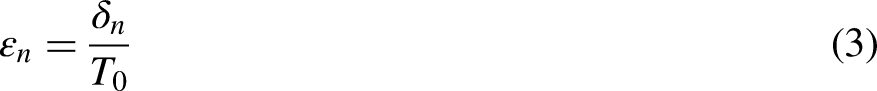
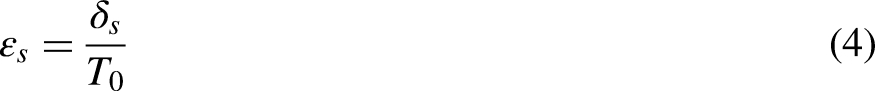
The nominal strains are expressed as

ε_{n} = \frac{δ_{n}}{T_{0}}

(3)

ε_{s} = \frac{δ_{s}}{T_{0}}

(4)

where δ_n and δ_s are the normal and shear separation, respectively; ε_n and ε_s are the nominal strain components in the normal and shear directions, respectively; and T₀ is the initial thickness of the cohesive elements. According to traction-separation law (TSL), the constitutive equation of the cohesive elements is expressed as

t = {\begin{matrix} t_{n} \\ t_{s} \end{matrix}} = [\begin{matrix} E_{n n} & E_{n s} \\ E_{n s} & E_{s s} \end{matrix}] {\begin{matrix} ε_{n} \\ ε_{s} \end{matrix}}

(5)

where t_n and t_s are the two components of nominal stress traction vector t in the normal and shear directions, respectively; and E_nn, E_ns, and E_ss are the components of elastic constitutive matrix E.

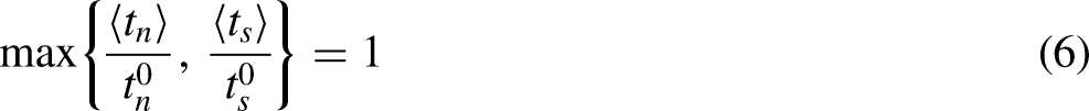
The maximum nominal stress criterion is utilized to represent damage initiation. The criterion is expressed as

max {\frac{⟨ t_{n} ⟩}{t_{n}^{0}}, \frac{⟨ t_{s} ⟩}{t_{s}^{0}}} = 1

(6)

where t_n⁰ and t_s⁰ are the peak values of the nominal stress traction vector in the normal and shear directions, respectively. The bilinear TSL, which is suitable for sedimentary rocks in practical applications (Dahi Taleghani et al., 2013), is used to model the fracture zone process in this study. The traction linearly increases with the increase in separation before damage initiation. The cohesive elements are damaged once the traction reaches its peak value. After that, the traction linearly decreases with the increase in separation. When the traction reaches zero, complete damage occurs in the cohesive elements.

As shown in Figure 1, a 2D plane strain model is used to represent the coupled stress-seepage field problem in ABAQUS. The size of the square domain is 200 m × 200 m. The symmetric finite element model is used to reduce the computation cost. The injection point is located at the centre of the left edge. Two groups of cohesive elements (i.e. a hydraulic fracture and a natural fracture, denoted by the red lines in Figure 1) are inserted into the unstructured meshes to represent the possible fracture propagation and closure paths during flow-back. The approach angle between the hydraulic fracture and the natural fracture is denoted as β. Although we focus on flow-back in this study, we include the injection stage in our numerical simulations to provide a realistic fracture pattern for an initial condition of the flow-back model.

Figure 1.

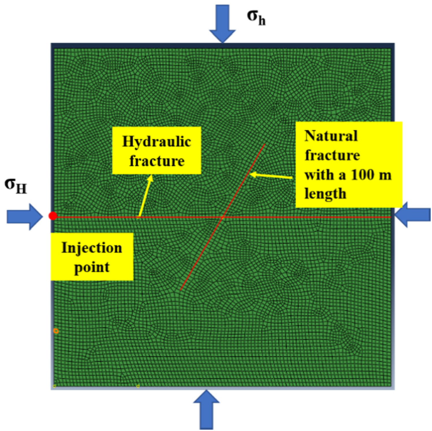
2D Plane strain model in ABAQUS.

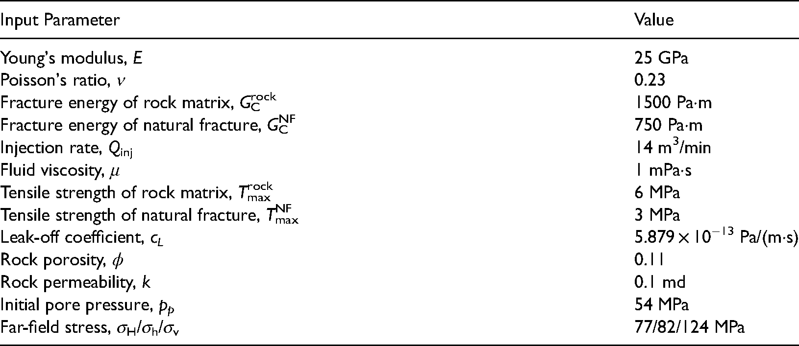
We conduct a single planar fracture propagation as the initial simulation to provide an accurate initial condition during flow-back for verification and validation ends. The input parameters for the flow-back simulation model are listed in Table 1, which are from the MaHu tight oil reservoir in Xinjiang Autonomous Region, China. In this planar fracture model, the minimum horizontal stress σ_h, the maximum horizontal stress σ_H, and the overburden stress σ_v are equal to 77 MPa, 82 MPa, and 124 MPa, respectively, and pore pressure is equal to 54 MPa. The rock matrix is considered to be a linear elastic medium in which E = 25 GPa and ν = 0.23. The CZM parameters of E_nn and K_n are set to 25 GPa and 87.5 GPa, respectively. A linear elastic TSL is used to represent the damage evolution during hydraulic fracturing. Complete cohesive element failure occurs when the fracture energy satisfies the Benzeggagh-Kenane fracture criterion (Benzeggagh and Kenane, 1996). The calculated initial fracture width and the net pressure within the hydro-fracture before the simulation of flow-back presents a non-uniform distribution. Therefore, the analytical step of modelling fracture propagation in ABAQUS plays a very important role in simulating fracture closure during flow-back.

Table 1.

Input parameters for the flow-back simulation model.

Input Parameter	Value
Young's modulus, E	25 GPa
Poisson's ratio, ν	0.23
Fracture energy of rock matrix, G_C^rock	1500 Pa·m
Fracture energy of natural fracture, G_C^NF	750 Pa·m
Injection rate, Q_inj	14 m³/min
Fluid viscosity, μ	1 mPa·s
Tensile strength of rock matrix, T_max^rock	6 MPa
Tensile strength of natural fracture, T_max^NF	3 MPa
Leak-off coefficient, c_L	5.879 × 10⁻¹³ Pa/(m·s)
Rock porosity, $ϕ$	0.11
Rock permeability, k	0.1 md
Initial pore pressure, p_p	54 MPa
Far-field stress, σ_H/σ_h/σ_v	77/82/124 MPa

Numerical simulation

In this section, we use a CZM-based finite element model to simulate the major and branch fracture closure processes. Key factors including approach angle, injection time, leak-off rate, and horizontal stress difference are analysed in detail. As shown in Figure 1, the major fracture is a part of the hydraulic fracture in the horizontal direction, and the branch fracture is a part of the natural fracture in the inclined direction.

Model verification

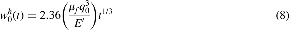
To verify the CZM-based finite element model, the numerical solutions are compared to the analytical solutions. The analytical solutions are derived from the famous KGD hydraulic fracturing model (Zheltov, 1955; Geertsma and De Klerk, 1969). The fracture length $L_{f r a c} (t)$ and fracture width at the injection point $w_{h}^{0} (t)$ are respectively expressed as in Eqs. (7) and (8).

L_{f r a c} (t) = 1.078 {(\frac{E^{'} q_{0}^{3}}{μ_{f}})}^{1 / 6} t^{2 / 3}

(7)

w_{0}^{h} (t) = 2.36 (\frac{μ_{f} q_{0}^{3}}{E^{'}}) t^{1 / 3}

(8)

where t is the injection rate; q₀ is the injection rate; μ_f is the fluid viscosity; E’ = 2G/(1-ν) is the plane-strain modulus of elasticity; G is the shear modulus of rocks; ν is the Poisson's ratio.

A rectangular 100 m × 120 m domain is built up in the finite element model, which is divided into 21,280 quadrilateral elements with pore pressure. The injection point is located on the mid-point of the left edge. The injection rate is equal to 2 L/s per metre thickness of the reservoir. The shear modulus of rocks is 8.3 GPa, and the Poisson's ratio is 0.2. The fluid viscosity is 0.001 Pa·s, and the bulk modulus of fluid is 2.2 GPa. A total of 133 cohesive elements with pore pressure is inserted along the central axis of the domain in the horizontal direction. The initial fracture opening is equal to 0.002 mm as an initiation path during the numerical simulation. The result comparison between numerical solutions and analytical solutions is shown in Figure 2. We observe that the numerical solutions match well with the analytical solutions. It shows that the hydraulic fracturing finite element model is comparatively accurate.

Figure 2.

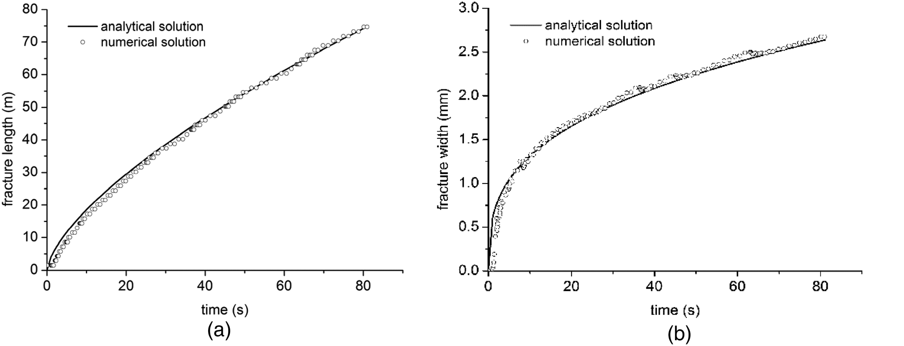
The result comparison between numerical solutions and analytical solutions: (a) fracture length; (b) fracture width.

To evaluate the model performance, the relative error curves of fracture length and width to their analytical solutions are plotted in Figure 3. We observe that the value of the relative error is less than 0.5%, which indicates that our finite element model is reliable.

Figure 3.

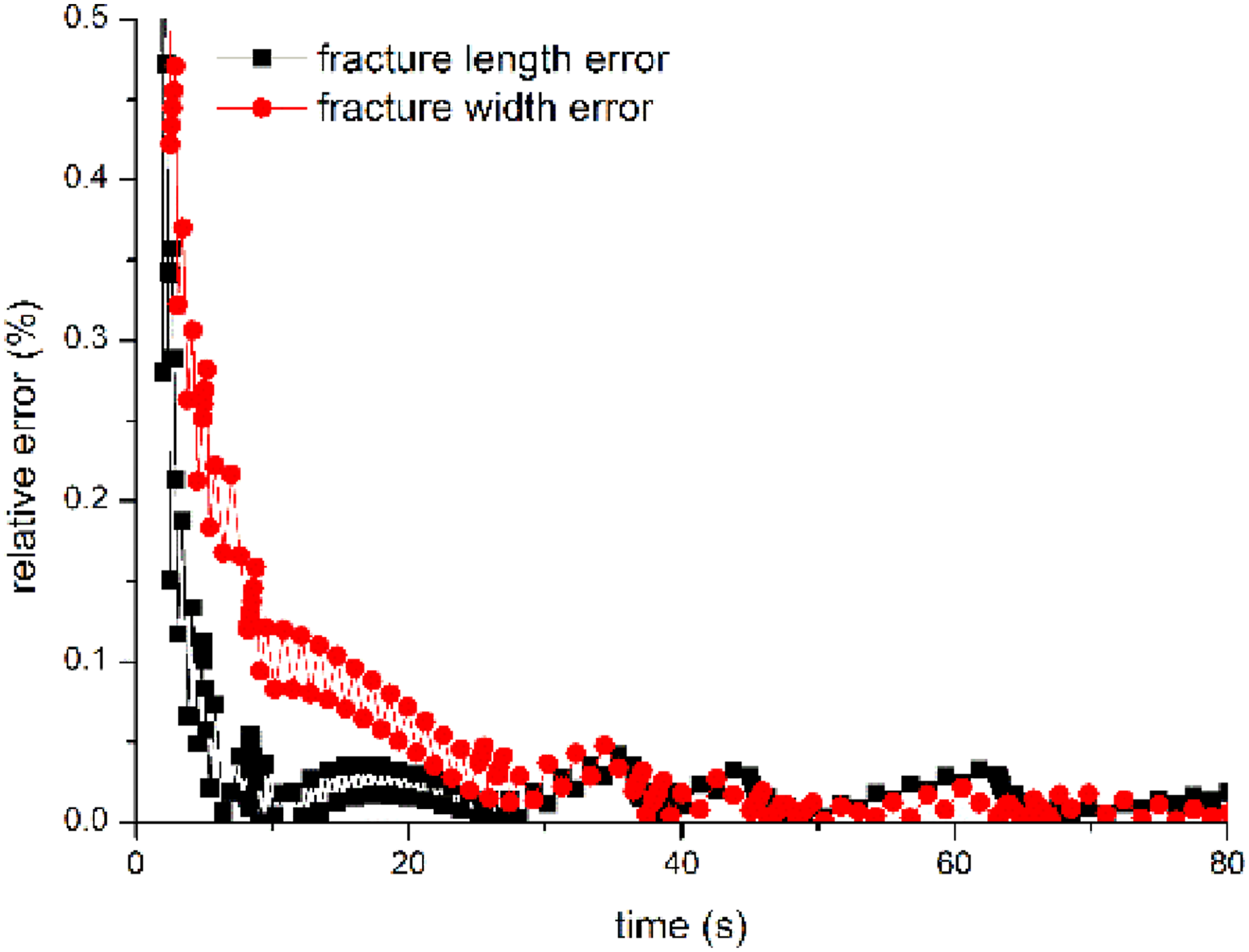
The relative error curve of fracture length and fracture width.

Effect of injection time on fracture closure

The contour plots of the maximum principal stress at different injection times are shown in Figure 4. Figure 4(a) corresponds to the time of instantaneous shut-in (t_ISIP), and Figure 4(b) corresponds to the time of branch fracture closure (t_branch). Thus, Figure 4(b) provides the initial conditions for flow-back analysis. Next, we use the instantaneous shut-in time t_ISIP as the starting time during the flow-back process. The time of major fracture closure is denoted as t_major.

Figure 4.

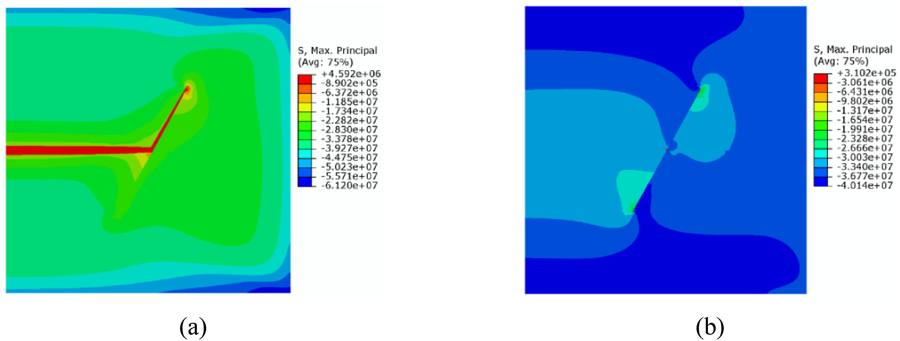
Contour plots of the maximum principal stress at different times: (a) time of instantaneous shut-in; (b) time of branch fracture closure.

Figure 5 presents an elapsed time comparison of the major fracture closure and the branch fracture closure at different approach angles, including 30 degrees, 60 degrees, and 75 degrees. The figure shows that the longer the injection time is, the higher the shut-in pressure is. This is because more fluids are filtrated to the rock matrix normal to the fracture surface, which in turn increases the local pore pressure in the vicinity of the hydraulic fracture. The variation in Figure 5(b) is different from that in Figure 5(b) and 5(c) because the hydraulic fracture patterns are different. Only the upper part of the natural fracture in Figure 5(b) is opened during the interaction between hydraulic fractures and natural fracture. We also observe that there is an inflection point on the curve. The inflection point reflects the fact that the branch fracture is closed during the early stage and the major fracture is closed during the later stage. Thus, fracturing fluid flows from the branch fracture to the major fracture during the flow-back process.

Figure 5.

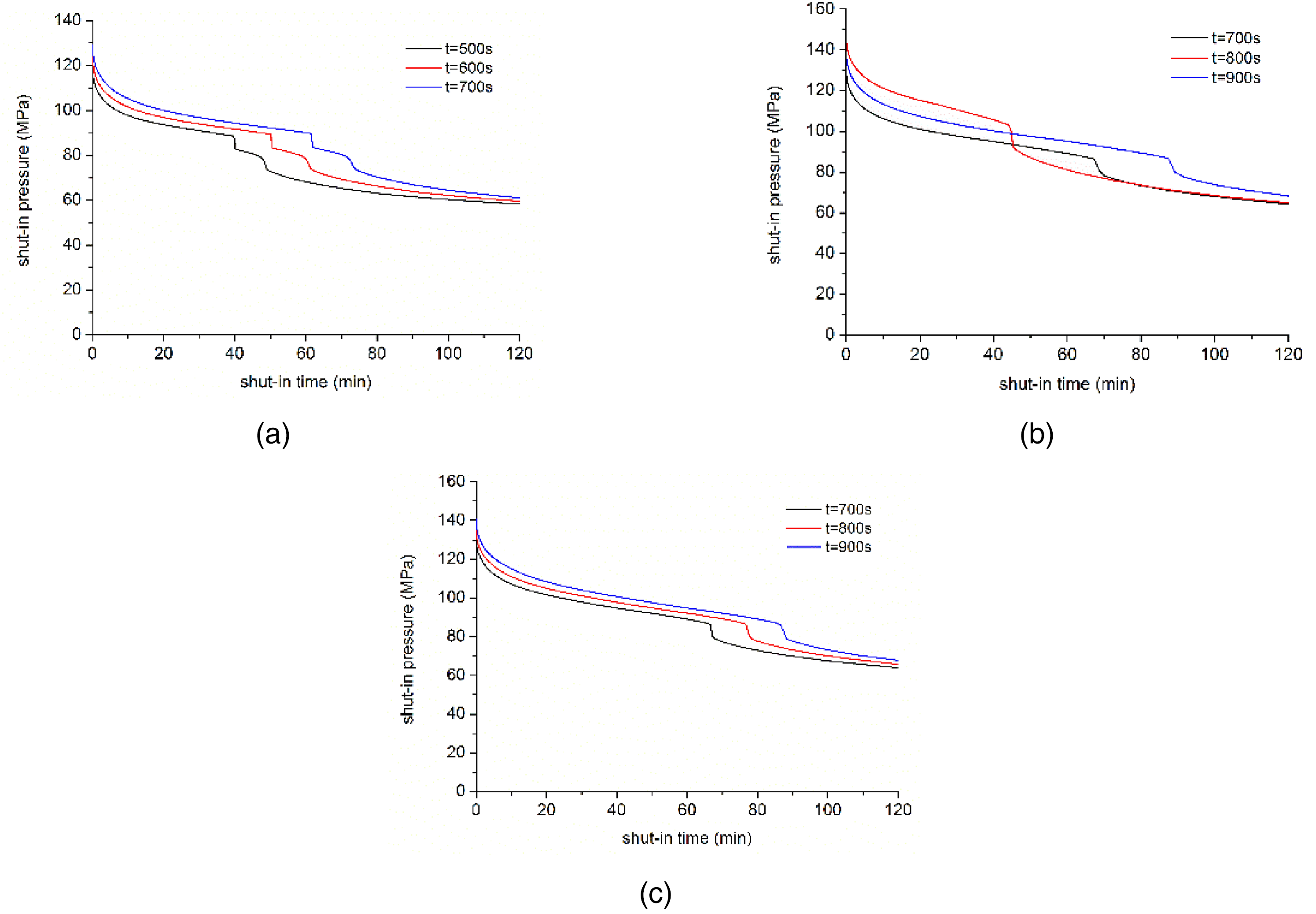
Effect of injection time on fracture closure at different approach angles: (a) β = 30 degrees; (b) β = 60 degrees; and (c) β = 75 degrees.

Figure 6 presents an elapsed time comparison of the major fracture closure and the branch fracture closure at different approach angles. We observe that the longer the injection time is, the higher the ISIP and the closure pressure of the branch fracture are. We also observe that the closure times of the major fracture and the branch fracture, i.e., t_branch-t_ISIP and t_major-t_branch, increase as the injection time increases. Thus, the closure effect of the hydraulic fracture is a slow, gradual process. The closure pressure in the early stage represents the closure of the branch fracture, while the closure pressure in the late stage represents the closure of the major fracture. In addition, the value of t_major-t_branch (red curve) in Figure 4(c) is higher than that of t_branch-t_ISIP, which is different from Figure 4(a) and 4(b). When the intersection angle between hydraulic fracture and natural fracture is high, the opened natural fracture is easy to close during shut-in process under the action of maximum horizontal principal stress.

Figure 6.

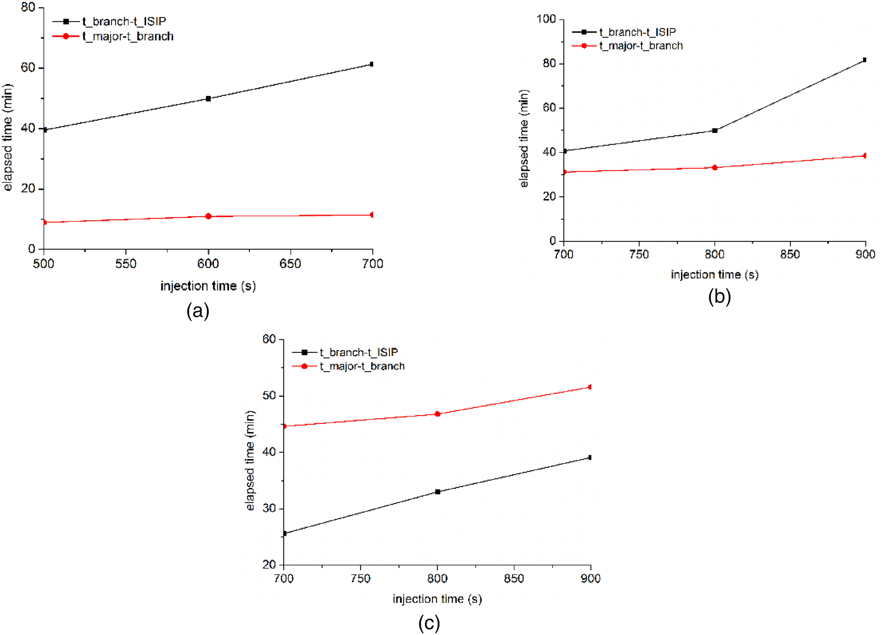
Elapsed time comparison of major fracture closure and branch fracture closure at different approach angles: (a) β = 30 degrees; (b) β = 60 degrees; and (c) β = 75 degrees.

Effect of leak-off rate on fracture closure

Leak-off rate is an important factor during hydraulic fracturing, which impacts the fluid pressure distribution in hydraulic fractures. Figure 7 presents an elapsed time comparison of the major fracture closure and the branch fracture closure at different approach angles, including 30 degrees, 60 degrees, and 75 degrees. The figure shows that the smaller the leak-off rate is, the higher the shut-in pressure is. This is because less fluid is filtrated to the rock matrix normal to the fracture surface, which in turn increases the fluid pressure within the hydraulic fracture. When the value of the leak-off rate is small, the closure time of the branch fracture is obviously delayed and the closure of the major fracture occurs even later.

Figure 7.

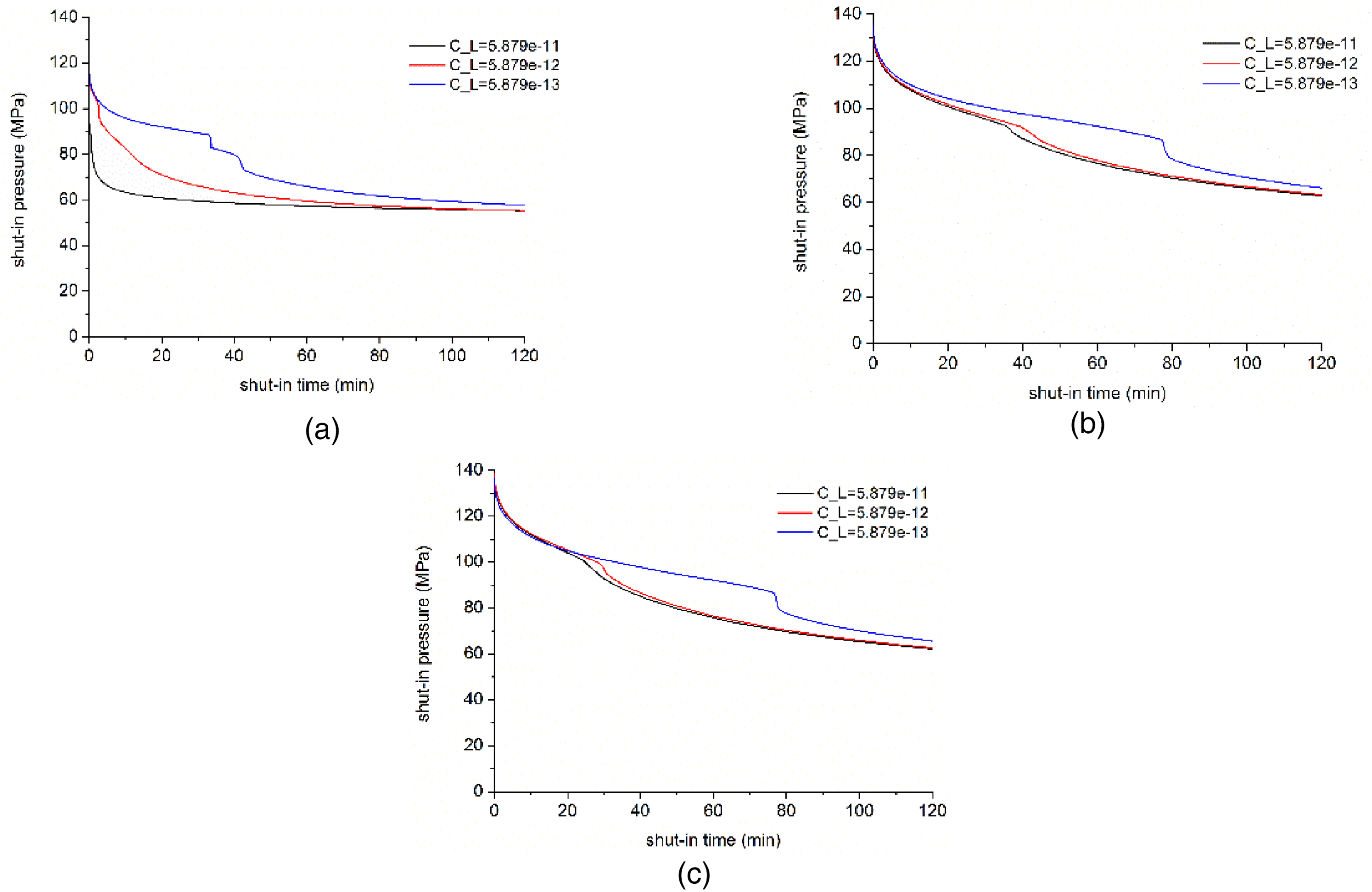
Effect of leak-off rate on fracture closure at different approach angles: (a) β = 30 degrees; (b) β = 60 degrees; and (c) β = 75 degrees.

As shown in Figure 8, an elapsed time comparison of the major fracture closure and the branch fracture closure at different approach angles is plotted. We observe that the leak-off rate has a noticeable effect on the closure time of the branch fracture or the ISIP. The smaller the leak-off rate is, the longer the closure times of the major fracture and the branch fracture are. The smaller the leak-off rate is, the larger the difference between the closure time of the branch fracture and the major fracture is. When the leak-off rate is high, there is little difference between the closure time of the major fracture and that of the branch fracture.

Figure 8.

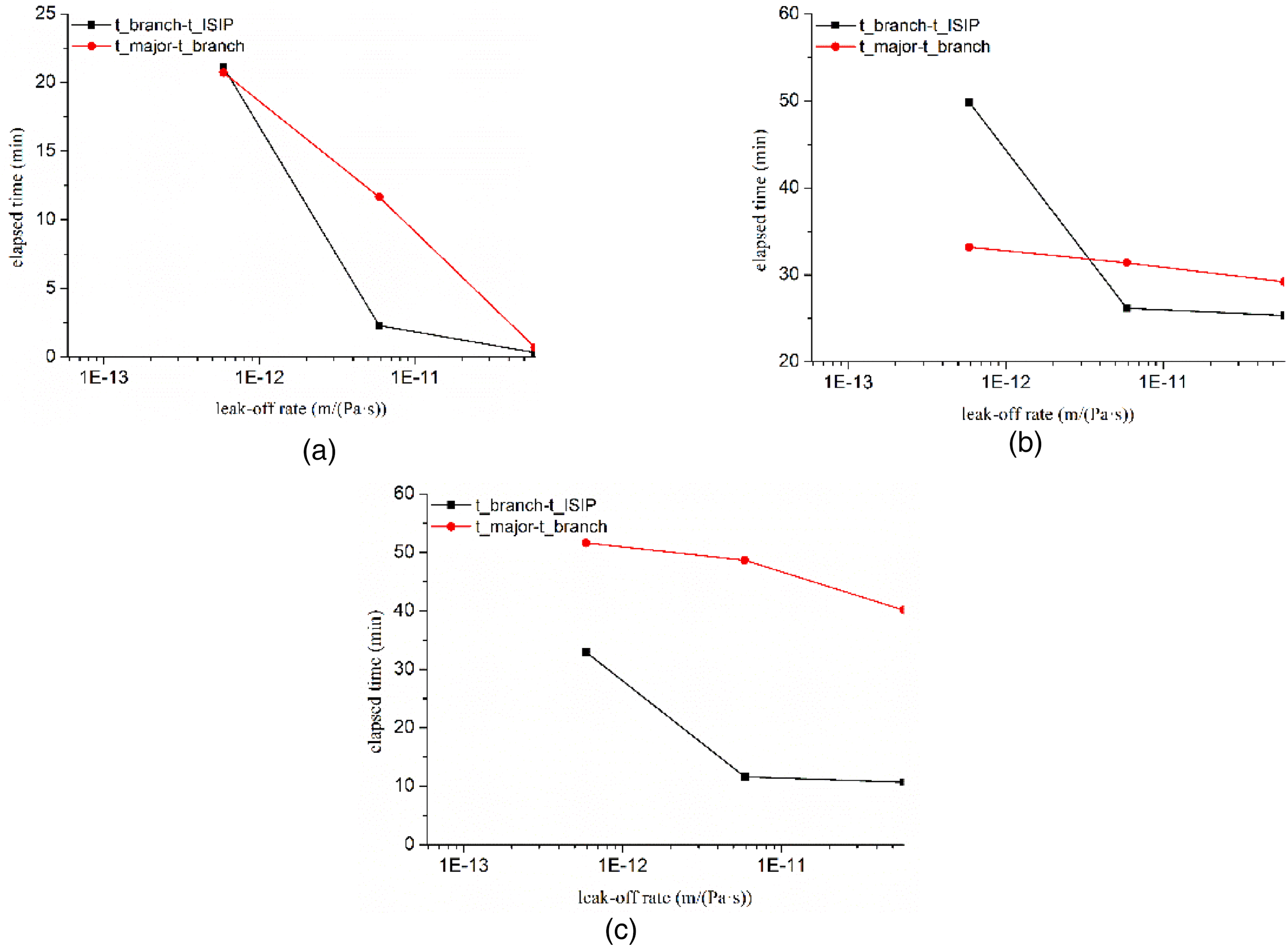
Elapsed time comparison of major fracture closure and branch fracture closure at different approach angles: (a) β = 30 degrees; (b) β = 60 degrees; and (c) β = 75 degrees.

Given the slow leak-off rate and long fracture closure time in tight formations, the fracture closure pressure obtained on site mainly reflects the closure of the branch fracture. Accordingly, the fracture closure pressure cannot be used to determine the minimum horizontal stress. Moreover, the closure pressure of the branch fracture reflects the complexity of the fracture. The larger the difference between the closure pressure of the branch fracture and the minimum stress, the more complex the fracture is considered to be.

Effect of horizontal stress difference on fracture closure

Horizontal stress difference impacts the interaction between hydraulic fracture and natural fractures, and thus effect of horizontal stress difference on fracture closure is investigated in this section. Figure 9 presents an elapsed time comparison of the major fracture closure and the branch fracture closure at different approach angles, including 30 degrees, 60 degrees, and 75 degrees. The figure shows that the larger the horizontal stress difference is, the lower the shut-in pressure is. We also observe that the larger the horizontal in-situ stress difference is, the longer the closure time of the branch fracture is.

Figure 9.

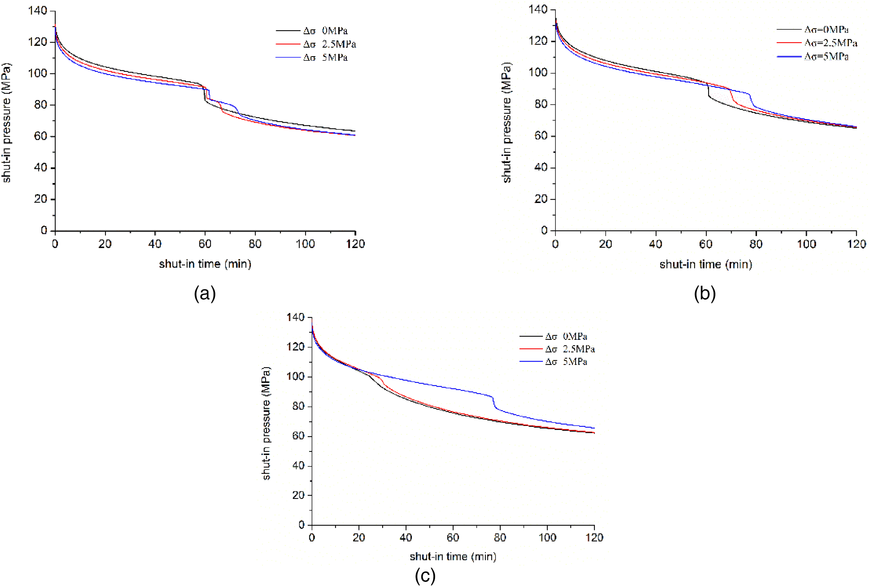
Effect of horizontal stress difference on fracture closure at different approach angles: (a) β = 30 degrees; (b) β = 60 degrees; and (c) β = 75 degrees.

Figure 10 presents an elapsed time comparison of the major fracture closure and the branch fracture closure at different approach angles. We observe that as the horizontal principal stress difference increases, the ISIP decreases and the branch fracture closure pressure increases. We also observe that the larger the horizontal stress difference is, the shorter the closure time of the branch fracture and the longer the closure time of the major fracture are. In the case of a 75-degree approach angle (Figure 8(c)), there is a certain critical stress difference (3.5 MPa). To the left of the critical point, the closure time of the branch fracture is longer than the closure time of the major fracture; to the right of the critical point, the closure time of the major fracture is longer than the closure time of the branch fracture.

Figure 10.

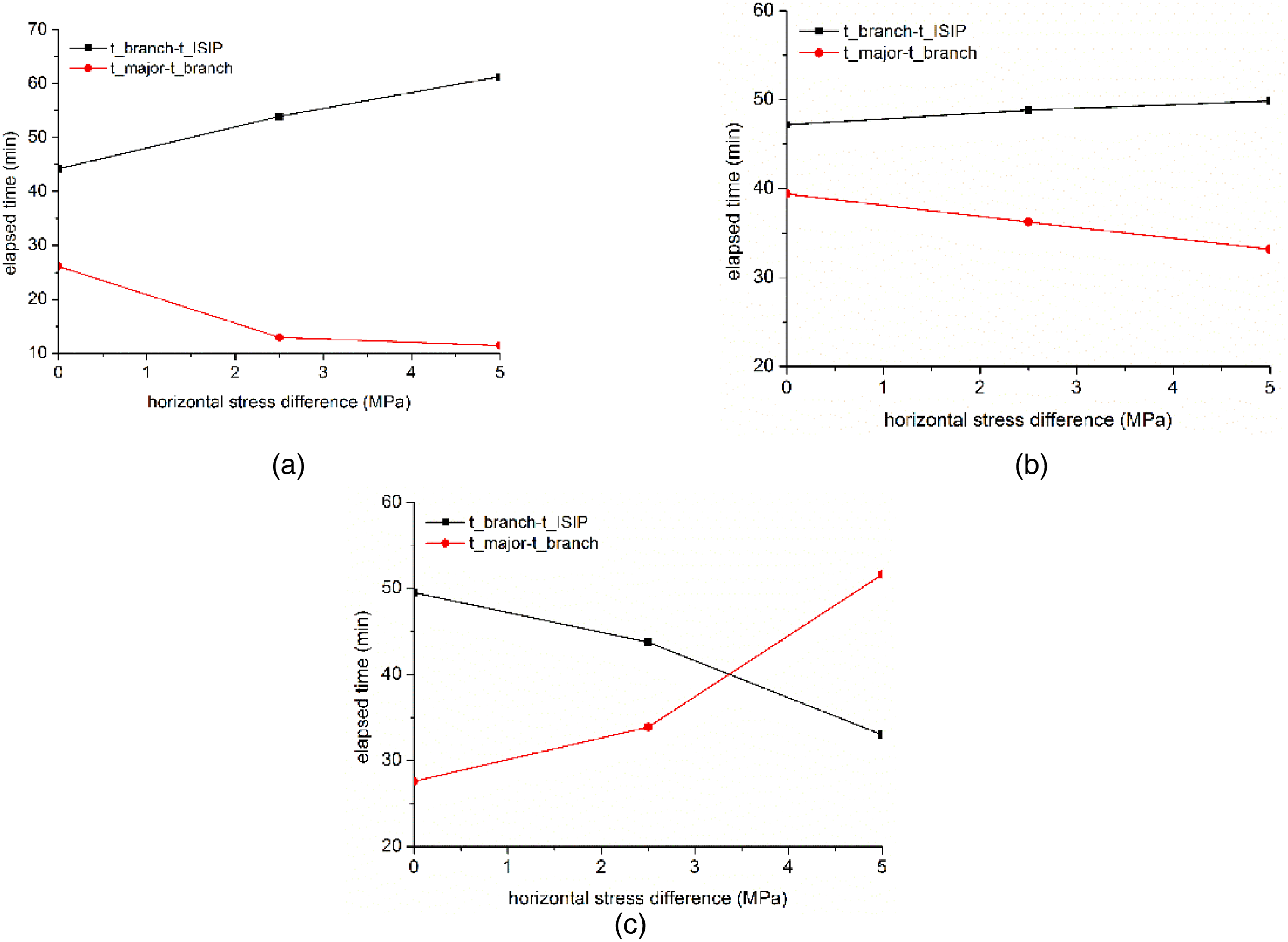
Elapsed time comparison of major fracture closure and branch fracture closure at different approach angles: (a) β = 30 degrees; (b) β = 60 degrees; and (c) β = 75 degrees.

Discussion

Natural fractures widely exist in unconventional reservoirs such as shale gas, shale oil and tight sandstone reservoirs. Natural fractures mainly include cemented and partially uncemented natural fractures. Our investigation aims at the formation with fully cemented natural fractures. Our previous investigation show that the reservoir with an uncemented or partially cemented natural fracture have stronger formatiom capcity of complex fracture than a cemented natural fracture (Wang et al., 2018a; Wang et al., 2021a). Thus, the pressure decline response during hydraulic fracturing of cemented natural fracture is different from that of uncemented or partially cemented natural fractures. Futher investigation of the effect of uncemented or partially cemented natural fractures on fracture closure can be done in the next step.

Conclusion

This paper numerically investigated complex fracture closure pressure during shut-in. The CZM-based finite element model was used to determine the fracture closure pressure and minimum horizontal principal stress of the major hydro-fracture and the branch fracture based on pressure fall-off analysis. The effects of key factors including leak-off rate, injection time, and stress anisotropy on fracture closure process were discussed in detail. The main conclusions are as follows:

The closure times of the major fracture and the branch fracture increase as the injection time increases. Fracture closure is a slow process, and the early closure pressure represents the closure of the branch fracture, which is much higher than the minimum horizontal stress.

The smaller the leak-off rate is, the longer the closure times of the major fracture and the branch fracture are. When the leak-off rate is high, there is little difference between the closure time of the major fracture and that of the branch fracture.

Due to slow reservoir filtration and long fracture closure times, the fracture closure pressure obtained on site mainly reflects the closure of the branch fracture. Accordingly, it cannot be used to determine the minimum horizontal stress. Moreover, the closure pressure of the branch fracture reflects the complexity of the fracture.

The larger the horizontal stress difference is, the shorter the closure time of the branch fracture and the longer the closure time of the major fracture are.

Footnotes

Declaration of conflicting interests

The author(s) declared no potential conflicts of interest with respect to the research, authorship, and/or publication of this article.

Funding

The author(s) disclosed receipt of the following financial support for the research, authorship, and/or publication of this article: Bo Yu was supported by the Key Project of the National Natural Science Foundation of China (Grant No. 51936001); Daobing Wang was supported by the Youth Science Fund of the National Natural Science Foundation of China (Grant No. 51804033) and the General Program Project of the Natural Science Foundation of Beijing (Grant No. 3222030); Dongliang Sun was supported by the Award Cultivation Foundation from Beijing Institute of Petrochemical Technology (Project No. BIPTACF-002)

ORCID iD

Daobing Wang

References

Barenblatt

(1962) The mathematical theory of equilibrium cracks in brittle fracture. In: Dryden

von Kármán

Kuerti

et al. (eds) Advances in Applied Mechanics. San Diego, CA: Elsevier, pp. 55–129. DOI: 10.1016/S0065-2156(08)70121-2

Barree

Craig

(2007) Holistic fracture diagnostics. In: Rocky Mountain Oil & Gas Technology Symposium, 16 April 2007. OnePetro. DOI: 10.2118/107877-MS.

Barree

Miskimins

Gilbert

(2014) Diagnostic fracture injection tests: Common mistakes, misfires, and misdiagnoses. In: SPE Western North American and Rocky Mountain Joint Meeting, 17 April 2014. OnePetro. DOI: 10.2118/169539-MS.

Barree

Mukherjee

(1996) Determination of pressure dependent leakoff and its effect on fracture geometry. In: All Days, Denver, Colorado, 6 October 1996, p. SPE-36424-MS. SPE. DOI: 10.2118/36424-MS.

Belyadi

Fathi

Belyadi

(2019) Hydraulic Fracturing in Unconventional Reservoirs. Cambridge, MA Elsevier. DOI: 10.1016/C2018-0-01643-6.

Benzeggagh, M. L., and M. Kenane, “Measurement of Mixed-Mode Delamination Fracture Toughness of Unidirectional Glass/Epoxy Composites with Mixed-Mode Bending Apparatus,” Composites Science and Technology, vol. 56, pp. 439–449, 1996.

Biot

(1941) General theory of three–dimensional consolidation. Journal of Applied Physics 12(2): 155–164.

Cai

Dahi Taleghani

(2021) Axial fracture initiation during diagnostic fracture injection tests and Its impact on interpretations. Rock Mechanics and Rock Engineering 54(11): 5845–5865.

Carpenter

(2021) Diagnostic fracture injection test analysis method addresses layered rocks. Journal of Petroleum Technology 73(02): 54–55.

10.

Carter

(1957) Derivation of the general equation for estimating the extent of the fractured area. Appendix I of “Optimum Fluid Characteristics for Fracture Extension,” Drilling and Production Practice, GC Howard and CR Fast, New York, New York, USA, American Petroleum Institute: 261–269.

11.

Chipperfield

(2006) After-Closure analysis To identify naturally fractured reservoirs. SPE Reservoir Evaluation & Engineering 9(01): 50–60.

12.

Craig

Eberhard

Barree

(2000) Adapting high permeability leakoff analysis to low permeability sands for estimating reservoir engineering parameters. In: SPE Rocky Mountain Regional/Low-Permeability Reservoirs Symposium and Exhibition, 12 March 2000. OnePetro. DOI: 10.2118/60291-MS.

13.

Dahi Taleghani

Cai

Pouya

(2020) Fracture closure modes during flowback from hydraulic fractures. International Journal for Numerical and Analytical Methods in Geomechanics 44(12): 1695–1704.

14.

Dahi Taleghani

Gonzalez

Puyang

, et al. (2013) Post-treatment assessment of induced fracture networks. Proceedings - SPE Annual Technical Conference and Exhibition 4: 3255–3266.

15.

de Pater

Desroches

Groenenboom

, et al. (1996) Physical and numerical modeling of hydraulic fracture closure. SPE Production & Facilities 11(02): 122–128.

16.

Eltaleb

Rezaei

Soliman

, et al. (2021) A signal processing approach for analysis of fracture injection test in geothermal reservoirs: A case study on the utah FORGE formation. In: SPE Hydraulic Fracturing Technology Conference and Exhibition, 27 April 2021. OnePetro. DOI: 10.2118/204164-MS.

17.

Geertsma

De Klerk

(1969) A rapid method of predicting width and extent of hydraulically induced fractures. Journal of Petroleum Technology 21(12): 1571–1581.

18.

Cheng

, et al. (2017) A semianalytical methodology To diagnose the locations of underperforming hydraulic fractures through pressure-transient analysis in tight Gas reservoir. SPE Journal 22(03): 924–939.

19.

Kholy

Mohamed

Loloi

, et al. (2019) Development of an empirical equation To predict hydraulic-fracture closure pressure from the instantaneous shut-In pressure using subsurface solids-injection data. SPE Journal 24(01): 290–301.

20.

Mayerhofer

Ehlig-Economides

Economides

(1995) Pressure transient analysis of fracture calibration tests. Journal of Petroleum Technology 47(03): 229–234.

21.

McClure

Jung

Cramer

, et al. (2016) The fracture-compliance method for picking closure pressure From diagnostic fracture-injection tests. SPE Journal 21(04): 1321–1339.

22.

McLellan

Janz

(1991) New insights Into fracturing pressure interpretation: case study of minifracture tests in a naturally fractured gas reservoir. Journal of Canadian Petroleum Technology 30(06): 75–84. DOI: 10.2118/91-06-09.

23.

Montgomery

Smith

(2010) Hydraulic fracturing: history of an enduring technology. Journal of Petroleum Technology 62(12): 26–40.

24.

Nolte

(1986) A general analysis of fracturing pressure decline with application to three models. SPE Formation Evaluation 1(06): 571–583.

25.

Nolte

(1991) Fracturing-Pressure analysis for nonideal behavior. Journal of Petroleum Technology 43(02): 210–218.

26.

Plahn

Nolte

Miska

(1997) A quantitative investigation of the fracture pump-in/fIowback test SPE Production & Facilities 12(01): 20–27.

27.

Shiozawa

McClure

(2016) Simulation of proppant transport with gravitational settling and fracture closure in a three-dimensional hydraulic fracturing simulator. Journal of Petroleum Science and Engineering 138: 298–314.

28.

Smith

Montgomery

(2015) Hydraulic Fracturing. Boca Raton: CRC Press, Taylor & Francis Group.

29.

Upchurch

(2003) Determining fracture closure pressure in soft formations using post-closure pulse testing. SPE Production & Facilities 18(04): 230–235.

30.

van Dam

de Pater

Romijn

(2000) Analysis of hydraulic fracture closure in laboratory experiments. SPE Production & Facilities 15(03): 151–158.

31.

Wang

Dong

Sun

, et al. (2020a) A three-dimensional numerical study of hydraulic fracturing with degradable diverting materials via CZM-based FEM. Engineering Fracture Mechanics 237: 107251.

32.

Wang

Shi

Qin

, et al. (2021a) Failure patterns and mechanisms of hydraulic fracture propagation behavior in the presence of naturally cemented fractures. Computer Modeling in Engineering & Sciences 126(3): 891–914.

33.

Wang

Shi

, et al. (2018a) A numerical study on the diversion mechanisms of fracture networks in tight reservoirs with frictional natural fractures. Energies 11(11): 11. Multidisciplinary Digital Publishing Institute: 3035.

34.

Wang

Zhou

, et al. (2018b) The effect of pore pressure on crack propagation in diverting fracturing. In: 52nd U.S. Rock Mechanics/Geomechanics Symposium, 17 June 2018. OnePetro. Available at: https://onepetro.org/ARMAUSRMS/proceedings/ARMA18/All-ARMA18/ARMA-2018-327/122485 (accessed 6 April 2021).

35.

Wang

Zlotnik

Diez

, et al. (2020b) A numerical study on hydraulic fracturing problems via the proper generalized decomposition method. Computer Modeling in Engineering & Sciences 122(2): 703–720.

36.

Wang

Elliott

Sharma

(2021b) Pressure decline analysis in fractured horizontal wells: comparison between diagnostic fracture injection Test Flowback, and Main Stage Falloff. SPE Drilling & Completion 36(03): 717–729.

37.

Zheltov

(1955) Formation of vertical fractures by means of highly viscous liquid. In: 4th World Petroleum Congress, 6 June 1955. OnePetro. Available at: https://onepetro.org/WPCONGRESS/proceedings/WPC04/All-WPC04/WPC-6132/203824.

Complex Fracture Closure Pressure Analysis During Shut-in: A Numerical Study

Abstract

Keywords

Introduction

Method and theory

Numerical simulation

Model verification

Effect of injection time on fracture closure

Effect of leak-off rate on fracture closure

Effect of horizontal stress difference on fracture closure

Discussion

Conclusion

Footnotes

Declaration of conflicting interests

Funding

ORCID iD

References