Sage Journals: Discover world-class research

Abstract

It is important to accurately estimate performances of a hydraulic fractured well, because it will be utilized to evaluate various completion parameters and furthermore to establish a future development plan. Shale gas reservoirs with fracture networks have high initial production rates but show drastic production decline as reservoirs are depleted by production. One of the reasons behind this phenomenon is an increased effective stress during production resulting in fracture closures. Gas mainly flows through hydraulic and natural fracture networks, so the fracture closures cause permeability reduction in the flow areas. In typical hydraulic fracturing operations, proppants are injected with fracturing fluid and placed in the fracture networks. Proppants play a crucial role to keep an induced hydraulic fracture open and retain a well productivity. However, only small portion of the fracture networks are filled with proppants (propped fracture) and the rest exist without proppants (unpropped fracture). Therefore, fracture closures of these regions are quite different. In this article, we have investigated to identify the combined effect of fracture closure and proppant placement on production estimation of a shale gas well. A numerical model has been developed to mimic well performances in Horn River Basin, BC, Canada. We have used pressure-dependent correlations based on experiments to consider fracture permeability alteration with changing reservoir pressure. Proppant placements are described using a fracture propagation model and this enables to classify a whole reservoir into sub regions such as propped, unpropped fracture, and matrix. By comparing with different cases, this article shows that reasonable results on gas production estimation are accomplished when considering fracture closure and proppant placement effects together.

Keywords

Hydraulic fracturing fracture closure proppant placement pressure-dependent permeability shale gas history matching

Introduction

Reservoir characterization is the process of figuring out reservoir parameters of interest by integrating available data. It is essential for decision making and reservoir management. There have been many studies for conventional or channel reservoirs (Jung and Choe, 2012; Kang et al., 2016; Kim et al., 2016; Lee et al., 2014). However, these methods are not easily applicable for shale gas reservoirs with horizontal drilling and multi-stage fracturing.

Hydraulic fracturing jobs have made it possible to economically develop extremely low permeability reservoirs such as shale (Jang and Lee, 2015). Injection pressure above the closure stress of matrix generates hydraulic fractures and dilates pre-existing natural fractures. Created fractures act as a conductive pathway for gas transportation associated with the rock matrix and natural fracture network.

However, shale reservoirs show drastic production declines against conventional reservoirs as the result of fracture closure during reservoir depletion. Although proppants are placed in the fracture networks to avoid fracture closure, experimental studies show that fracture width will be reduced with increasing effective stress. It consequently results in the loss of fracture permeability (Abass et al., 2007; Fredd et al., 2001).

Many experimental studies have been conducted to measure effects of stress on changes of fracture permeability. Fredd et al. (2001) performed laboratory experiments with fractured sandstone cores from east Texas Cotton Valley and presented conductivity variations depending on the proppant concentration and strength. Abass et al. (2007) showed experimental results of stress-dependent permeability for matrix including natural fractures and hydraulic fractures with proppants in a carbonate formation.

Bustin et al. (2008) investigated the permeability of shale cores and concluded that the permeability varies by several orders with effective stress. Chen et al. (2015) derived a correlation between fracture permeability and effective stress and verified the correlation with experimental permeability data from Devonian and Western Canada sedimentary basin shales. They also converted the stress-dependent permeability correlation to a pressure-dependent one under the assumptions of uniaxial strain and constant overburden stress. Above studies are focused on permeability variation of shale rocks by considering the rock with only pre-existing natural fracture not hydraulic fractures.

Besides, simulation studies have been conducted to estimate performances of shale reservoir considering permeability loss due to fracture closure. Ali and Sheng (2015) used a pressure-dependent permeability correlation as a matching parameter and adjusted it for matching of production data from a single well in Haynesville shale, USA. They applied single correlation to the whole fracture networks which means that they did not take into consideration the difference of fracture closure aspects in propped and unpropped regions.

Aybar et al. (2015) constructed a conceptual model composed of one main hydraulic fracture and ten natural fractures and performed systematic simulation analyses. They identified natural and hydraulic fracture closure effects on cumulative gas productions, but this simplified model cannot represent real field productions. Kim et al. (2015) analyzed several key parameters on shale gas production estimation through sensitivity analyses. However, their work was not compared with field production data.

The objective of this article is to develop a numerical model and to match production performances of a well in Horn River Basin, BC, Canada. We first describe fracture network shapes and proppant transports using a fracture propagation model and measured microseismic data. Then, we apply different pressure-permeability correlations in the sub regions. We investigate whether considering both fracture closure and proppant placement together is appropriate for estimating gas productions in the shale gas well.

Theoretical background

Correlation between shale permeability and effective stress

Chen et al. (2015) derived a fracture permeability correlation for shale using fracture porosity ( $Ø_{f}$ ), fracture distribution parameter (D_f), and fracture intensity coefficients (I) as Equation (1)

k = \frac{D_{f} I_{22}}{I_{32}^{3}} \frac{Ø_{f}^{3}}{12}

(1)

where k is the shale permeability and

I_{22}

is the length of fractures per unit area.

I_{32}

is the volume of fractures per unit volume of rock.

They obtained a fracture permeability correlation (Equation (2)) for shale by differentiating Equation (1) with respect to effective stress ( $σ_{e}$ ) and incorporating the definition of fracture compressibility (c_f).

k = k_{0} e - 3 c_{f} (σ_{e} - σ_{e 0})

(2)

where k₀ is the initial permeability and

σ_{e 0}

is the initial effective stress.

Correlation between shale permeability and reservoir pressure

For more rigorous reservoir simulations, changes of stress state should be considered as well as fluid flow. However, because of the complexity and cost of coupled modeling, it is often necessary to simplify these effects in reservoir simulators (Settari et al., 2005). Therefore, it is more practical to correlate fracture permeability to the reservoir pressure to estimate field production behaviors.

A derivation of correlation between the reservoir pressure and permeability starts from the stress–strain relationships.

Δ ɛ_{x} = \frac{1}{E} [Δ σ_{x} - ν (Δ σ_{y} + Δ σ_{z})]

(3)

Δ ɛ_{y} = \frac{1}{E} [Δ σ_{y} - ν (Δ σ_{z} + Δ σ_{x})]

(4)

Δ ɛ_{z} = \frac{1}{E} [Δ σ_{z} - ν (Δ σ_{x} + Δ σ_{y})]

(5)

where

Δ σ

Δ ɛ

are the change of normal stress and strain, ν is the Poisson ratio, and

E

is the Young modulus.

In this stage, two assumptions are made.

The reservoir is under uniaxial strain conditions ( $Δ ɛ_{x} = Δ ɛ_{y} = 0)$ .

The overburden stress remains unchanged ( $Δ σ_{v} = 0$ ) during reservoir production.

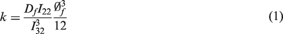
Under uniaxial strain and constant overburden stress conditions (Figure 1), we have

Δ σ_{x} = Δ σ_{y} = \frac{ν}{1 - ν} Δ σ_{z} = \frac{- ν}{1 - ν} α (p - p_{0})

(6)

where α is the Biot constant which ranges from 0 to 1, p and p₀ are the reservoir pressure and initial reservoir pressure, respectively.

Figure 1.

Uniaxial deformation.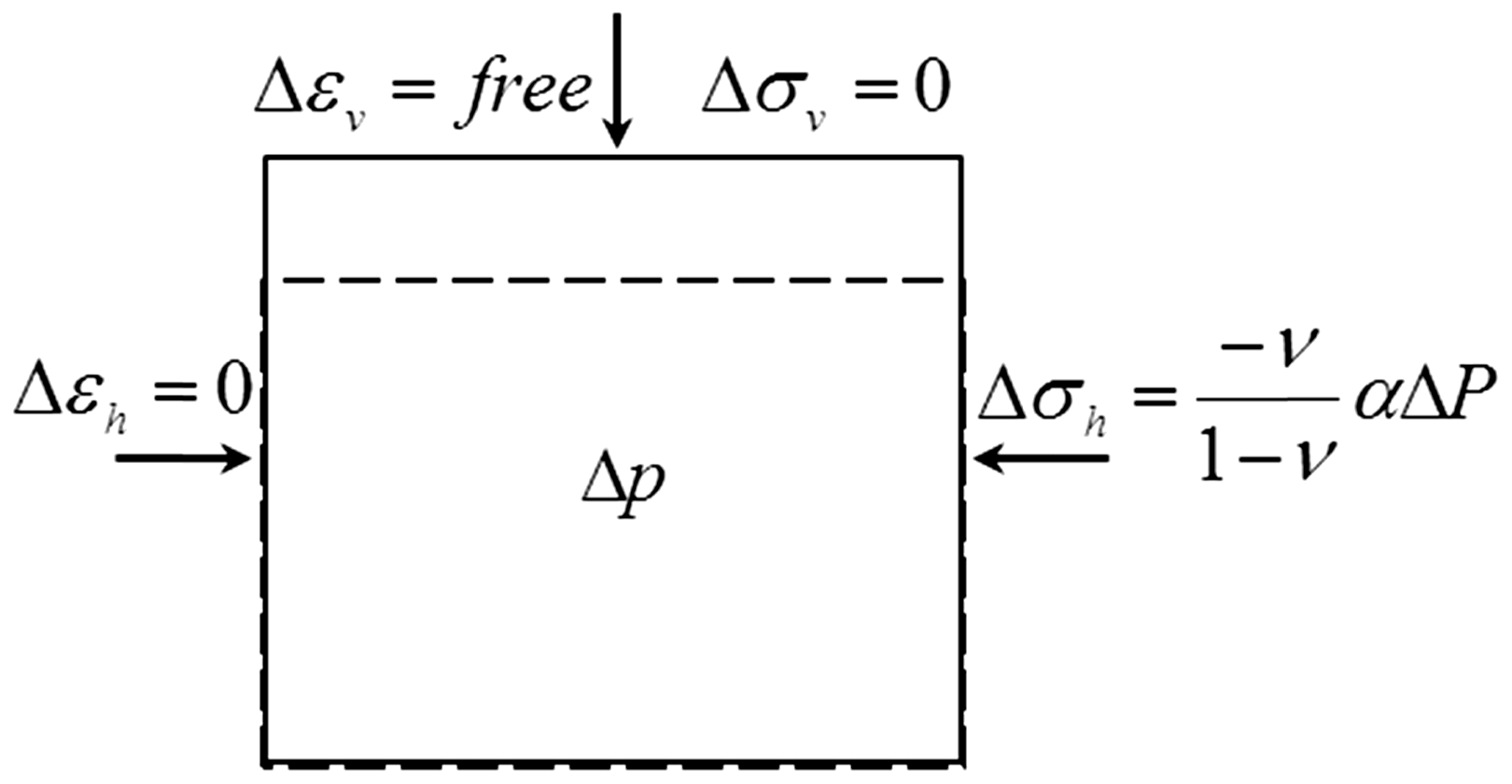

With the assumption that the fracture permeability change is controlled by the mean normal stress ( $σ_{m}$ ), a permeability model can give as the following formula

k = k_{0} e - 3 c_{f} Δ σ_{m} = k_{0} e c_{f} \frac{1 + ν}{1 - ν} α (p - p_{0})

(7)

where

Δ σ_{m}

is the change of mean normal stress.

Unconventional fracture model

An unconventional fracture model (UFM) has recently been developed (Weng et al., 2014), which has special features to simulate fracture propagation, rock deformation, fluid flow, and proppant transport simultaneously during fracturing treatments. Compared to conventional planar fracture models, UFM is able to simulate the interaction of hydraulic fractures with pre-existing natural fractures and to consider the interaction among hydraulic fracture branches by computing the “stress shadow” effect on each fracture exerted by the adjacent fractures.

Figure 2 shows a basic workflow of UFM. At each time step, flow and elasticity equations are solved to derive new pressure and flow distributions in the fracture networks. Injected fluids are modeled as a Power-law fluid and fluid flow along fracture branches is described as

Figure 2.

Basic workflow of an unconventional fracture model (UFM).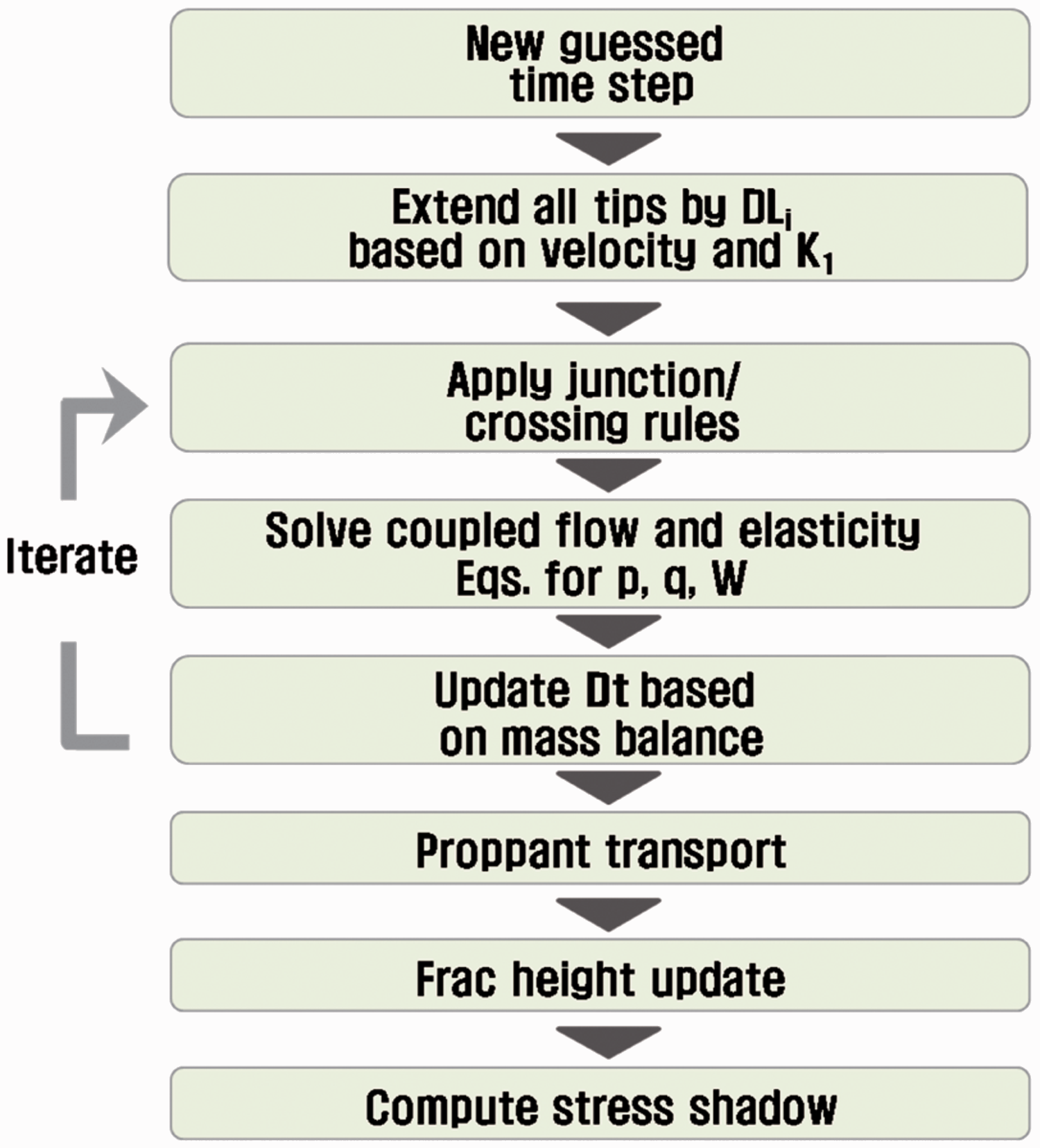

For laminar flow

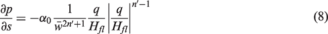
\frac{\partial p}{\partial s} = - α_{0} \frac{1}{\bar{w} 2 n' + 1} \frac{q}{H_{fl}} | \frac{q}{H_{fl}} | n' - 1

(8)

For turbulent flow

\frac{\partial p}{\partial s} = - \frac{f ρ}{\bar{w} 3} \frac{q}{H_{fl}} | \frac{q}{H_{fl}} |

(9)

With

Ø (n') = \frac{1}{H_{fl}} \int_{H_{fl}} (\frac{w (z)}{\bar{w}}) \frac{2 n' + 1}{n'} d z

(10)

where p is the fluid pressure, q is the local flow rate, s is the current position, $\bar{w}$ is the average width of the fracture, $w (z)$ is the fracture width as a function of depth z, $H_{fl}$ is the local height of the fracture occupied by fluid, $n'$ is the Power-law index, f is the Fanning friction factor, and ρ is the fluid density.

Fracture width is calculated using fluid pressure and elastic properties of the rock such as Young’s modulus and Poisson’s ratio through the elasticity equation.

w (z) = \frac{4}{E'} [p_{cp} - σ_{n} + ρ_{f} g (h_{cp} - \frac{h}{4} - \frac{z}{2})] \sqrt{z (h - z)} + \frac{4}{π E'} \sum_{i = 1}^{n - 1} (σ_{i + 1} - σ_{i}) [(h_{i} - z) \cos - 1 h \frac{z (\frac{h - 2 h_{i}}{h}) + h_{i}}{| z - h_{i} |} + \sqrt{z (h - z)} \arccos (\frac{h - 2 h_{i}}{h})]

(11)

where

E'

is the plane modulus,

σ_{i}

is the normal stress in the i-th layer, h_i is the distant from the i-th layer top to bottom tip,

h_{cp}

is the reference depth from the bottom tip, and

p_{cp}

is the fluid pressure at the reference depth.

More detailed description of the governing equations can be found in Weng et al. (2011). Using UFM, Equation (8) or Equation (9) is solved for each component of the fluids and proppant pumped (Figure 3), so proppant placement in the fracture networks can be described after hydraulic fracturing treatment.

Figure 3.

Schematic of proppant transport model.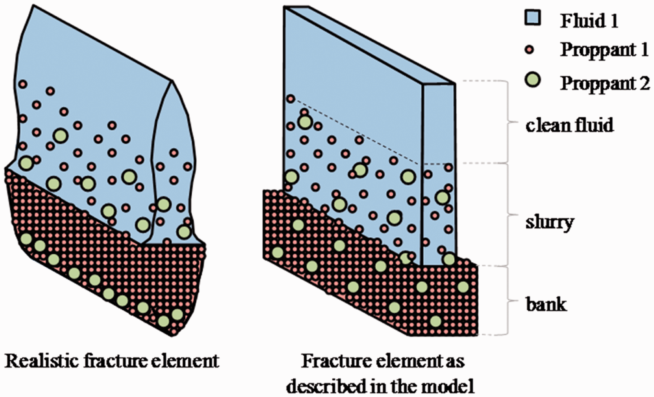

Numerical model construction

In this study, the main target of production estimation is a horizontal shale gas well in Horn River Basin, BC, Canada. Different from conventional reservoirs, unconventional reservoir simulation is focused on the well and the specifics of well completion with a detailed geologic description (Cipolla et al., 2011). We adopt an integrated workflow from a static modeling and carry out fracture simulation for the production estimation in the same platform (Figure 4).

Figure 4.

An integrated workflow of unconventional reservoirs (Cipolla et al., 2011).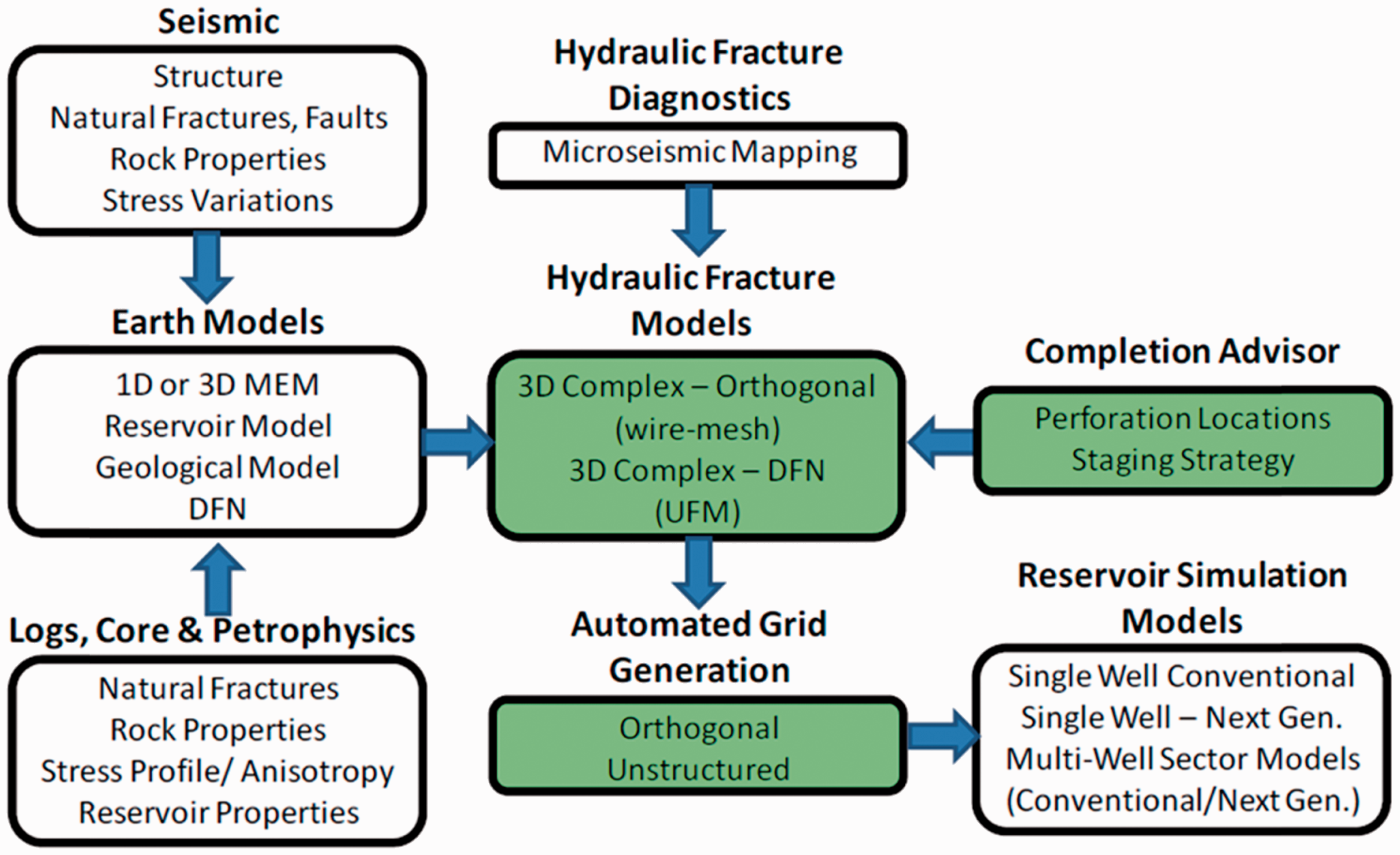

Mechanical earth modeling

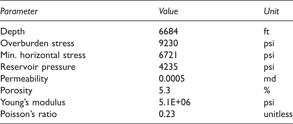
A mechanical earth model (MEM) is defined as a model which describes rock elastic and strength properties, in situ stresses, and pore pressure based on a stratigraphic column (Plumb et al., 2000). In this research, we construct a MEM including formation elastic properties such as Young’s modulus, Poisson’s ratio, and in situ stress states (Figure 5). Equations (12) to (15) are used to derive these properties based on wellbore measurements, microseismic, and geological data. Table 1 lists major parameters and average values of the MEM.

σ_{z} = \int_{0}^{z} ρ (z) g d z

(12)

σ_{h} = (\frac{υ}{1 - υ}) σ_{z} + [1 - (\frac{υ}{1 - υ})] α p

(13)

E = \frac{ρ V_{s}^{2} (3 V_{p}^{2} - 4 V_{s}^{2})}{V_{p}^{2} - V_{s}^{2}}

(14)

ν = \frac{V_{p}^{2} - 2 V_{s}^{2}}{2 (V_{p}^{2} - V_{s}^{2})}

(15)

where

ρ (z)

is the density as a function of depth, g is the gravitational acceleration, and V_p, V_s is the p-wave and s-wave velocity, respectively.

Figure 5.

Distribution of Poisson’s ratio in the mechanical earth model used in this study.

Table 1.

Parameters used in static model.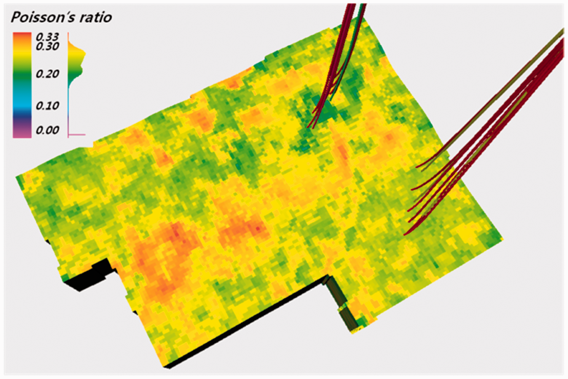

Parameter	Value	Unit
Depth	6684	ft
Overburden stress	9230	psi
Min. horizontal stress	6721	psi
Reservoir pressure	4235	psi
Permeability	0.0005	md
Porosity	5.3	%
Young’s modulus	5.1E+06	psi
Poisson’s ratio	0.23	unitless

Hydraulic fracture modeling

Since created hydraulic fractures play a critical role in each well’s productivity, rigorous estimation of fracture network should be made. A fracture simulation can provide information such as proppant distributions and conductivity of the network.

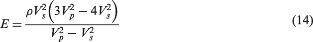
In this research, multi-stage hydraulic fracture treatments are described using UFM and calibrated with microseismic measurements obtained in the field. Figure 6 shows hydraulic fracture simulation results of a target well plotting together with microseismic data. A reasonable match was obtained by adjusting vertical closure stress distributions and horizontal stress anisotropy between microseismic cloud and simulated fracture networks. The fracture networks are then automatically gridded for reservoir simulation presenting various conductivities based on estimated fracture width and proppant placement.

Figure 6.

Fracture simulation results.

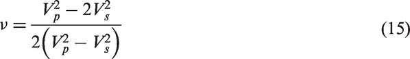
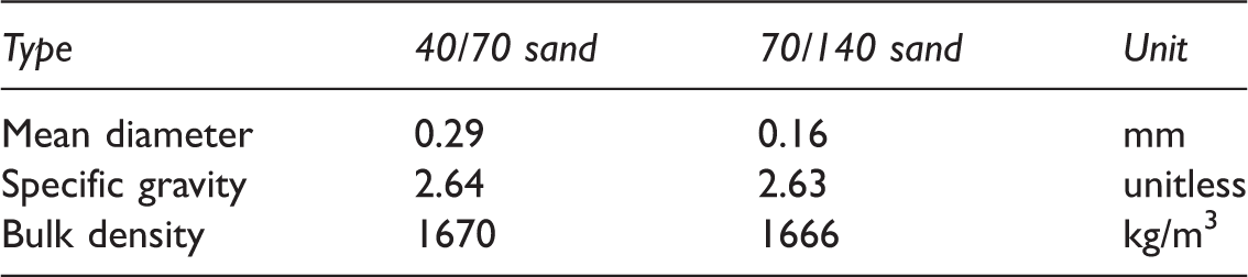
Different sizes of sand are utilized as a proppant for hydraulic fracturing of the well (Table 2). Once the fracture simulation is done, UFM can classify a whole reservoir into separated regions. Figure 7 presents the distribution of the proppants along the hydraulic fractures. The light blue represents proppant placement of 40/70 mesh and the green indicates that of 70/140 mesh. Unpropped fracture region is shown as dark blue and matrix region is given as pink color.

Figure 7.

Proppant placement for the hydraulic fracturing job.

Table 2.

Physical characteristics of proppants used in hydraulic fracturing.

Type	40/70 sand	70/140 sand	Unit
Mean diameter	0.29	0.16	mm
Specific gravity	2.64	2.63	unitless
Bulk density	1670	1666	kg/m³

Derivation of permeability correlation

According to the experiment conducted by Abass et al. (2007), propped and unpropped fractures demonstrate different fracture closure behaviors. Therefore, different pressure-dependent permeability correlations should be applied for each region.

Permeability correlation for the propped region

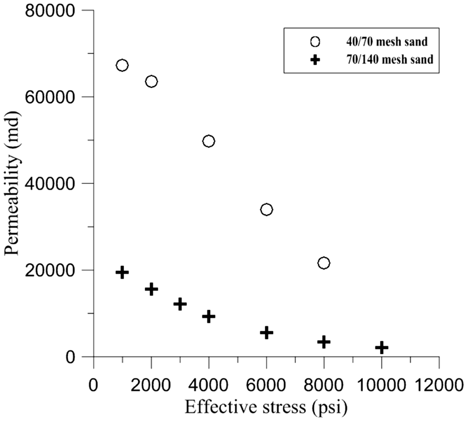
Figure 8 shows stress-dependent permeabilities of 40/70 mesh and 70/140 mesh sands, which are quoted from the Mangrove software database (Schlumberger, 2014). We convert the above correlation into pressure-dependent permeability multipliers, which are more suitable for being used in dynamic simulation. From the assumption that overburden stress is constant, we have

Δ σ_{z} = - α (p - p_{0})

(16)

Figure 8.

Stress-dependent permeability of proppant (from Mangrove database, Schlumberger, 2014).

Converting Equation (16) into an equation of pressure is as follows

p = p_{0} - Δ σ_{z}

(17)

where the Biot constant (

α

) is assumed as 1.

If we regard the effective stress changes as the vertical stress changes, this means stresses in all direction are identical during the experiment. By applying an initial reservoir pressure, we can derive a pressure-dependent permeability multipliers plot as seen in Figure 9(a). The permeability reduction rate is higher in 70/140 mesh case compared to 40/70 mesh case as the well bottom-hole pressure declines.

Figure 9.

Pressure-dependent permeability multipliers. (a) Propped region and (b) unpropped region.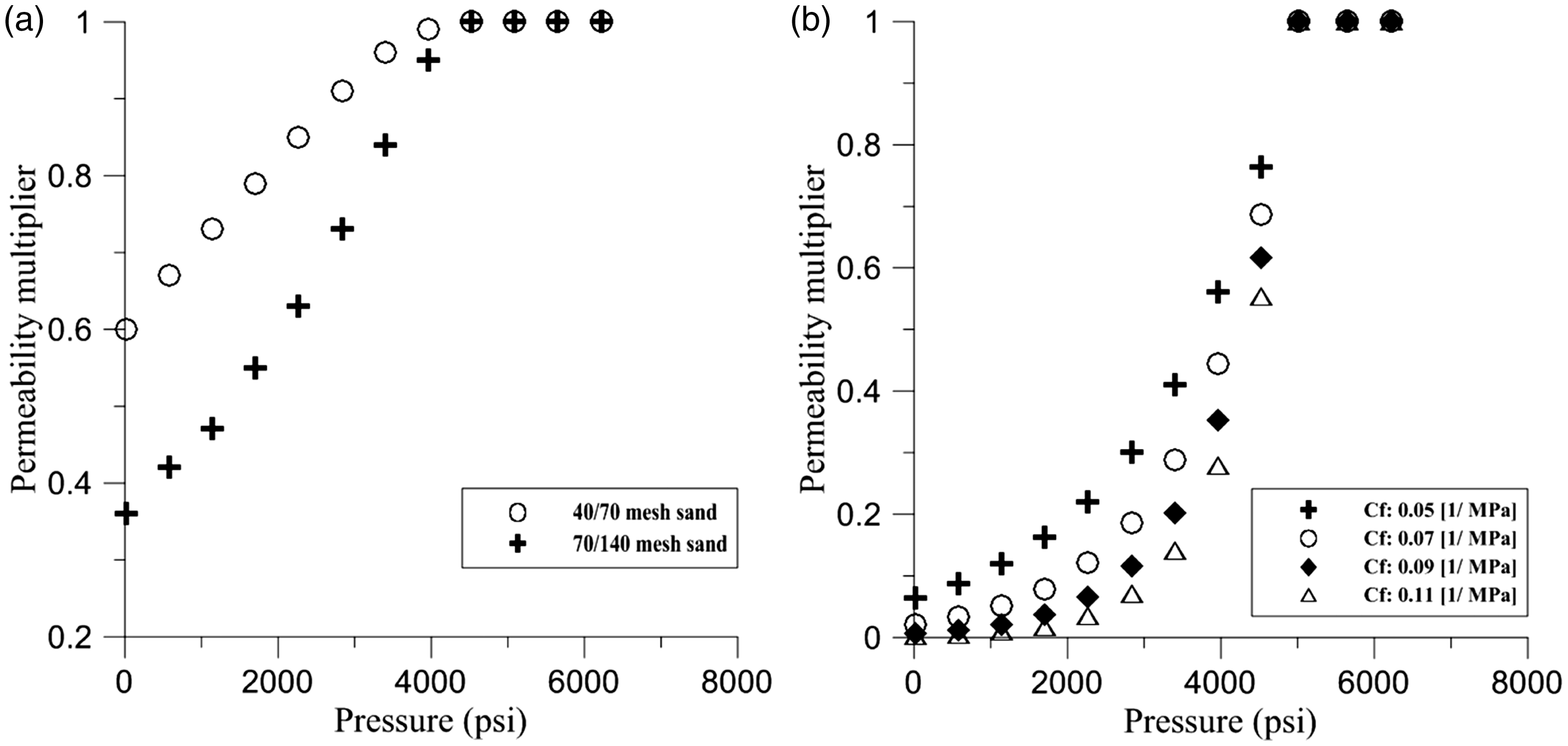

Permeability correlation for unpropped region

For the unpropped fracture and matrix regions, we apply a permeability correlation based on Equation (7). After substituting the initial reservoir pressure and mean Poisson’s ratio into the formula, the only variable remaining is the fracture compressibility. Bustin et al. (2008) suggested that the fracture compressibility ranged from 0.04 to 0.12 MPa⁻¹ according to the quartz contents. In this article, we consider it as an uncertain parameter and make different cases by varying the fracture compressibility: 0.05, 0.07, 0.09, and 0.11 MPa⁻¹. High fracture compressibility means rapid fracture closure as pressure declines (Figure 9(b)).

Results

At first, we construct a base case which does not consider fracture closure effects and compare it with field measured data for daily and cumulative productions (Figure 10). The grey dots indicate measured data and the black solid lines represent simulation results of the base case. It seems to overestimate gas productions because the initial permeability is maintaining unaffected during the whole production period. The other scenario (the black dotted lines) is plotted together in Figure 10, ignoring proppant placement effects. This case underestimates gas productions, because all grids lose their productivity severely during the production. These two are extreme cases of hydraulic fracturing for shale gas productions.

Figure 10.

Simulation results of gas productions. (a) Daily rate and (b) cumulative gas production.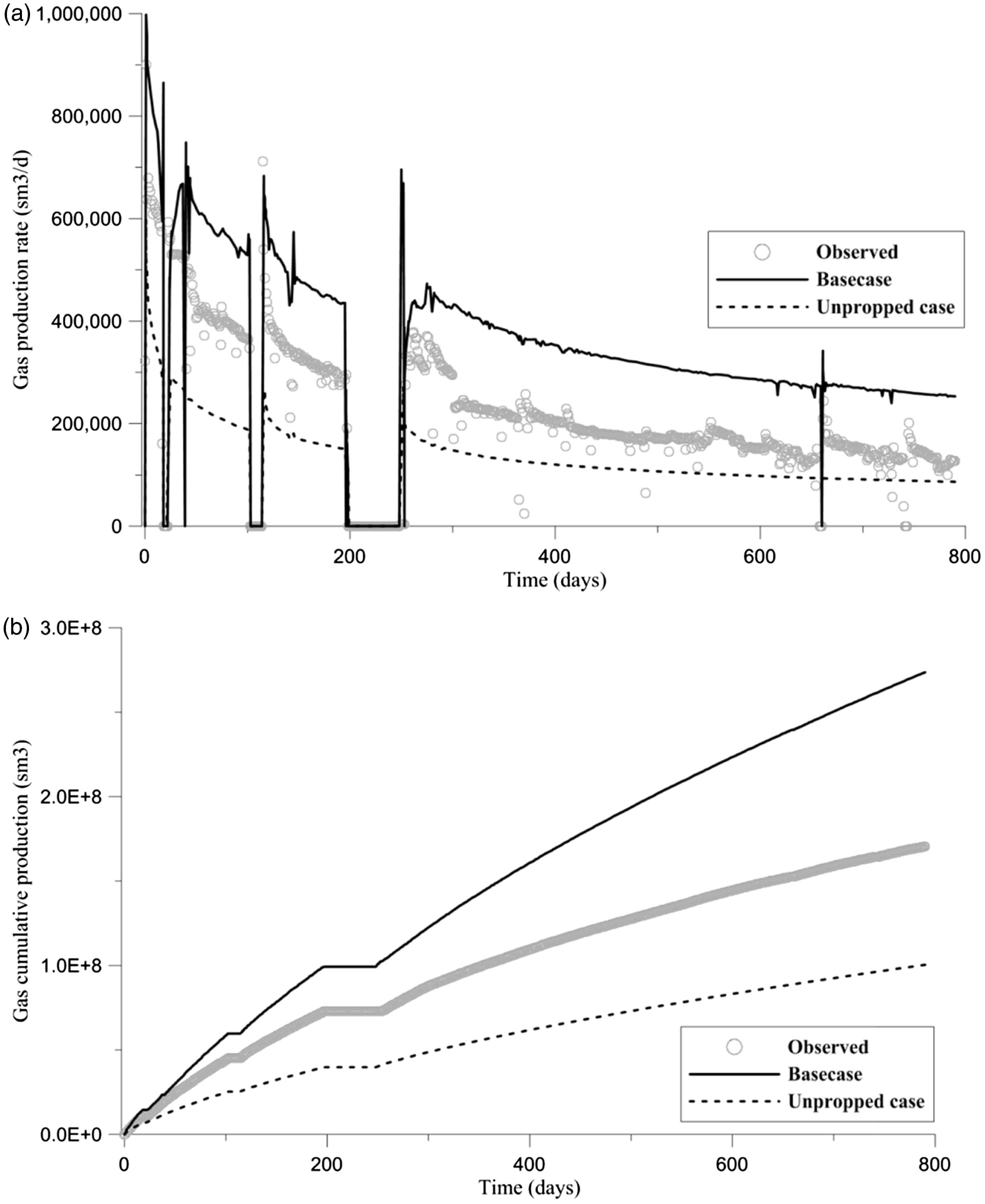

From the above simulation results, we come to a conclusion that the combined effects of fracture closure and proppant placement are critical on production estimations. Therefore, we try to classify the whole reservoir into matrix and fracture regions based on the fracturing simulation results and the more detailed classification is made among the fracture regions: unpropped, 40/70 mesh sand placement, and 70/140 mesh sand placement regions. Then, we apply different permeability correlations for each region.

In this process, the uncertain parameter, the fracture compressibility, is varied from 0.05 to 0.11 MPa⁻¹. At every time step, a reservoir simulator updates the pressure field of the whole grids and re-assigns transmissibility of the grid according to the pressure-dependent permeability multipliers. In this way, changes of permeability could be modeled properly during the production period.

More improved simulation results are obtained in Figure 11, when we consider the effects of fracture closure and proppant placement. Among the four different fracture compressibility cases, we find that the best match is achieved at 0.09 MPa⁻¹. Figures 12 and 13 present matching results of gas productions and tubing-head pressure, respectively. The grey dots indicate field measured data and the black solid lines represent simulation results. A reasonable match of about 800-day production history is obtained.

Figure 11.

Simulation result of gas productions for different fracture compressibilities. (a) Daily rate and (b) cumulative gas production.

Figure 12.

History matched result of gas productions (best case). (a) Daily rate and (b) cumulative gas production.

Figure 13.

History matched result of tubing-head pressure (best case).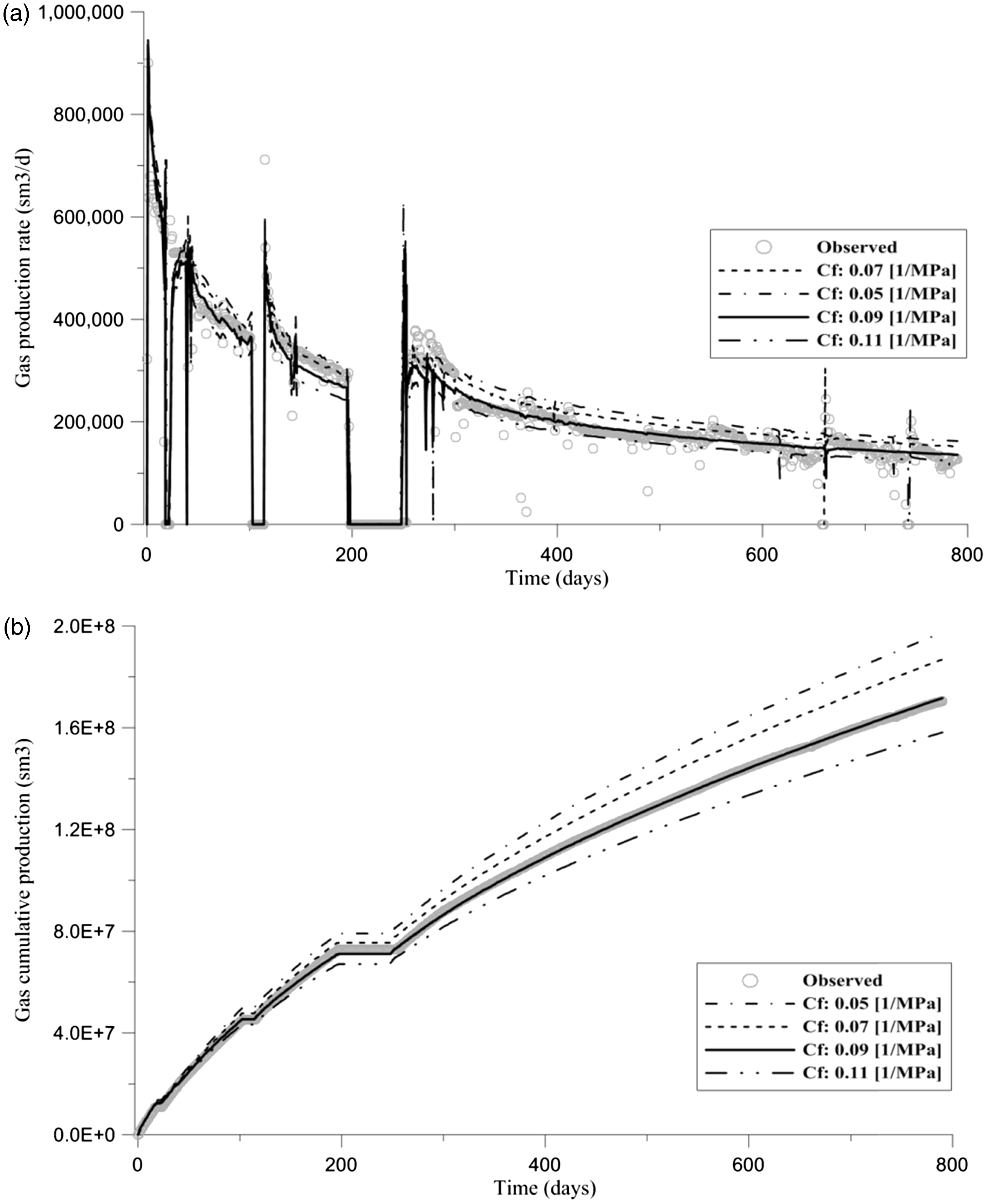

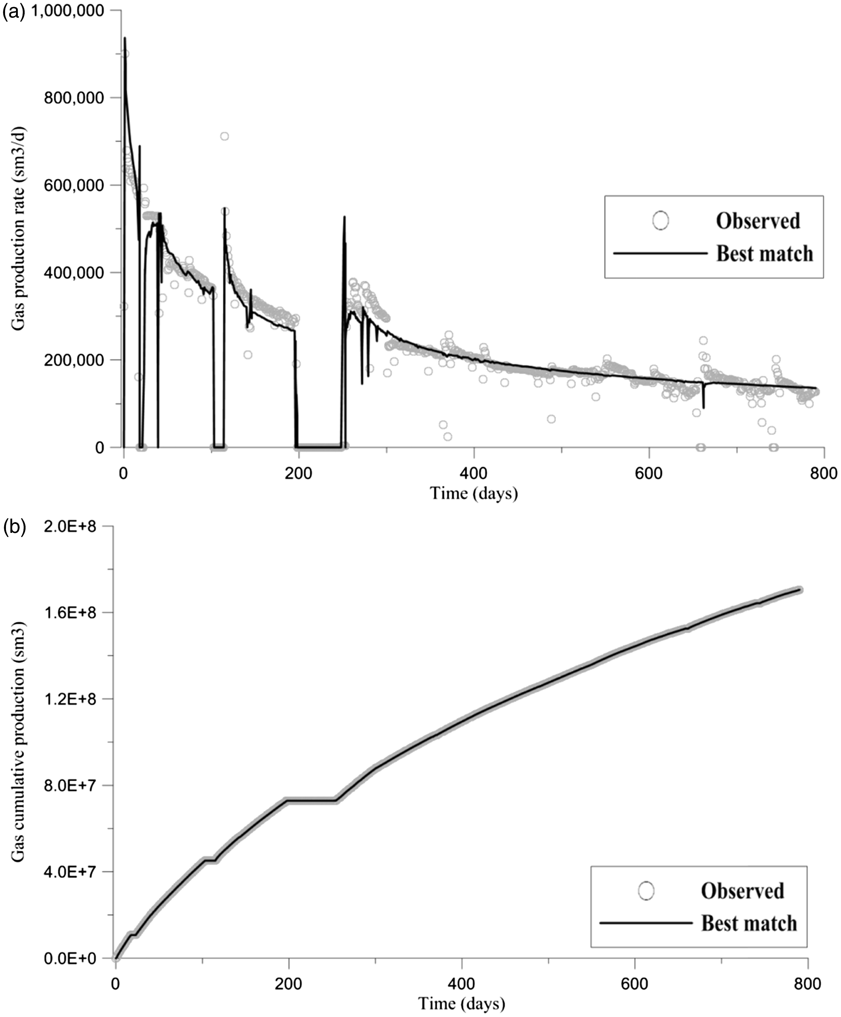
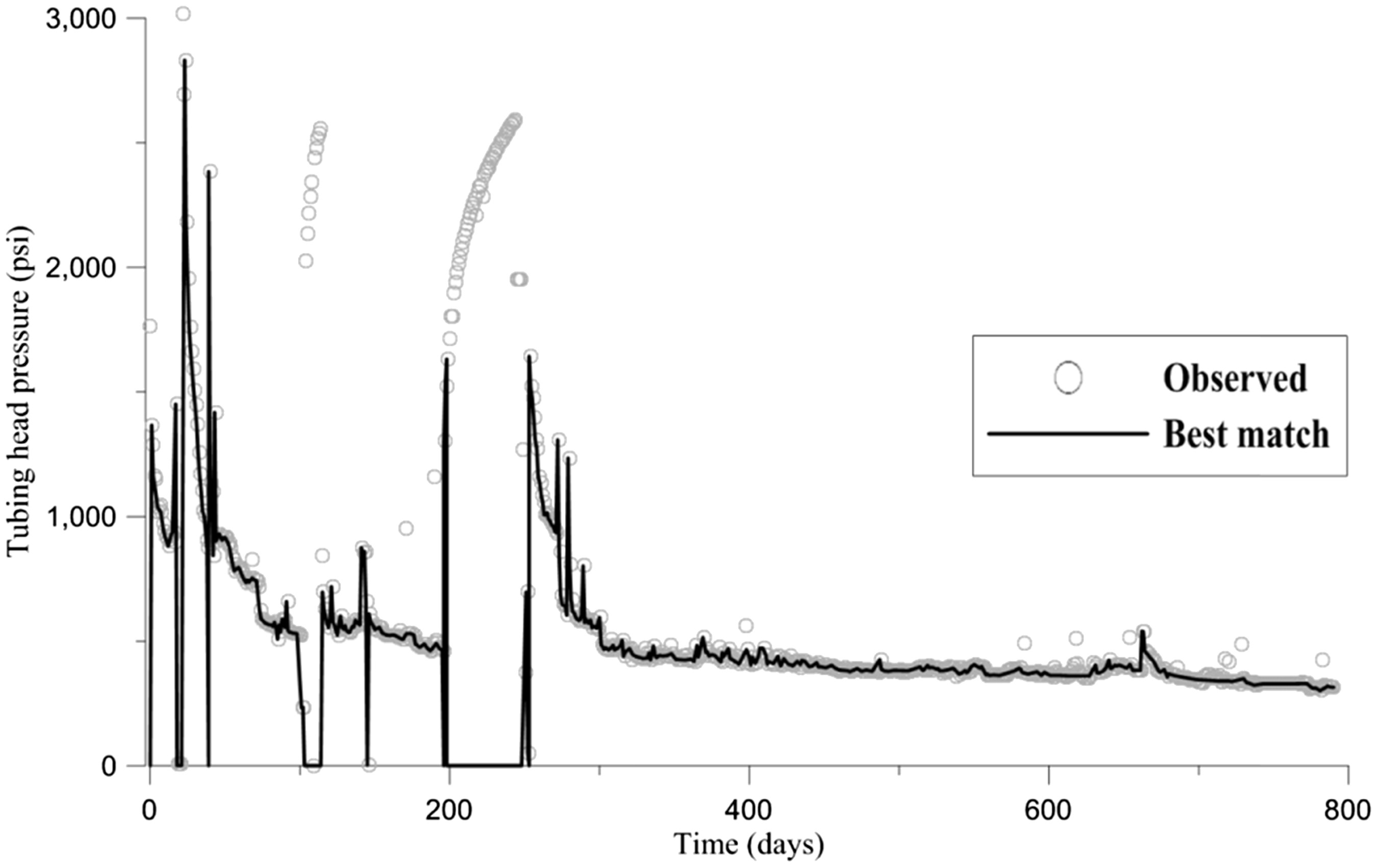
Figure 14 displays pressure distributions at the end of the simulation time. The red colors represent higher pressures, while the blue colors mean lower pressures. From the enlarged view of the pressure distribution near the wellbore (Figure 14(b)), we can observe that pressure declines mainly occurred in the vicinity of the wellbore (∼200 m), which is far less than hydraulic fracture length. If we compare Figure 14(b) with Figure 7, which shows proppant placement in the reservoir, we could find that the initial production mostly comes from free gas in the propped region.

Figure 14.

Pressure distributions at the end of simulation time (790 days). (a) The whole reservoir and (b) vicinity of wellbore.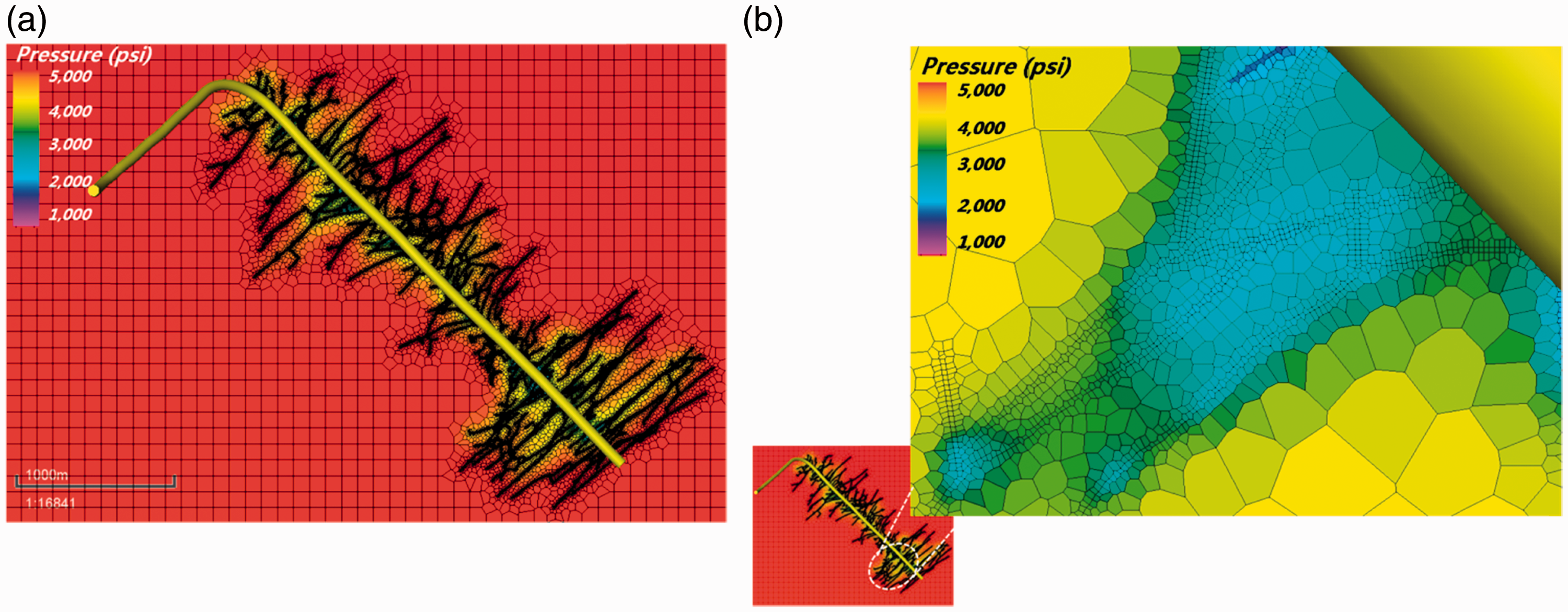

Conclusions

The impacts of fracture closure and proppant placement effects on forecasting shale gas well performances are analyzed using field production data from Horn River shale. The numerical model is constructed based on the integrated workflow for unconventional reservoir. This model can provide information of the fracture network such as proppant distribution and fracture conductivity, which can be a basis for applying different permeability correlations. From this study, we can summarize results as follows:

Pressure-dependent permeability correlations are derived for each region (matrix, fracture: unpropped, proppant types). In the propped regions, well productivity is better retained compared to unpropped regions as reservoir pressure declines.

A good match between field-measured production data and simulation results is accomplished for a well in Horn River shale. From this, we can identify the necessity of considering fracture closure and proppant placement effects on shale gas production forecasting.

In unpropped regions including shale matrix, a high fracture compressibility, which means rapid fracture closure, would be appropriate for reasonable modeling of shale gas production behaviors.

Initial 800-day of production mostly comes from free gas in the propped regions, which can be identified from reservoir pressure distribution. Pressure decline mainly occurs in the vicinity of the wellbore and it is far less than hydraulic fracture length.

Footnotes

Acknowledgments

The authors would like to thank to KOGAS Canada Limited for permission to publish this article. The corresponding author is also thankful to Engineering Research Institute at Seoul National University, Korea.

Declaration of conflicting interests

The author(s) declared no potential conflicts of interest with respect to the research, authorship, and/or publication of this article.

Funding

The author(s) disclosed receipt of the following financial support for the research, authorship, and/or publication of this article: This work was supported by the Energy Efficiency & Resources Core Technology Program of the Korea Institute of Energy Technology Evaluation and Planning (KETEP) granted financial resource from the Ministry of Trade, Industry, & Energy, Republic of Korea (No. 20132510100060).

References

Abass HH, Oritiz I, Khan MR, et al. (2007) Understanding stress dependant permeability of matrix, natural fractures, and hydraulic fractures in carbonate formations. In: SPE Saudi Arabia technical symposium, SPE 110973, Dhahran, Saudi Arabia, 7–8 May, Society of Petroleum Engineers, p.8.

Ali TA and Sheng JJ (2015) Evaluation of the effect of stress-dependent permeability on production performance in shale gas reservoirs. In: SPE eastern regional meeting, SPE 177299, Morgantown, WV, USA, 13–15 October, Society of Petroleum Engineers, p.14.

Aybar

Eshkalak

(2015) Evaluation of production losses from unconventional shale reservoirs. Journal of Natural Gas Science and Engineering 23: 509–516.

Bustin RM, Bustin AMM, Cui A, et al. (2008) Impact of shale properties on pore structure and storage characteristics. In: SPE shale gas production conference, SPE 119892, Fort Worth, TX, USA, 16–18 November, Society of Petroleum Engineers, p.28.

Chen

Pan

(2015) Dependence of gas shale fracture permeability on effective stress and reservoir pressure: Model match and insights. The Science and Technology of Fuel and Energy 139: 383–392.

Cipolla CL, Fitzpatrick T, Williams MJ, et al. (2011) Seismic-to-simulation for unconventional reservoir development. In: SPE reservoir characterization and simulation conference and exhibition, SPE 146876, Abu Dhabi, UAE, 9–11 October, Society of Petroleum Engineers, p.23.

Fredd

McConnell

Boney

(2001) Experimental study of fracture conductivity for water-fracturing and conventional fracturing applications. SPE Journal 6(3): 288–298.

Jang

Lee

(2015) Effect of fracture design parameters on the well performance in a hydraulically fractured shale gas reservoir. Energy Exploration & Exploitation 33(2): 157–168.

Jung

Choe

(2012) Reservoir characterization using a streamline-assisted ensemble Kalman filter with covariance localization. Energy Exploration & Exploitation 30(4): 645–660.

10.

Kang

Lee

Choe

(2016) Improvement of ensemble smoother with SVD-assisted sampling scheme. Journal of Petroleum Science and Engineering 141: 114–124.

11.

Kim K, Ju S, Ahn J, et al. (2015) Determination of key parameters and hydraulic fracture design for shale gas productions. In: The 25-th international offshore and polar engineering conference, ISOPE-I-15-812, Kona, Hawaii, USA, 21–26 June, International Society of Offshore and Polar Engineers, p.7.

12.

Kim

Lee

(2016) Characterization of channelized gas reservoirs using EnKF with application of discrete cosine transformation. Energy Exploration & Exploitation 34: 319–336.

13.

Lee

Jung

Shin

(2014) Uncertainty quantification of channelized reservoir using ensemble smoother with selective measurement data. Energy Exploration & Exploitation 32(5): 805–816.

14.

Plumb R, Edwards S, Pidcock G, et al. (2000) The mechanical earth model concept and its application to high-risk well construction projects. In: IADC/SPC drilling conference, SPE 59128, New Orleans, LA, USA, 23–25 February, Society of Petroleum Engineers, p.13.

15.

Schlumberger (2014) Mangrove Engineered Stimulation Design Database. Houston, TX: Schlumberger Information Solutions.

16.

Settari AT, Bachman RC and Walters DA (2005) How to approximate effects of geomechanics in conventional reservoir simulation. In: SPE annual technical conference and exhibition, SPE 97155, Dallas, TX, USA, 9–12 October, Society of Petroleum Engineers, p.7.

17.

Weng X, Kresse O, Cohen C, et al. (2011) Modeling of hydraulic fracture network propagation in a naturally fractured formation. In: SPE hydraulic fracturing conference and exhibition, SPE 140253, Woodlands, TX, USA, 24–26 January, Society of Petroleum Engineers, p.13.

18.

Weng

Kresse

Chuprakov

(2014) Applying complex fracture model and integrated workflow in unconventional reservoirs. Journal of Petroleum Science and Engineering 124: 468–483.

Efficient production estimation for a hydraulic fractured well considering fracture closure and proppant placement effects

Abstract

Keywords

Introduction

Theoretical background

Correlation between shale permeability and effective stress

Correlation between shale permeability and reservoir pressure

Unconventional fracture model

Numerical model construction

Mechanical earth modeling

Hydraulic fracture modeling

Derivation of permeability correlation

Permeability correlation for the propped region

Permeability correlation for unpropped region

Results

Conclusions

Footnotes

Acknowledgments

Declaration of conflicting interests

Funding

References