CIBSE TM54 energy projections I: A case study using quasi-steady state modelling

Abstract

CIBSE TM54 was recently revised and covers best practice methods to evaluate the operational energy use of buildings. TM54 is a guidance document that can be used for performance evaluation at every stage of the design and construction process, and during the occupied stage, to ensure that long-term operational performance aligns with the design intent. The main performance evaluation principles in TM54 are a step-by-step modelling approach and scenario testing, to improve the robustness of the design proposal calculations. The latest edition of this technical memorandum brings an updated perspective to the modelling approaches, including detailed Heating, Ventilation and Air Conditioning (HVAC) modelling and simulation. It also incorporates more detailed guidance around risks, target setting, scenario testing and sensitivity analysis. A case study approach is used to explore and demonstrate some important aspects described in TM54. TM54 recommends three modelling approaches (aka implementation routes) that a project can follow depending on its scale and complexity: using quasi-steady state tools; dynamic simulation with a template HVAC system; and dynamic simulation with detailed HVAC system modelling. As part of a series of three, this case study provides an application of the first implementation route: modelling using quasi-steady state tools.

Practical Application

This case study provides detailed guidance on undertaking CIBSE TM54 modelling and projecting design stage building performance. The study covers the interpretation and clarifications of how TM54 can be applied, through the quasi-steady-state modelling tools.

Introduction

The Chartered Institution of Building Services Engineers (CIBSE) Technical Memorandum TM54 provides building designers and owners with guidance on how to evaluate operational energy use once a building’s design has been developed. First published in 2013, ¹ this was one of the first pieces of industry guidance documents in the UK to address the performance gap issue and better project operational performance of actual energy use. In the recently published revision, CIBSE TM54: 2022, ² the guidance has been made up to date by taking account of regulatory and industry changes such as the net-zero carbon transition, performance targets and advances in Heating, Ventilation and Air Conditioning (HVAC) modelling.

For a holistic application and wider adoption of best practice energy projections in the industry, the new TM54 document suggests three implementation routes depending on different scales and complexity of projects. The modelling approaches include:

1. Quasi-steady state modelling

2. Dynamic simulation modelling (DSM) using template HVAC systems

3. Dynamic simulation modelling (DSM) using detailed HVAC systems

In this first of three case studies, an example of TM54 design stage building performance modelling for a Passivhaus school building using a steady-state modelling tool is presented. In the first part of this case study, the step-by-step modelling methodology proposed in CIBSE TM54 for the steady-state modelling implementation route is described. Then the case study building is introduced and the modelling inputs and assumptions for each of the TM54 steps are explained. Finally, results are presented as per TM54 requirements including deterministic calculations, sensitivity and scenario assessments, and benchmarking against industry standards.

Methodology

The main performance evaluation principles in TM54 include a step-by-step modelling approach, systematic sensitivity and scenario analysis, and performance reporting including benchmarking, to improve the robustness of the design proposal calculations and provision of advice to clients.

After the selection of the appropriate modelling approach (Step 0), depending on project-specific requirements, step-by-step modelling is undertaken. The modelling approach used in this case study is quasi-steady state modelling. The procedural steps involved as per TM54 are shown in Figure 1. The 17-step modelling methodology has been divided into three stages: baseline model generation, scenario/sensitivity assessments, and result reporting & benchmarking. In the later sections of the case study, the modelling is presented by following these steps, explaining the use of building-specific information in creating a TM54 model.

Figure 1.

Step-by-step approach for quasi-steady state modelling as per TM54 2.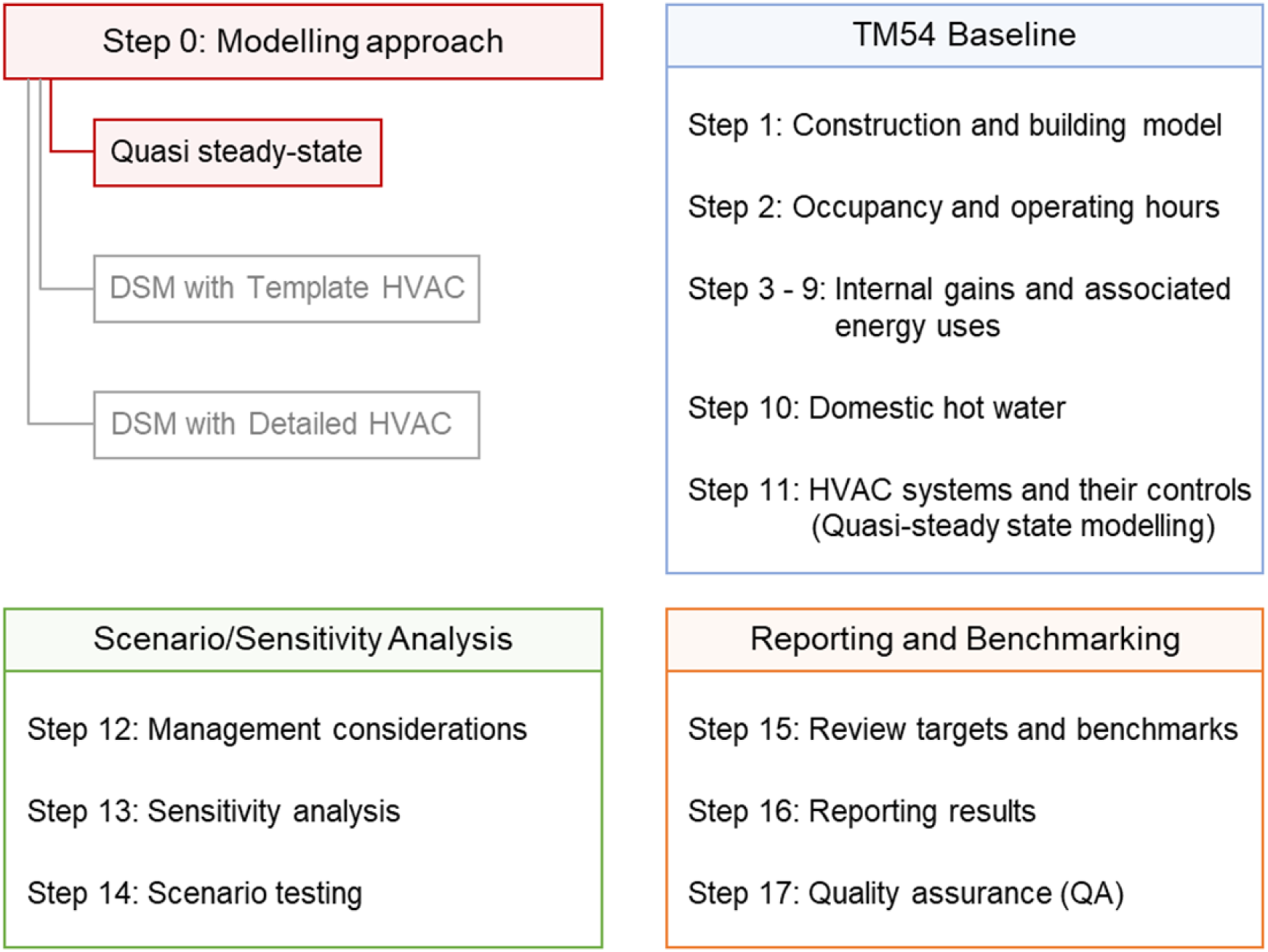

Modelling for TM54 in this case study is undertaken using, the Passive House Planning Package (PHPP) tool. ³ PHPP is used for buildings aiming to achieve Passivhaus certification and represents quasi-steady tools used for the evaluation of energy performance in buildings. PHPP, when used for PassivHaus certification, may use certain standard model inputs. However, in this case study PHPP is used for TM54 modelling and therefore the inputs in the PHPP tool are building-specific. Also, the presentation of building details and the project context follow TM54 steps and may not be in the same workflow as the software itself. Similarly, the results reporting along with process documentation of inclusion or exclusion of any aspects of modelling also follow TM54 requirements. This makes the case study presentation software agnostic and replicable for any project that uses a quasi-steady state modelling approach.

Case study application and modelling approach

The school is approximately 1,500 m² and is located in Trimsaran, Carmarthenshire County in rural Wales. Being a primary school, the two-storey building mainly consists of Classrooms (40%), Circulation/Hub (30%) and halls (15%) with the remaining areas including storage rooms, offices for staff, toilets and kitchen. The school has been designed to meet the Passivhaus standard of energy efficiency and comfort. Passivhaus is an energy standard to achieve the lowest practical heating demand for a building . ⁴ The building meets the standard requirements by having high levels of insulation, triple-glazed windows, and mechanical ventilation with heat recovery (MVHR) among other features. Figure 2 shows the building’s exterior image.

Figure 2.

Case study school building.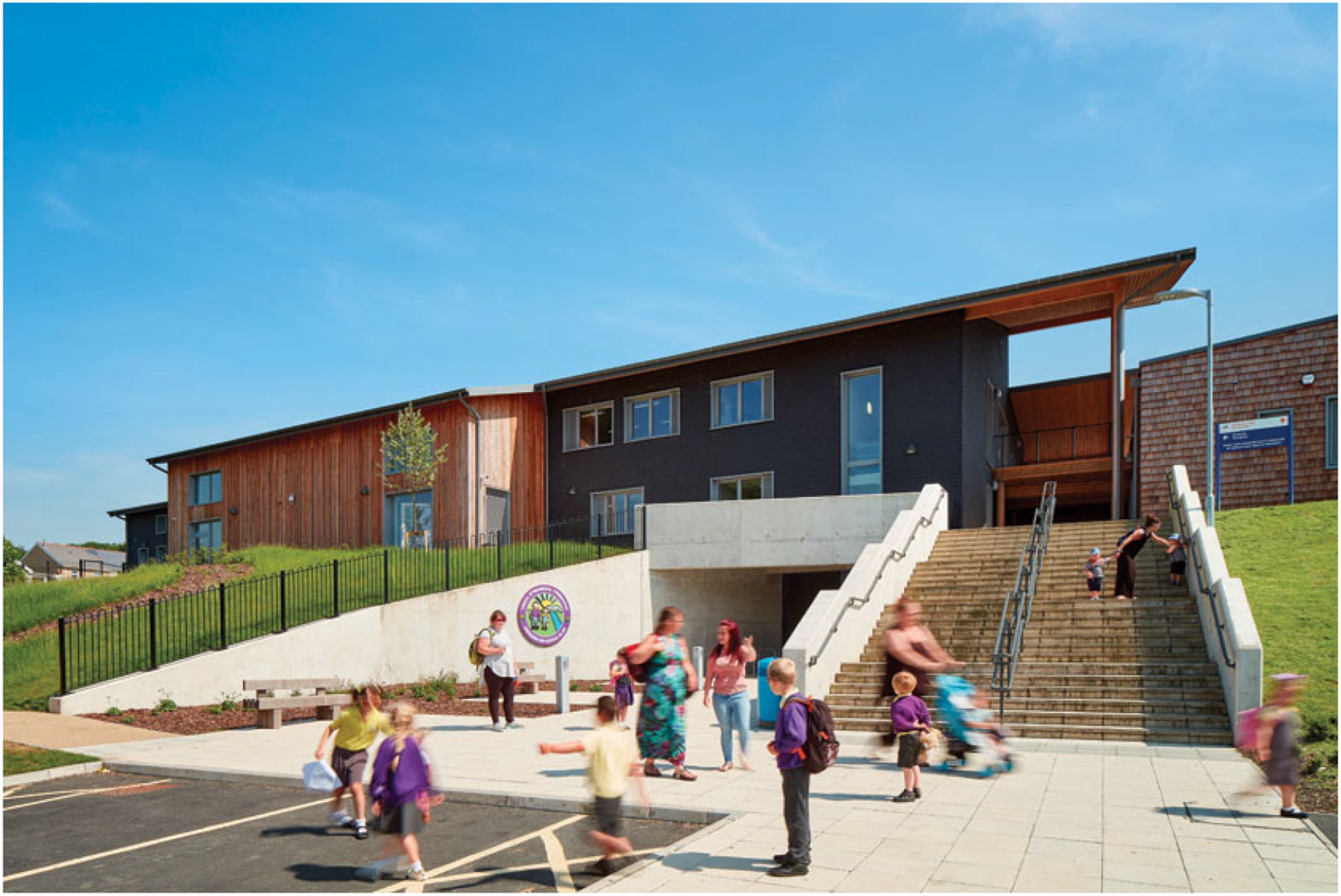

The compact design of this school building with highly insulated envelope and airtightness means that the heat gains/losses are minimised. Additionally, as the building uses simple heating and ventilation systems with predictable operational patterns, it can be assumed that the building energy demand will not vary significantly with hourly external weather. Therefore, it is suggested that a simplified approach to modelling, such as quasi-steady state building energy modelling can be used to develop the TM54 model of this building. Detailed guidance on modelling approaches and tools is explained in TM54. ²

TM54 baseline

The baseline building generation is covered in TM54 Steps 1 – 11 (Figure 1). For each of these steps, model inputs must be defined along with ascertaining confidence levels in the underlying assumptions to guide 5.0 Scenario/Sensitivity analysis.

Geometry and site details

Step 1: Constructing and building the model

Defining the building geometry and setting up the site information in the model is the first step in undertaking building modelling and forms the basis from which all future calculations are undertaken. This process involves setting up building geometry details and areas, defining constructions, zoning, and selecting appropriate weather data. The accuracy and quality of these inputs in the model will in turn affect the accuracy of future model outputs. Contrary to DSM tools, where building geometry and zoning are defined in three dimensions, spreadsheet-based tools such as PHPP require simpler inputs (calculated precisely from the actual drawings) such as overall zone areas and volumes and envelope component details.

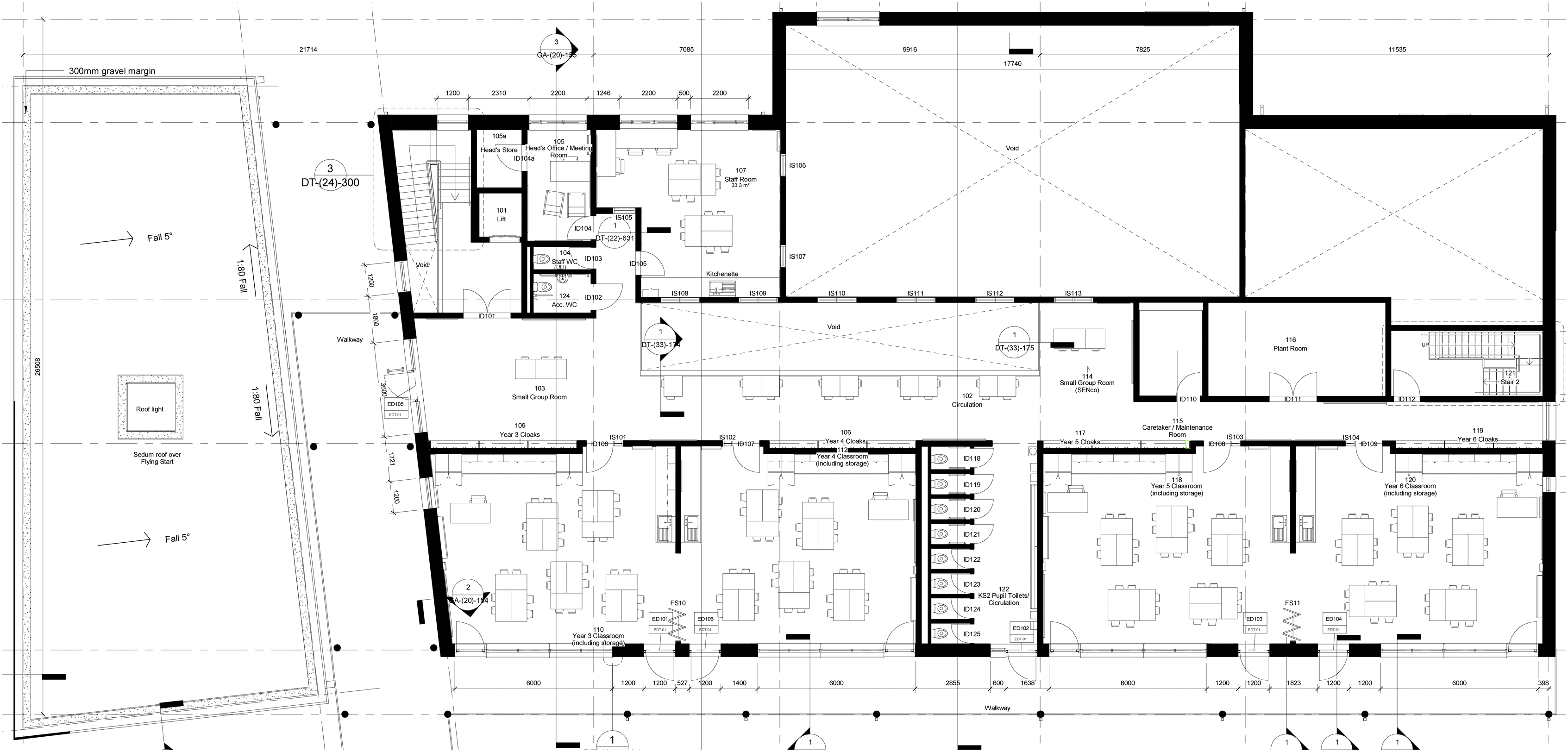
For this case study, the building’s architectural design drawings, such as the typical floor plan presented in Figure 3, are used to inform PHPP inputs sheets, such as:

• Fabric U-values & airtightness: In this sheet construction assemblies for wall, floor and roof fabric elements are defined for use in heat transfer calculations. The building, designed for high energy efficiency, has low U‐values and emphasises avoiding thermal bridging. U‐values (W/m²K) are as follows: Wall: 0.144; Floor: 0.131; Roof: 0.109; and air permeability as 0.64 m³/hr/m² @ 50 Pa. ¹

• Areas: For building assembly (zones, and fabric elements), the total thermal envelope surface area is 3,129 m² and Treated Floor Area (TFA) is 1,327 m². Thermal bridges are defined along with areas in the same sheet in PHPP. The total length of thermal bridges to ambient air (psi: 0.165 W/mK) is 29 m and the length of the perimeter thermal bridge (psi: 0.017 W/mK) is 10 m.

• Ground: Details including soil properties (conductivity: 2.0 W/mK; Heat capacity: 2.0 MJ/m²K) and ground slab details (U‐value: 0.131 W/m²K; area: 374 m²; perimeter: 125 m) are defined for accurate calculation of ground heat transfers.

• Windows and doors: Geometry and frame details for windows (window area: 277 m²; glazing area: 196 m²), orientation (north: 20%; east: 5%; south: 65%; west: 10%) and thermal properties (glazing U-value: 0.6 W/m²K; glazing g-value: 0.5; frame U-value: 0.73 W/m²K; door U-value: 1.4 W/m²K) including thermal bridging of glazing (psi window: 0.04 W/mK; psi door: 0.1 W/mK).

• Shading: Details of shading from building elements (overhangs and reveals) to calculate the shading coefficient for each of the windows along with shading from surrounding buildings.

Figure 3.

First-floor plan of the school.

Climate data for Zone 14-Wales is used from the 22 climate data sets in the UK included within PHPP. This data is generated using ‘Met Office’ data and ratified by the Passivhaus Institute. ⁵ It contains details such as average monthly temperatures (external, dew point, sky, and ground) and radiation levels (horizontal and for each direction).

The confidence level in the construction inputs is considered high due to the building being designed to high Passivhaus standards. Therefore, it is assumed that typical variation in the designed thermal properties will be negligible.

Operation details and internal gains

Building occupancy numbers and thermal loads related to internal casual gains such as lighting and equipment along with the intended hours of operation of the plant and equipment must be established as far as possible. These are typically estimated by assessing the installed equipment and establishing the occupied (or operating hours) of the building and the way the building is to be managed. While design documentation can provide the nominal occupancy and internal loads, an information request (using a form or a structured interview) from the intended occupiers is the best way to establish the operations. In scenarios where this information is not readily available, typical assumptions, representative of the building type, can be used for baseline modelling with a high degree of uncertainty, which should be further explored in scenario and sensitivity analysis.

Occupancy and internal gain data in the case study model are defined based on design stage documents and the users’ feedback for building operations. In the PHPP calculation for this case study, the building loads for internal heat gains are based on a whole building approach and not defined for individual rooms ² . The rest of this section explains these model inputs in detail, covering each of the steps defined in TM54.

Step 2: Estimating operating hours and occupancy factors

Typical building utilisation is from 9 am to 3 pm for areas primarily used for teaching and by the students. Slightly extended 8 am to 5 pm operating hours are defined for offices and circulation spaces. Based on utilisation of 200 days/annum (factoring in school holidays) the total building operating hours for regularly used and extended use spaces are 1200 h and 1800 h respectively. Classrooms and offices are designed to have 100% occupancy during working hours with occupancy densities of 2 m²/person and 5 m²/person respectively. Other rooms are considered transition spaces and therefore considered unoccupied.

Step 3: Lighting

Lighting gains are based on the planned lighting equipment. The building is planned to have daylight-integrated, low-energy lighting with controls including daylight and PIR sensors. Different space types have target lighting levels set as 300 lux for classrooms, halls, circulation, and store areas; 500 lux for offices and the kitchen; and 150 lux for toilets. Lighting power density varies between 4-10 W/m². PHPP has a predefined set of rules to calculate full load hours of lighting depending on the types of sensors used (daylight, PIR etc.). The hours of lighting use per year are between 700-1000 h for all spaces except stores and toilets which are manually set for 200 h.

Step 4: Lifts and escalators

In this building, there is only one lift and to simplify calculations its load is modelled within small power energy us in the next step.

Step 5: Small power

The key energy end-uses in the building, covered in small power, include computers, office equipment, and other plug-in loads. Total loads add up to 4.3 kW load including computers and other displays, equating to about 3 W/m². The total utilisation hours per year are estimated to be 1080 h.

Step 6: Catering

This load is primarily for cooking, refrigerating, and dishwashing. The building is assumed to serve 144 meals per day for a 200-day school year. The normalised energy consumption per meal, as pre-defined in the PHPP spreadsheet , ³ is 0.25 kWh for cooking and 0.1 kWh for dishwashing. Energy demand for fridges is estimated at 14.01 kWh/day for 365 days.

Step 7: Server

The building has a small server room with 1500W capacity operating all year for 8760 hours.

Step 8: Plant and equipment

load from additional plant equipment such as telecom switches, BMS, interactive displays and sprinkler frost protection has been modelled within small power energy use in step 5.

Step 9: Domestic hot water (DHW)

Hot water is used in the toilets and the kitchen. The equivalent average amount of water at 60°C is estimated as 350 L/day. DHW demand is calculated for 240 persons with predefined energy use per person and per area in PHPP spreadsheets. ³ The total useful heat required is calculated as 2.8 kWh/m²/annum.

Additionally, based on class ratings of the DHW tanks, heat loss ratios have been pre-defined in PHPP. For the two DHW storage tanks of 70 L and 30 L, storage and distribution losses have been calculated as 2.2 kWh/m²/annum. Therefore, total DHW energy use is calculated as 5 kWh/m²/annum.

Step 10: Adding internal heat gains to the model, for energy uses calculated outside the model

Data inputs from operations and gains as per TM54 are defined from Steps 2 to Step 8. Following this, Step 10 requires adding internal heat gains to the model, for any energy uses calculated outside the model. The simulation tool used for the quasi-steady stage calculations already includes calculations for the impact of internal gains on the heat balance at the overall building level. There were no additional energy uses that were calculated outside the model.

The confidence level in the occupancy-related factors (Steps 2-9) is low, similar to most buildings at the design stages. Therefore, a typical variation is expected to be seen in these inputs from what is estimated here and in the actual building. These variations can be up to ±10% as per BS EN 15603:2008 ⁶ and have been used to inform the sensitivity analysis.

HVAC system definition

Step 11: Modelling HVAC systems and their controls

The energy use for HVAC systems and associated controls is required to be estimated and separately reported. This energy use should include all HVAC systems including heating and cooling, ventilation fans and pumps.

In Step 11, in this case study, quasi-steady state modelling is used which is based on monthly-averaged heat balance and climatic conditions. This approach for projecting energy use of the HVAC system is appropriate because the systems used in the building are simple with limited interactions with each other and their performance does not vary significantly with slight changes in heat balance expected during routine operation of school buildings or hourly external weather.

Heating in the building is provided by a 45-kW gas boiler (seasonal gross efficiency: 0.95) and radiators with individual thermostatic valves. Mechanical ventilation in the hall, classrooms and other spaces is provided by a main AHU. A separate AHU serves the kitchen.

The heating and ventilation strategy in winter involves demand-controlled heat recovery supply in classrooms. Each classroom is equipped with a CO₂ sensor. Used air transfers to the circulation/hub spaces and is extracted from the circulation roof spaces. In the summer, natural ventilation, via user-operated windows, provides comfort cooling (often coupled with night ventilation) and mechanical ventilation supply is without heat recovery. The heating setpoint is set to be 20°C. The mechanical ventilation rate for the occupied spaces is 1.5 air changes per hour (ach) in regularly occupied spaces and 12 ach in the kitchen. The mechanical ventilation system power density at full load is 0.45 W/m² with a heat recovery efficiency of 81% for the main school AHU and 54% for the one in the catering kitchen.

TM54 baseline results

As the key modelling inputs have been set up by Step 11, TM54 baseline performance projection can be calculated. The building’s energy use is calculated as 41 kWh/m²/annum. Figure 4 shows the breakdown of this projected energy use, separated by end uses.

Figure 4.

TM54 Baseline energy use per end-use for the baseline building.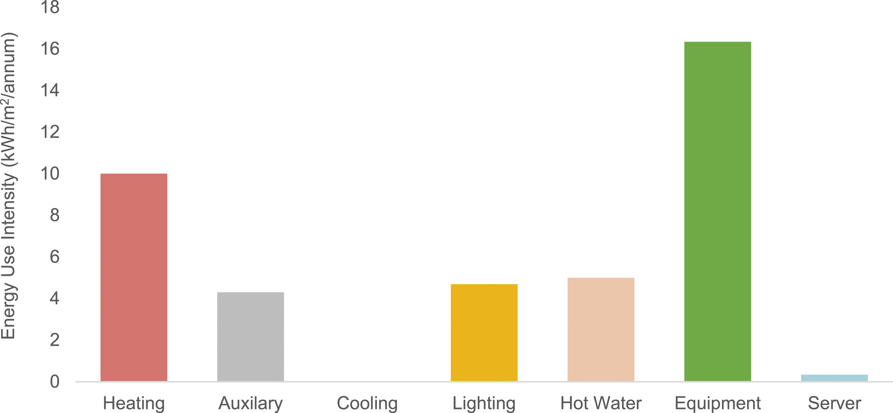

Building energy use, specifically for the heating of the building, is low due to the Passivhaus specifications for the building fabric. The energy used for heating, shown in the graph, is the gas used by the boiler. The rest of the energy end-uses (auxiliary energy for fans and pumps, lighting, domestic hot water, equipment, and the server) are fuelled by electricity. The use of natural ventilation for cooling purposes means there is no cooling energy used.

This is the central or nominal estimate of energy performance. However, for better communication of expected building performance, realistic scenarios that account for uncertainty in modelling assumptions should also be presented.

Scenario/sensitivity analysis

Performance projections at the design stage are prone to several operational risks. These risks can be due to variations in the specification or performance of building systems under real operating conditions, management of the building (Step 12) or functional changes that occur in the building over time. To account for these risks, a range of simulation scenarios should be undertaken. These simulations should consider the variety of plausible potential real-world operating scenarios, focusing on those parameters which are least certain and/or are most influential. This allows quantification of the difference between the nominal (idealised) performance (Figure 4, at the end of Step 11) and how the building is likely to operate in practice. This risk assessment can be done using a systematic approach for sensitivity and scenario analysis which can identify the most important and influential model inputs (Step 13) and quantify the total variability in the calculation results (Step 14). As a part of the TM54 Baseline modelling process (Steps 1–11), all key input parameters were tagged with the confidence level in their values.

For this building, four different scenarios/sensitivity assessments were undertaken to quantify the impact of key uncertain model input parameters on the energy use outputs.

1. Future climate scenario assessment.

2. Differential sensitivity analysis by varying one input variable at a time, within its typical upper and lower limits.

3. Typical high and low energy use when all inputs are changed together within their typical variable limits.

4. Worst case scenario that assumes a poorly managed building with extended running hours, high occupancy, and high levels of internal gain loads.

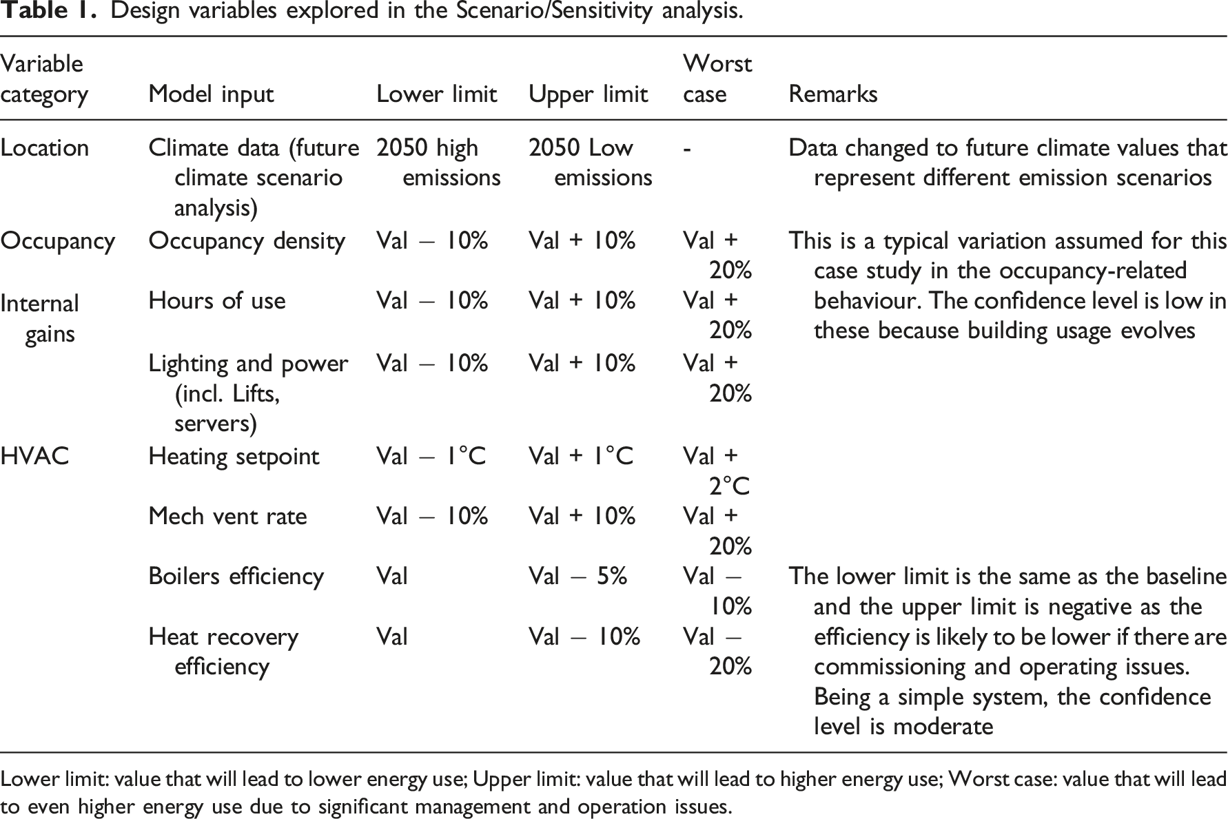
Table 1 lists all the uncertain variable categories, the model inputs that are changed, and their variation (lower limit, upper limit, and worst case) assumed in the sensitivity analysis. The variations are those that are assumed by modellers based on their experience, published literature,^6,7 and stakeholder discussions. Being a Passivhaus design, construction-related uncertainties are expected to be very low. Therefore, it was assumed that the effect of variation in these input parameters on energy performance results would be negligible.

For future climate scenarios assessment, the ambient temperatures are expected to increase, leading to a reduction in the heating energy use of the building. The weather data used ³ for the lower limit was 2050 high emissions compared to the 2050 low emissions scenario being used as the upper limit because in the former the increase in temperature is greater. The results showed only a slight decrease in total energy use in both cases because heating accounts for a lower proportion of total energy. For the lower limit and upper limit, the energy use is 39 kWh/m²/annum and 40 kWh/m²/annum respectively. It should be noted that with increasing temperatures, the building, not having comfort cooling, will see a significant amount of overheating in summer and this may necessitate the installation of a cooling system in the future. Such an analysis can inform design decisions and recommendations for the long-term management of the school.

Figure 5 shows the differential sensitivity analysis of total energy use in the building. Multiple calculations were undertaken making one change at a time for each of the model input categories listed in Table 1. The bar represents the central (nominal) energy use, and the whiskers show the high and low energy use for the variability of that particular input parameter. It can be observed that, within the range of variability assumed, occupancy and occupant behaviour (hours of use, lighting and power density, and heating setpoints) and mechanical ventilation are more influential parameters that affect the total energy use of the building. The occupant-related factors are significantly more important than the external environment due to the school having an extremely thermally efficient and airtight envelope.

Figure 5.

Variation of total energy use due to input variation.

Table 1.

Design variables explored in the Scenario/Sensitivity analysis.

Variable category	Model input	Lower limit	Upper limit	Worst case	Remarks
Location	Climate data (future climate scenario analysis)	2050 high emissions	2050 Low emissions	-	Data changed to future climate values that represent different emission scenarios
Occupancy	Occupancy density	Val − 10%	Val + 10%	Val + 20%	This is a typical variation assumed for this case study in the occupancy-related behaviour. The confidence level is low in these because building usage evolves
	Hours of use	Val − 10%	Val + 10%	Val + 20%
Internal gains
	Lighting and power (incl. Lifts, servers)	Val − 10%	Val + 10%	Val + 20%
HVAC	Heating setpoint	Val − 1°C	Val + 1°C	Val + 2°C
	Mech vent rate	Val − 10%	Val + 10%	Val + 20%
	Boilers efficiency	Val	Val − 5%	Val − 10%	The lower limit is the same as the baseline and the upper limit is negative as the efficiency is likely to be lower if there are commissioning and operating issues. Being a simple system, the confidence level is moderate
	Heat recovery efficiency	Val	Val − 10%	Val − 20%

Lower limit: value that will lead to lower energy use; Upper limit: value that will lead to higher energy use; Worst case: value that will lead to even higher energy use due to significant management and operation issues.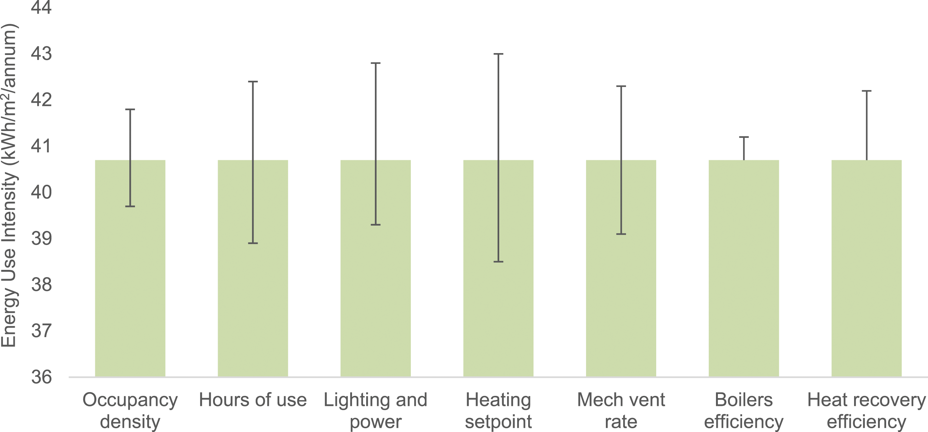

Combining the variations for the input parameters in Table 1, the overall variation (uncertainty) in total energy use output ranges between 33 kWh/m²/annum for the lower limit and 52 kWh/m²/annum for the upper limit. Therefore, if the building is to perform as intended the most influential parameters listed above would require close monitoring and safeguarding from significant changes.

Besides the upper and lower range of likely building performance, the worst-case scenario energy use is also calculated as 68 kWh/m²/annum. This worst-case assumes a poorly managed building with the values under the worst-case column in Table 1.

Reporting and benchmarking

Presenting simulation results in context, comparing them with benchmarks, and building targets can be useful to determine whether the results are within an acceptable range. Figure 6 shows the comparison of TM54 baseline estimates against the good practice (25^th percentile) and typical (median) benchmarks as per the DEC database, ⁸ and CIBSE TM46 benchmarks. ⁹ It is seen that the TM54 central estimate is almost 70% below good practice benchmarks, especially due to very low heating (fossil fuel) energy use. For electricity, the central estimate is also better than the good practice benchmark, however, the uncertainty (seen in Figure 5) and the worst-case performance projection mean that it is possible for the building to exceed this value if safeguards are not put in place to manage electricity use during operations. In either case, however, the total energy use is expected to remain about 50% below benchmark aggregates.

Figure 6.

Simulated energy use compared to industry benchmarks.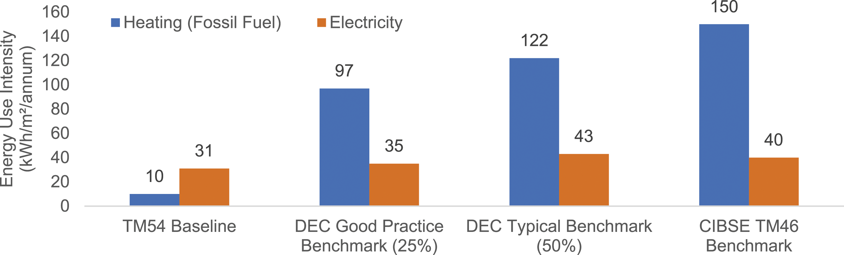

Result reporting for TM54 calculations should not just be limited to central estimates, as seen in Figure 4, but also include further assessments undertaken after scenario/sensitivity analysis along with a comparison against operational benchmarks. Reporting of modelling inputs and outputs in a structured implementation matrix (for an example, see Annex A of CIBSE TM54 ² ) allows for documentation of all the assumptions that have been made alongside the results, at each modelling step. While this keeps the modelling process transparent, it also provides useful documentation for operational stage performance assessments.

Operational performance of the building

This case study is an example application for CIBSE TM54, which focuses on the design stage projection of energy use. These design calculations are based on the best estimates that are available to the modelling team during the design stage. The actual energy use can be very different, even when calculated with best practice modelling at the design stage. Using TM54 performance modelling the compliance gap ² can be eliminated but a performance gap may still occur due to many changes that might happen in a building including those that cannot be estimated at the design stage. The underlying causes of an energy performance gap go beyond the scope of modelling in TM54 and its accuracy. These causes can be mapped to several factors across various construction stages. ¹⁰

The building’s energy use in the second year of operation is metered as 48 kWh/m²/annum. This is slightly higher than the central estimate in ‘TM54 baseline results’ section but within the uncertainty range calculated in ‘scenario/sensitvity analysis’ section. The identification of the root causes of the deviation is beyond the scope of TM54 methodology and this case study document. CIBSE TM63 Operational performance: Modelling for evaluation of energy in use ¹¹ provides a calibration-based modelling framework and a step-by-step guide for measurement and verification of energy performance in use. The framework is designed to determine the energy performance gap in operation concerning design calculations and identify the root causes of the gap. It builds upon the design stage modelling done as per TM54 and is the natural successor of this TM for modelling and diagnosis during post-occupancy evaluation.

Summary

The following key points emerge from the CIBSE TM54 energy projections for this case study school building using a quasi-steady-state modelling approach:

• The school building has a compact design and highly insulated envelope with low air permeability. Additionally, as the building uses rather simple heating and ventilation systems with predictable operational patterns, it can be assumed that building simulation results will not vary significantly with slight changes in heat balance or hourly external weather. These considerations can help determine which TM54 modelling route is the best option for a given context.

• Consequently, a simplified modelling approach can be used in this case. The quasi-steady state building energy modelling approach was used to develop the TM54 model of this building.

• Step-by-step modelling following the TM54 procedures, factoring in all energy end-uses and operational details, resulted in a projection of 41 kWh/m²/annum for the total energy performance of the building. This can be reported as the nominal projection (or central estimate) of operational energy performance if the building specification and operation are consistent with the nominal input data.

• Scenario/Sensitivity analysis shows that the building performance is susceptible to underperformance due to mainly occupant-related factors such as building occupancy, hours of use, internal gains and setpoint temperatures.

• Within reasonable uncertainty of model inputs and operational changes, the total energy use of this case study building can range between 33 kWh/m²/annum and 52 kWh/m²/annum. However, in the case of severe mismanagement and operational issues, it is estimated that this may increase to 68 kWh/m²/annum.