Sage Journals: Discover world-class research

Abstract

CIBSE TM54 was recently revised and covers best practice methods to evaluate the operational energy use of buildings. TM54 is a guidance document on performance evaluation at every stage of the design and construction process, and during the occupied stage, to ensure that long-term operational performance is in line with the design intent. The main performance evaluation principles in TM54 are a step-by-step modelling approach and scenario testing, to improve the robustness of the design proposal calculations. The latest version brings an updated perspective to the modelling approaches, including dynamic simulation with Heating, Ventilation and Air Conditioning (HVAC) systems. It also incorporates more detailed guidance around risks, target setting, scenario testing and sensitivity analysis. A case study approach is used to explore some of the important aspects described in TM54. TM54 recommends three modelling approaches (aka implementation routes) that a project can follow depending on its scale and complexity: using quasi-steady state tools; using dynamic simulation with template HVAC system; and using dynamic simulation with detailed HVAC system modelling. As part of a series of three, this case study provides an application of the second implementation route: using dynamic simulation with template HVAC.

Practical Application

This case study provides detailed guidance on undertaking CIBSE TM54 modelling and projecting design stage building performance. The study covers the interpretation and clarifications of how TM54 can be applied, through the dynamic modelling tools using template HVAC systems.

Keywords

CIBSE TM54 energy performance performance modelling dynamic simulation simple HVAC

Introduction

The Chartered Institution of Building Services Engineers (CIBSE) Technical Memorandum (TM) 54 provides building designers and owners with guidance on evaluating operational energy use once a building’s design has been developed. First published in 2013,¹ this was one of the first pieces of industry guidance documents in the UK to address the performance gap issue and to better project operational performance of actual energy use. In the recently published revision to CIBSE TM54: 2022,² the guidance has been made up to date by taking account of regulatory and industry changes such as net-zero transition, performance targets and advances in Heating, Ventilation and Air Conditioning (HVAC) modelling.

For a holistic application and wider adoption of best practice energy projections in the industry, the new TM54 document suggests three implementation routes for different scales and complexity of projects. The modelling approaches include:

1. Quasi-steady state modelling

2. Dynamic simulation modelling (DSM) using template HVAC systems

3. Dynamic simulation modelling (DSM) using detailed HVAC systems

In this, second of three case studies, an example of TM54 design stage building performance modelling is presented for a school building using dynamic simulation with template HVAC. First, the step-by-step modelling methodology proposed in CIBSE TM54 for this implementation route is described. Then the case study building is introduced and the modelling inputs and assumptions for each TM54 step are described. Finally, results are presented per TM54 requirements including deterministic calculations, sensitivity and scenario assessments, and benchmarking against industry standards.

Methodology

The main performance evaluation principles in TM54 are a step-by-step modelling approach, systematic sensitivity and scenario analysis, and performance reporting including benchmarking, to improve the robustness of the design proposal calculations and provision of advice to clients.

After Step 0, that is, the selection of the appropriate modelling approach, depending on project-specific requirements, step-by-step modelling is undertaken. The modelling approach used in this case study is based on the dynamic simulation method (DSM) with a template HVAC system and its subsequent steps are shown in Figure 1. The 17-step modelling methodology has been divided into three stages: baseline model generation, scenario/sensitivity assessments, and result reporting & benchmarking. In the subsequent sections of the case study, the modelling is presented following the steps presented in Figure 1, explaining the use of building-specific information in creating a TM54 model.

Figure 1.

Step-by-step TM54 methodology for dynamic simulation using template HVAC.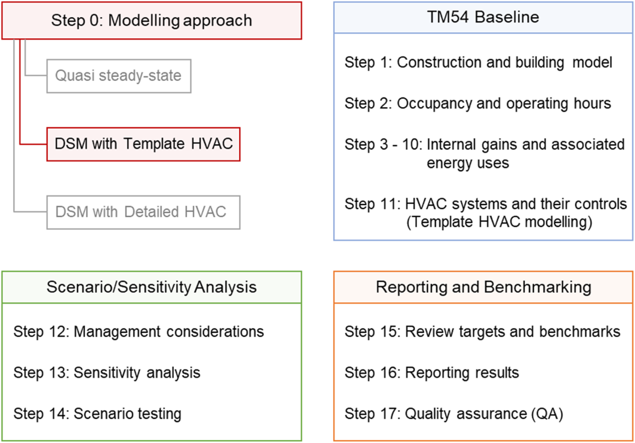

Modelling for TM54 in this case is undertaken using DesignBuilder Software,³ which is a graphical user interface for EnergyPlus.⁴ However, the input definitions and explanations for building details, systems and the project context remain software agnostic. Similarly, results reporting along with process documentation of inclusion or exclusion of any aspects in building modelling also follow TM54 requirements. This makes the case study presentation software agnostic and replicable for any project that uses DSM with a template HVAC modelling approach.

Case study application and modelling approach

The case study building is a secondary school and sixth form with academy status, located in London, England. As part of a redevelopment project, six new buildings have been created for the school, and a couple of existing ones are retained. The buildings are four stories high, with a total useful floor area of 21,405 m². In this case study, we focus on one of the new teaching buildings (∼5000 m²), with typical educational activities such as classrooms, science labs, and faculty rooms. The project is planned to have a biomass boiler using wood pellets and solar thermal collectors to meet the local council’s planning conditions of having on‐site renewable energy technologies.

This school is a large building with complex and varying operation and occupancy patterns, which can be accurately modelled only by using a DSM modelling approach. The HVAC system in the school building, has typical components and simple controls. This means that a high level of detail in HVAC modelling and component-level energy breakdown is not necessary. Therefore, DSM with a template-based HVAC modelling approach is sufficient for this case study. 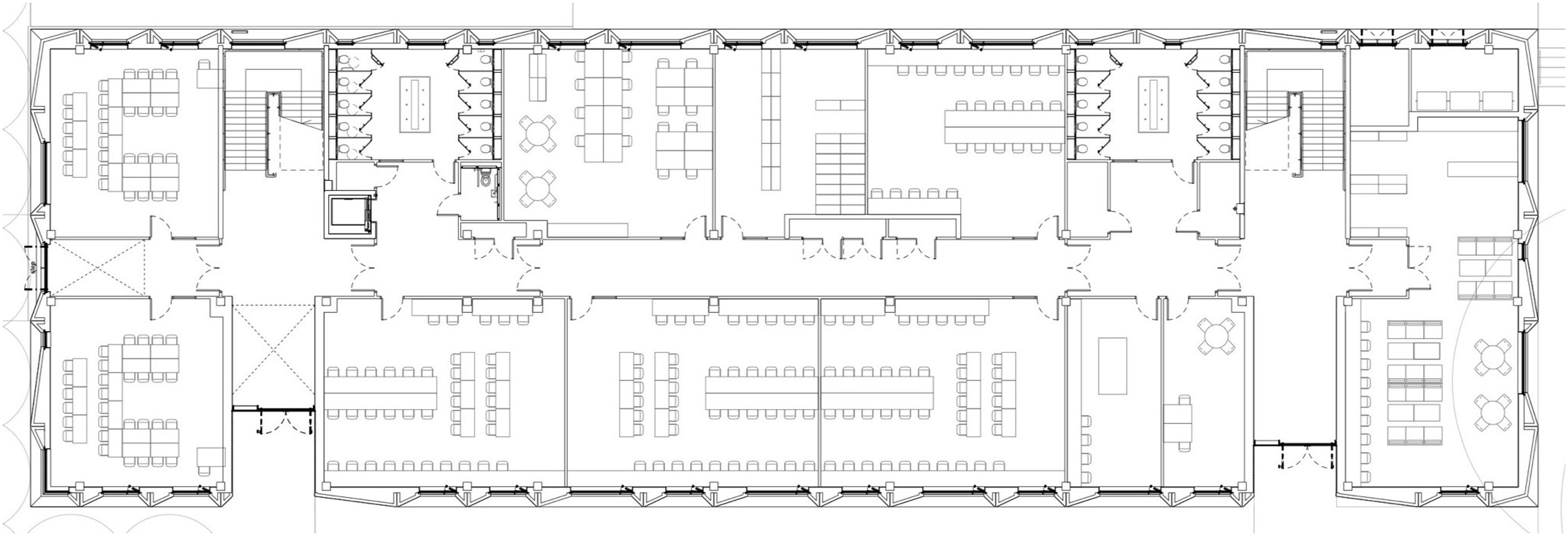Detailed guidance on modelling approaches and tools is explained in TM54.² Figures 2 and 3 show the building’s exterior image and a typical floor plan respectively.

Figure 2.

Case study school building.

Figure 3.

Typical floor plan.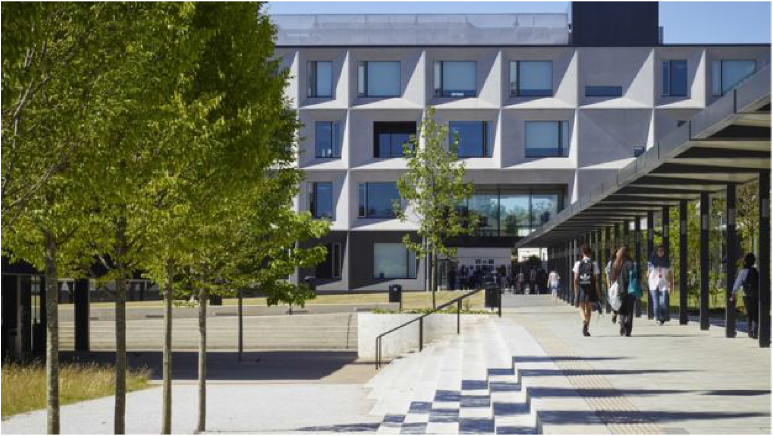

TM54 baseline

The baseline building generation is covered in TM54 Steps 1 – 11. For each of the steps, model inputs must be defined along with ascertaining confidence levels in their assumptions to guide 5.0 Scenario/Sensitivity analysis.

Geometry and site details

Step 1: constructing and building the model

Generating the model geometry and setting up site information is the first step in undertaking building modelling and forms the basis from which all future calculations are undertaken. The process involves creating geometry, defining constructions, zoning, and selecting appropriate weather data. The accuracy and quality of these inputs in the model will in turn affect the accuracy of future model outputs.

For this case study, the building’s architectural design drawings (Figure 3) are used to inform the inputs for geometry, construction, and zoning. Construction details are defined with material layers and typical year-hourly weather data from the nearest weather station is selected for the simulations. Figure 4 shows the model image and internal zoning of the floor plans. In the model, various space types, separated into zones, are teaching areas (60%), circulation (25%), offices for staff (6%), storerooms (3%), high ICT rooms (3%), toilets (2%) and a server room (1%).

Figure 4.

Model visualisation of the school building and its internal zoning.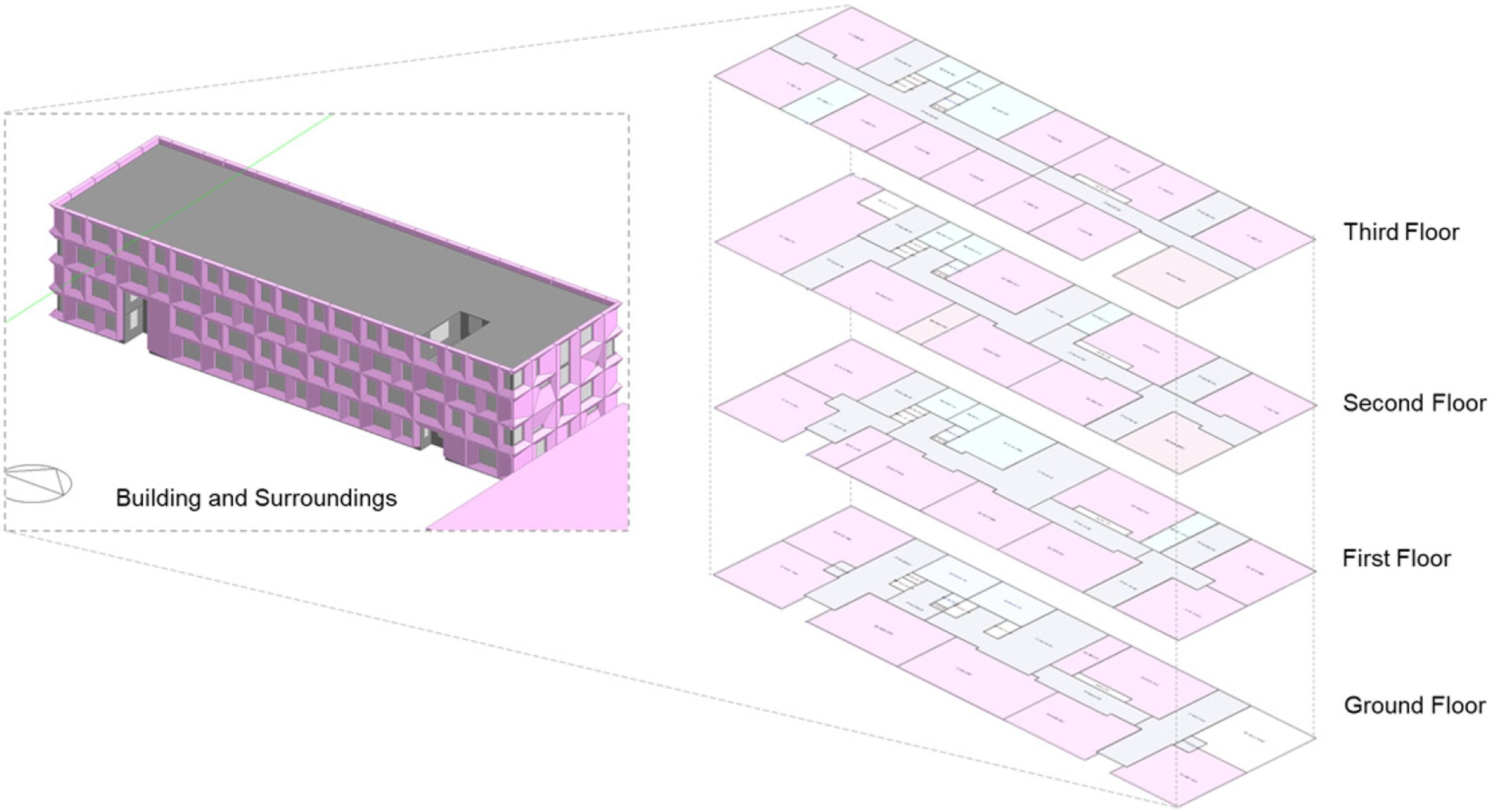

The external envelope is made of prefabricated concrete panels, assembled at the site. The building, designed for high energy efficiency, has low fabric U‐values and emphasises avoiding thermal bridging. Fabric properties are as follows: U‐values (W/m² °K) for Wall: 0.25; Window: 1.6; Roof: 0.20; Ground: 0.15; and design airtightness was 5 m³/hr/m² @ 50 Pa. Glazing has a g-value of 0.26 and visible light transmission (VLT) of 0.49. Appropriate insulation has been added and glazing selection undertaken to meet these values.¹ Spaces are designed to have large windows for daylighting which are also partially operable for natural ventilation and free cooling in summer.

The confidence level in the construction inputs is high due to the use of a prefabricated construction process. Therefore, it is assumed that typical variation in the designed thermal properties will be lower than normal.

Operation details and internal gains

Building occupancy numbers and other loads related to internal gains such as lighting and equipment along with the intended hours of operation of the plant and equipment must be established as far as possible. They are typically estimated by assessing the installed equipment and establishing the operating hours of the building and the way that the building is to be managed. While design documentation can provide the nominal occupancy and internal loads, information gathering from the intended occupiers (for example by conducting a structured interview) is the best way to establish building operation. In scenarios where this information is not readily available, typical building estimates can be used for the baseline modelling with a high degree of uncertainty for scenario and sensitivity analysis.

Data in the case study model about the occupancy and various internal gains are as per the design brief and from discussions with the client for loads and operation. Table 1 summarises the operation details and internal gains for this case study. The rest of the section explains these model inputs in detail, covering each of the steps given in TM54.

Table 1.

Operation details and internal gains for the case study building.

Operation details	Description	Building detail	Remarks
Step 2: Occupancy	This covers gains due to people in the spaces defined by occupancy density and schedules. Indoor environmental quality and operating hours for other loads are often linked to occupancy. They are described in their respective sections.	The whole school campus is designed for 2000 pupils and 250 staff. For building simulation, varied occupancy and schedules are used for different space types. Teaching areas have an average density of 0.42 people/m² with a varying schedule as per the school timetable. Overall occupancy hours for weekdays: 08:30 – 15:00; sun & holidays: nil	Model inputs (density and schedules) for occupancy are set zone-by-zone. This enables the simulation of dynamically varying occupancy-related loads and any ventilation control requirements.
Step 3: Lighting	Lighting energy use and associated heat gains are estimated after defining its loads, operating hours, and controls.	Power density for classrooms, labs and offices is 9 W/m² with operation schedule as per the occupancy. The building has T5 fluorescent lamps, passive infra-red (PIR) and daylight sensors.	Total energy use and associated heat gains for all these types of loads are estimated after defining their power ratings and operating hours. As DSM modelling is granular, inputs for these loads are defined zone-by-zone with hourly varying time schedules. This enables the estimation of their dynamically varying energy use and their effect on space-level heat balance.
Step 5: Small power	This includes plug loads, which can be difficult to estimate, especially when the ultimate occupier is not yet known. Benchmark data can provide helpful estimates at the design stage.	Power density for equipment varies between 10 and 50 W/m² across major spaces. The operation schedule is as per the occupancy.
Step 4: Lifts and escalators Step 6: Catering Step 7: Server Step 8: Plant and equipment	Design stage energy projections must account for all end uses. Buildings may have some or all of these energy end-uses. They have to be added accordingly.	This building has a small proportion of load that could be attributed to these additional loads. These included lifts, IT and lab equipment. These are added to zone-level small power.
Step 9: Domestic hot water (DHW)	Evaluating the energy used to provide DHW requires estimating the amount of water used, schedules, system energy losses, and fuel sources. DHW does not affect the heat balance as such.	This usage varies based on space type and at the design stage, typical benchmarks are used, such as teaching areas’ demand that is set at 5 L/person/day.	Building services in the template HVAC system are modelled using ideal loads. DHW mains and supply temperatures are set as 10°C and 65°C.

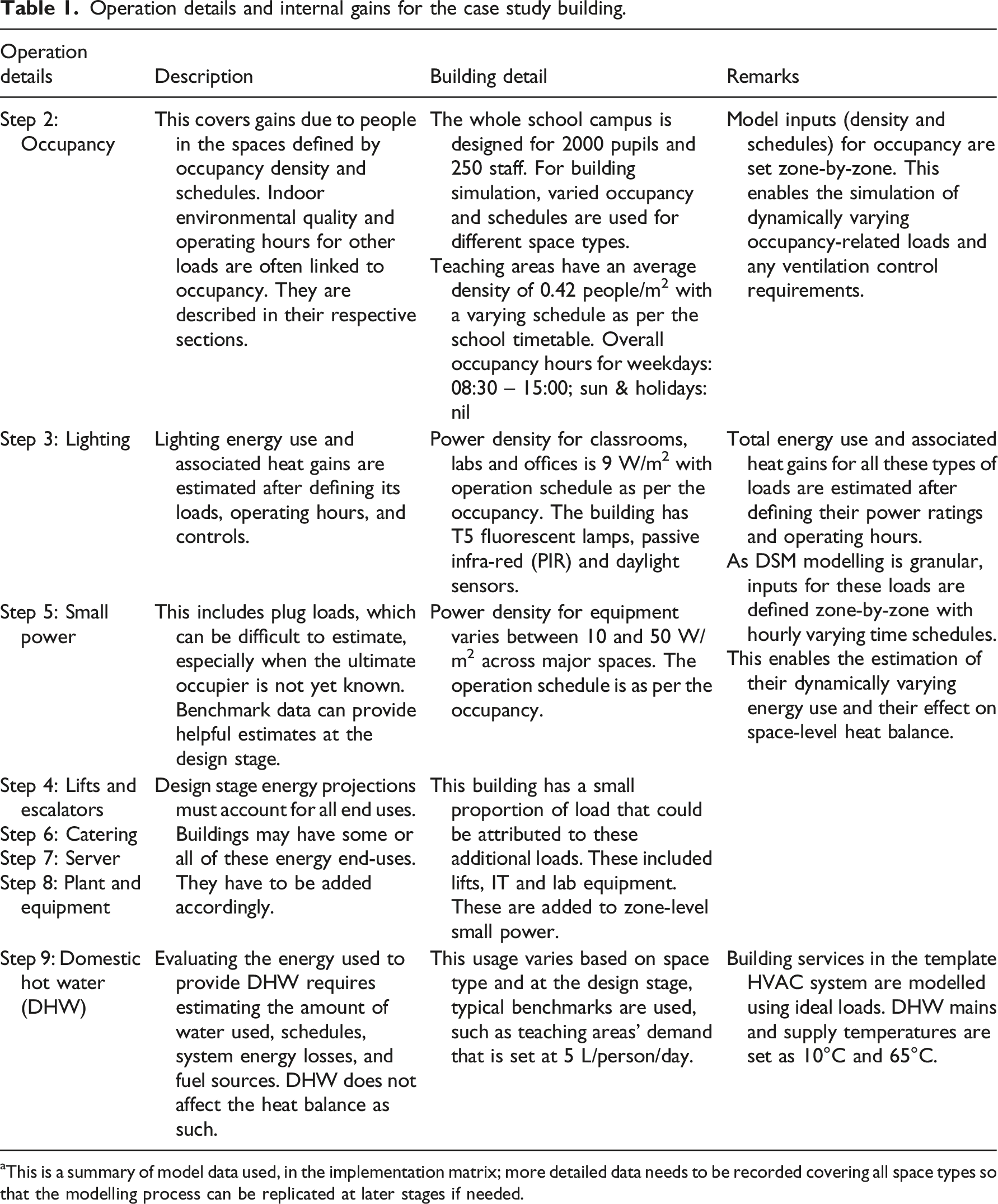
^aThis is a summary of model data used, in the implementation matrix; more detailed data needs to be recorded covering all space types so that the modelling process can be replicated at later stages if needed.

Step 2: estimating operating hours and occupancy factors

Teaching areas, the most common space type, have about 35 persons in the classrooms. The average occupancy density of these areas is therefore 0.42 people/m². Circulation corridors are used between classes and are sparsely occupied. Circulation occupancy density is assumed to be 0.11 people/m² as per UK NCM database.⁵ The other major space type covers office rooms for teaching staff which are occupied by 4–5 staff resulting in an occupancy density of 0.10 people/m². For these three major space types, the occupancy schedules used are shown in Figure 5.

Figure 5.

Occupancy schedules for the school building’s typical spaces.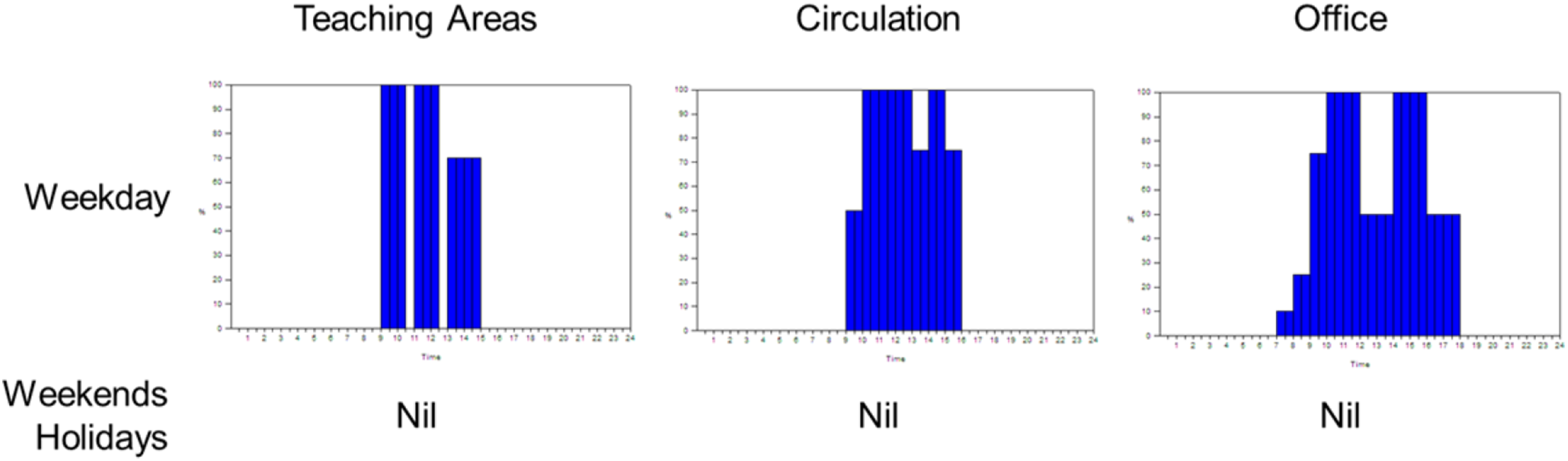

Step 3: lighting

Lighting gains are based on planned lighting equipment. The building is planned to have low-energy lighting (T5 fluorescent lamps) with an efficacy of at least 80 lm/W for teaching areas and offices and 65 lm/W for toilets and circulation areas. Different space types have target lighting levels set as 300–500 lux for teaching areas and 150–200 lux for circulation areas. These are combined with Passive infrared (PIR) and daylight sensors. Lighting power density is set to be 9 W/m² as the building level average and its operation follows the occupancy schedule for each of the spaces.

Step 4: lifts and escalators

In this building, there is only one lift and therefore to simplify its calculations, it is modelled as small power energy use in circulation areas.

Step 5: small power

The key plug-in energy end-uses in the building, covered in small power, include computers, office equipment, lifts, and other plug-in loads. Small power use is assumed to follow the same schedule as occupancy with 5% standby loads. Total loads are defined as follows:

• 1100 W per Teaching Area (or 13.75 W/m² based on 80 m² classroom/lab)

• 50 W/m² in ICT-rich areas

• 10 W/m² for office areas

• 2-10 W/m² in circulation and toilets

Step 6: catering

This load is not represented in this building, as there is a separate building for catering and dining in this school.

Step 7: server

The building server room’s planned capacity is set to be 25 kW which equates to 1000 W/m². Its operation is set to be at full capacity during occupied hours and at 10% standby capacity during non-occupied hours.

Step 8: plant and equipment

The building does not have any significant additional equipment. The security system and any other plug loads are already added in step 5: small power section.

Step 9: domestic hot water (DHW)

The use of hot water is predominantly in the toilets. The typical consumption of hot water is estimated as 5 L/pupil/day as per CIBSE Guide G⁶ reference value for schools.

Step 10: adding internal heat gains to the model, for energy uses calculated outside the model

Table 1 covers all the model data inputs from operations and gains as per TM54 Steps 2 to Step 9. Following this, Step 10 requires adding internal heat gains to the model, for energy uses calculated outside the model. As the modelling process is undertaken using a DSM tool, the impact of internal gains on the heat balance is already included in the calculations. There were no additional energy uses that were calculated outside the model.

The confidence level in the occupancy-related factors (Steps 2–9) is low, similar to most buildings at the design stages. Therefore, a typical variation is expected to be seen in these inputs from what is estimated here and in the actual building. These variations can typically be up to ±10% as per BS EN 15603:2008⁷ and have been used to inform the sensitivity analysis.

HVAC system definition

Step 11: modelling HVAC systems and their controls

The energy use for HVAC systems and associated controls are required to be estimated and separately reported. This energy use should include all HVAC systems including heating and cooling, fans and pumps, and domestic hot water (unless calculated outside the model).

In Step 11, template HVAC modelling is selected, and key model inputs are customised such as equipment coefficient of performance (CoP), whereas other more detailed inputs such as part load performance and controls configuration are assumed to have typical behaviour.

In this case study, a simple HVAC system is proposed. Heating is to be provided through a centralized plant for the entire campus via a pressurised low-temperature hot water (LTHW) system. A biomass boiler (heating seasonal efficiency: 0.75) will provide heat for annual DHW demand and two gas-fired boilers (heating seasonal efficiency: 0.84) will provide the remaining heat and function as a backup to the biomass boiler. ICT-enhanced spaces will have Variable Refrigerant Flow (VRF) systems that provide both heating and cooling in labs and cooling in the server room. (heating/cooling seasonal efficiency: 1.47/3.80). A mechanical ventilation system with heat recovery (efficiency: 0.75) via a centralised roof‐mounted AHU will provide fresh air in the building, distributed through wall‐mounted diffusers/grills. BMS‐control, based on CO₂ sensors will also be used to provide the appropriate amount of fresh air.

Building services operations are linked to occupancy patterns. Space conditioning systems are planned to be turned on 2 h before classrooms are to be occupied until the end of the classes. The heating setpoint is set to be 20°C and in spaces where cooling is provided, the cooling setpoint is set to 23°C. The mechanical ventilation rate for the key occupied spaces varies from 5 to 12 L/s/person with specific fan power calculated as 1.8 W/l/s.

Modelling of this system in this implementation route is carried out by using the Simple HVAC modelling route in DesignBuilder. In ‘Simple HVAC’ the heating/cooling system is simulated using the basic EnergyPlus ZoneHVAC:IdealLoadsAirSystem method.⁸ This supplies hot/cold air to meet heating and cooling loads. Mechanical ventilation loads are also calculated locally for each zone. Subsequently, fuel energy consumption for the boiler and VRF system is calculated from zone heating and cooling loads as a post-process calculation using simple seasonal efficiency factors.

TM54 baseline results

As the key modelling inputs have been set up by Step 11, a simulation for the TM54 baseline performance projection can be run. The building’s energy use projection is 161 kWh/m²/annum. Figure 6 shows the breakdown of projected energy uses, separated by end-use categories.

Figure 6.

TM54 baseline energy use per end use for the baseline building.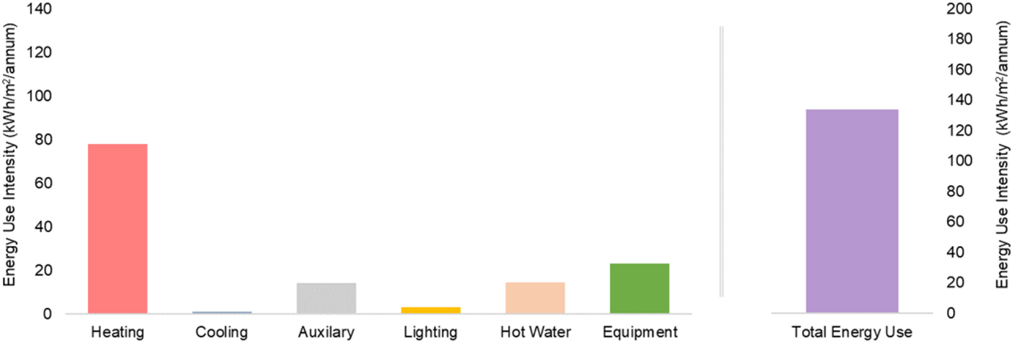

Heating is supplied by the central (biomass and gas) boilers at the facility level and the building level the reported energy use is for this building only, presented as energy use based on the central system’s CoP. Space heating, hot water and CO₂-based demand control ventilation systems (auxiliary energy) account for a major proportion of energy use for the building. This is the central estimate for energy performance. However, for better communication of expected building performance, realistic scenarios that account for uncertainty in modelling assumptions should also be presented.

Scenario/sensitivity analysis

Performance projections at the design stage are prone to several operational risks. These risks can be due to management of the building after occupancy (Step 12) or functional changes that occur in the building over time. To account for these risks, when projecting energy use, a range of simulation runs should be undertaken. These runs should consider the variety of plausible potential real-world operating scenarios, focusing on those parameters which are least certain and/or are most influential. This allows quantification of the difference between nominal performance (Figure 6, at the end of Step 11) and how the building is likely to operate. This risk assessment can be done using a systematic approach of sensitivity (Step 13) and scenario analysis (Step 14) which can identify the most important and influential model inputs and quantify the total variability in the calculation results.

As a part of the TM54 baseline modelling process (Steps 1–11), all key input parameters were tagged with the confidence level in their values. For this building, the impact of key model input parameters which are uncertain such as occupancy and internal gains or which can significantly influence building performance such as construction quality or weather data are explored in the sensitivity analysis. Table 2 lists all the uncertain variable categories, the model inputs that are changed, and their variation (lower limit, upper limit, and worst case) assumed in the sensitivity analysis. The variations are those that are assumed by modellers based on their experience, published literature,^7,9 and discussions with key stakeholders and building users. Parametric simulations run by changing multiple parameters are undertaken to ascertain the most important design inputs that cause variation in building performance from the central (TM54 baseline) estimate.

Table 2.

Design variables explored in the sensitivity analysis.

Variable category	Model input	Lower limit	Upper limit	Worst case	Remarks
Geometry	Wall U‐values	Val −5%	Val +5%	Val +10%	Despite the use of prefabricated panels, insulation was applied on site, therefore variation due to construction quality issues is possible.
	Window U-value	Val −5%	Val +5%	Val +10%
	Roof U-value	Val −5%	Val +5%	Val +10%
Occupancy	Occupancy density	Val −10%	Val +10%	Val +20%	This is a typical variation seen in occupant-related behaviour. Confidence is low in these variables because typical school usage evolves.
Internal gains	Equipment power density	Val −10%	Val +10%	Val +20%
Internal gains	Lighting power density	Val −10%	Val +10%	Val +20%
DHW	DHW demand	Val −20%	Val +20%	Val +25%
HVAC	Heating setpoint	Val −1°C	Val +1°C	Val +2°C
	Cooling setpoint	Val +1°C	Val −1°C	Val −2°C
	Boilers efficiency	Val	Val −5%	Val −10%	Variation is possible due to commissioning and operation issues. The confidence level is moderate as the HVAC strategy is simple.
	VRF efficiency	Val	Val −5%	Val −10%
	Specific fan power	Val −10%	Val +10%	Val +20%

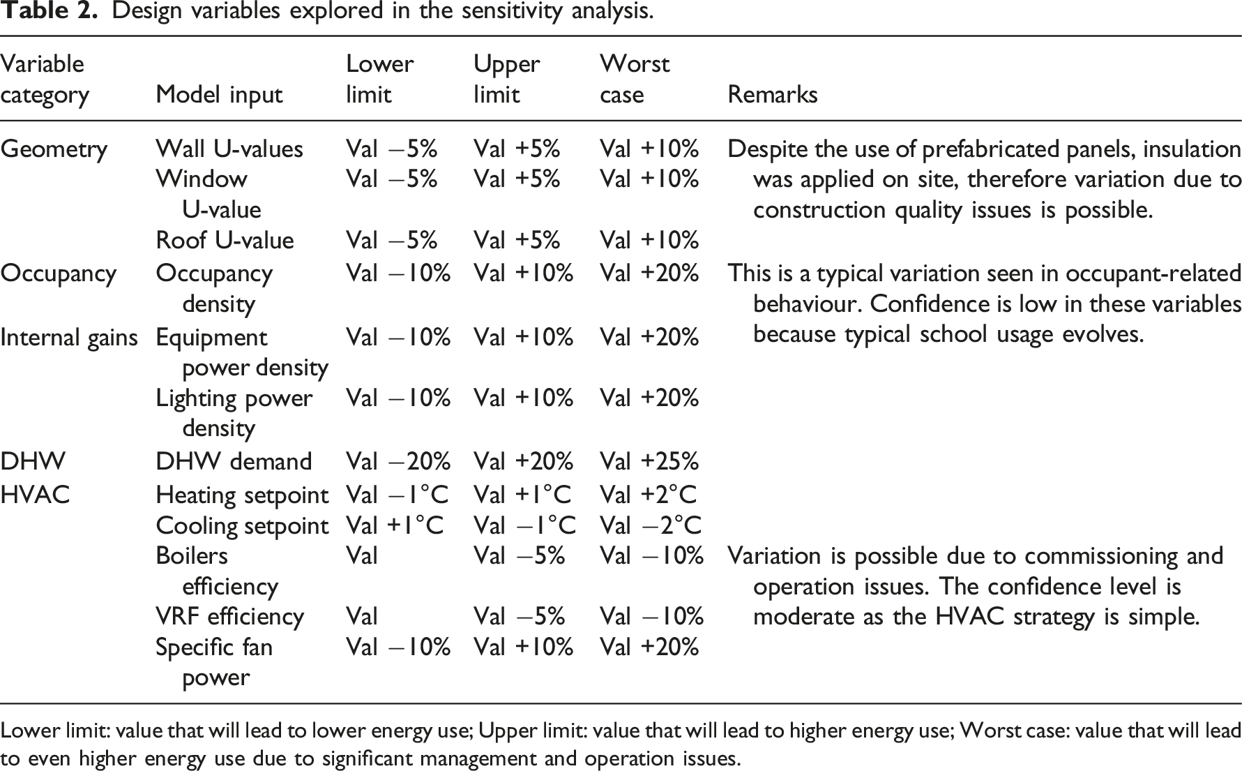
Lower limit: value that will lead to lower energy use; Upper limit: value that will lead to higher energy use; Worst case: value that will lead to even higher energy use due to significant management and operation issues.

Regression-based parametric sensitivity analysis was undertaken by running 250 simulations and changing multiple variables at a time. This analysis assumes that design variables are independent of each other. Figure 7 shows the sensitivity analysis results for total building energy use, ranking the parameters from highest to lowest importance.

Figure 7.

Sensitivity analysis of variable inputs on total energy use.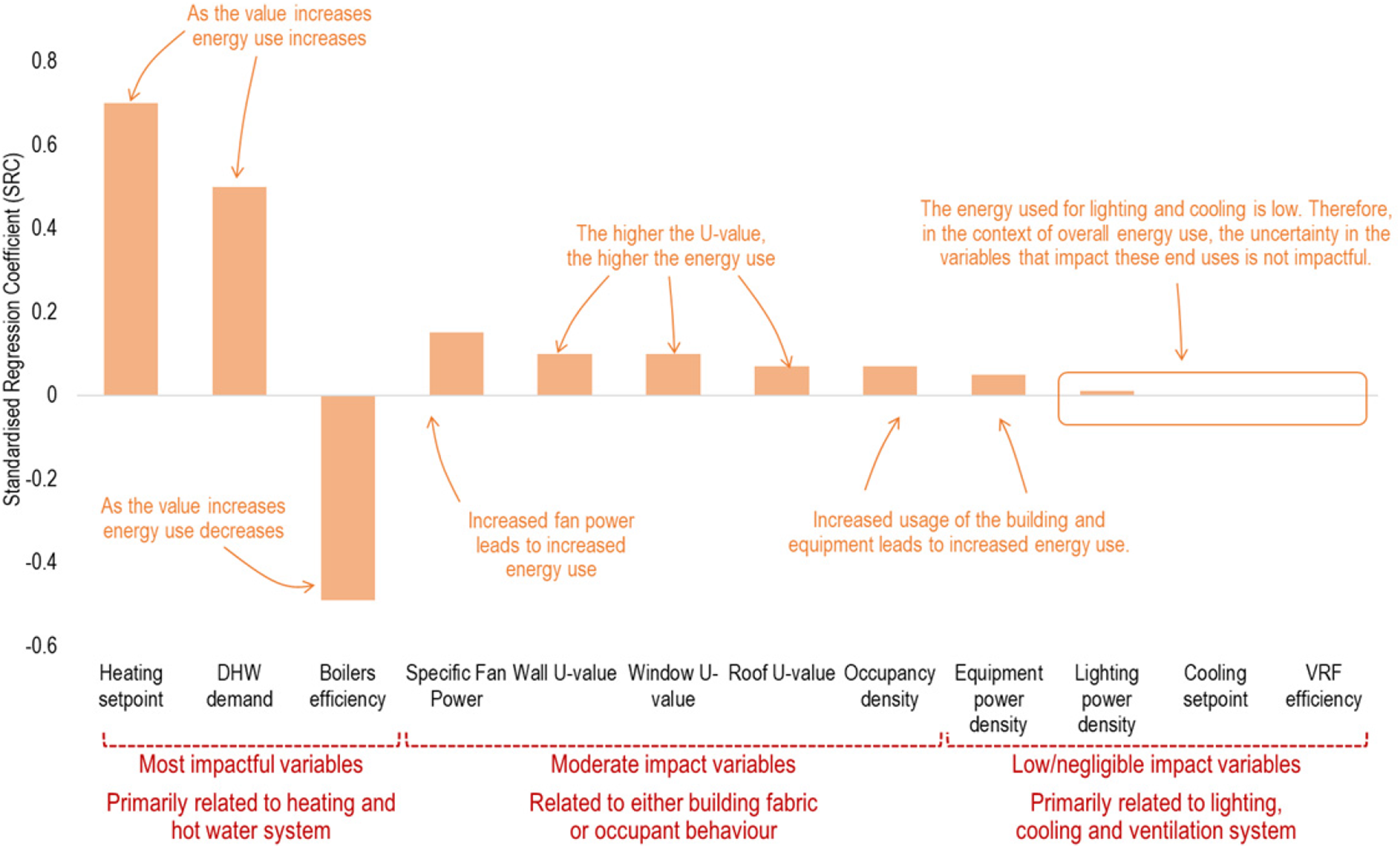

The variables with the highest standardised regression coefficient (SRC) are the most important. For example, within the range of variations assumed, the most influential parameters are heating setpoint, system efficiency, and fabric u-values. All these parameters affect the largest energy end-use (heating energy) significantly and therefore rank highly in the impact on total energy use. The direction of the SRC shows a direct or inverse relationship. For example, if the heating setpoint increases, the total energy use will increase, however, if boiler efficiency increases the overall energy use decreases. Besides these DHW demand is also a highly influential design variable on total energy use.

Uncertainty is also calculated by varying all the input parameters in Table 2 within the ranges defined, the same set of simulations used in the sensitivity analysis above. Figure 8 shows the impact of variability (uncertainty) of all these inputs on individual end-uses and the total energy use. The total energy use of this case study building can range between 113 kWh/m²/annum and 180 kWh/m²/annum. Therefore, if the building is to perform as intended the most influential parameters discussed above would require close monitoring and safeguarding from significant changes.

Figure 8.

Uncertainty around TM54 baseline energy use for various end uses.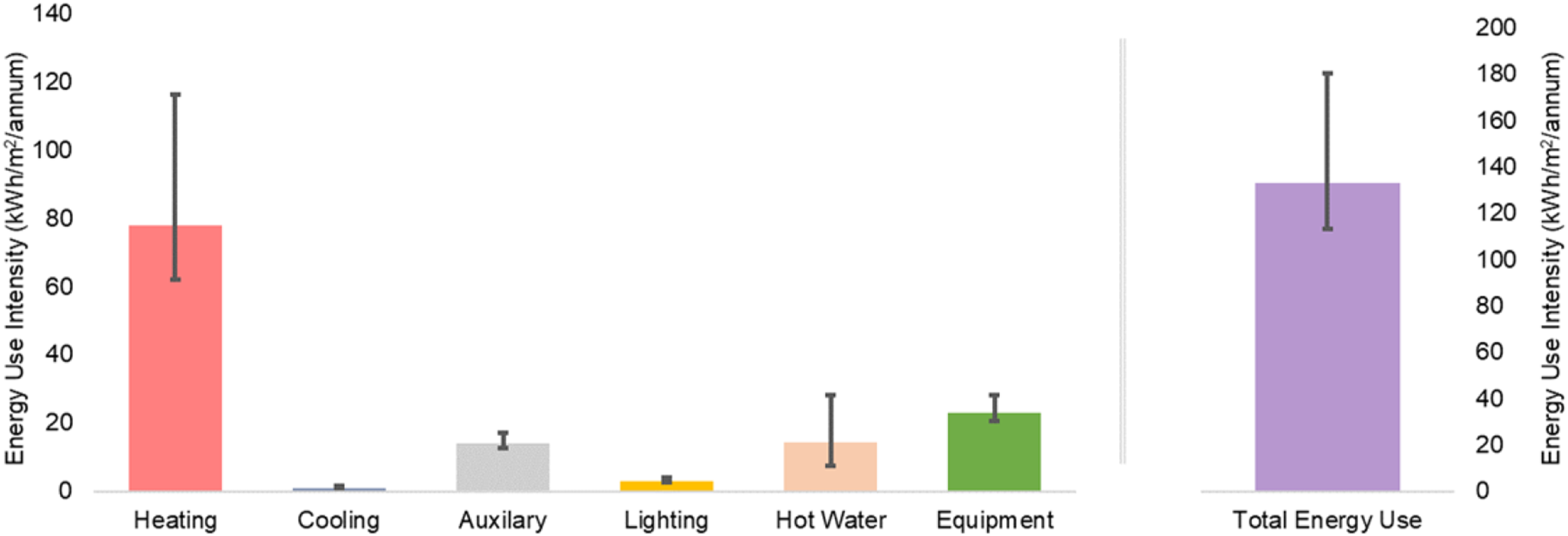

Besides the sensitivity and uncertainty analysis, two distinct scenario analyses were also undertaken:

1. Future climate scenario,

2. Worst-case scenario.

For future climate scenarios assessment, the ambient temperatures are expected to increase, leading to a reduction in the heating energy use of the building. Future climate scenario test is undertaken using 2050 weather data for high, medium, and low emission scenarios² and the total energy use projection is 93 kWh/m²/annum, 102 kWh/m²/annum and 114 kWh/m²/annum respectively. It should be noted that with increasing temperatures the building, not having comfort cooling for most of the spaces, may experience overheating in summer and this may necessitate the installation of a cooling system. Such an analysis can inform design decisions and recommendations for the long-term management of the school.

Besides the upper and lower range of likely building performance, the worst-case scenario energy use is also calculated as 194 kWh/m²/annum. This worst-case assumes a poorly managed building with the values under the worst-case column in Table 2 such as extended running hours, high occupancy, and high levels of internal loads. The current worst case is significantly higher than the central energy use projection and highlights the significance of managing the performance in use.

Reporting and benchmarking

Presenting simulation results in context and comparing them against benchmarks and building targets can be useful to determine whether the results are within an acceptable range. Figure 9 shows the comparison of TM54 baseline estimates against the good practice (25th percentile) and typical (median) benchmarks as per the DEC database,^10,11 and CIBSE TM46 benchmark.¹²

Figure 9.

Simulated energy use compared to industry benchmarks.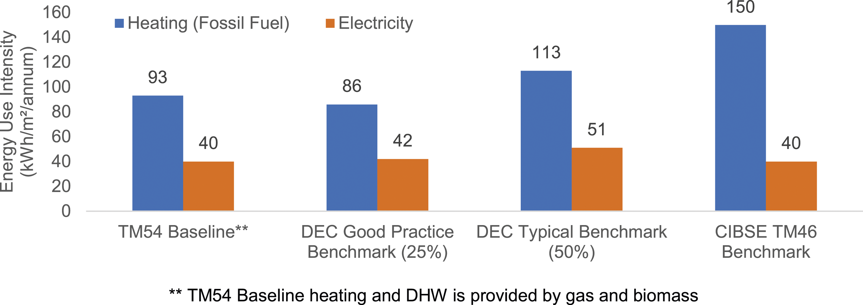

It is seen that the TM54 central estimate is below typical benchmarks. However, the uncertainty (seen in Figure 8) and the worst-case performance projection mean that it is possible for the building to exceed the performance benchmarks if safeguards are not put in place to manage energy use during operation.

Result reporting for TM54 calculations should not just be limited to central estimates, as seen in Figure 6, but also include further results and assessments undertaken after uncertainty and sensitivity analysis along with a comparison against benchmarks. Reporting of modelling inputs and outputs in a structured implementation matrix (Annex A of CIBSE TM54²) allows for documentation of all the assumptions that have been made alongside the results, at each modelling step. While this keeps the modelling process transparent, it also provides useful documentation for operational stage performance assessments.

Operational performance of the building

This case study is an example application for CIBSE TM54, which focuses on the design stage projection of energy use. These design calculations are based on the best estimates that are available to the modelling team during the design stage. The actual energy use can be very different, even when calculated with best practice modelling at the design stage. Using TM54 performance modelling the compliance gap² can be eliminated but a performance gap may still occur due to many changes that might happen in a building including those that cannot be estimated at the design stage. The underlying causes of an energy performance gap go beyond the scope of modelling in TM54 and its accuracy. These causes can be mapped to several factors across various construction stages.¹³

The building’s energy use is metered as 230 kWh/m²/annum. This is higher than the central estimate in ‘TM54 baseline results’ section and also outside the uncertainty range calculated in ‘scenario/sensitvity analysis’ section. The identification of the root causes of the deviation is beyond the scope of TM54 methodology and this case study document. These causes have been determined using CIBSE TM63 methodology¹⁴ and described in a separate paper.¹⁵ CIBSE TM63 Operational performance: Modelling for evaluation of energy in use¹⁴ provides a calibration-based modelling framework and a step-by-step guide for measurement and verification of energy performance in use. The framework is designed to determine the energy performance gap in operation concerning design calculations and identify the root causes of the gap. It builds upon the design stage modelling done as per TM54 and is the natural successor of this TM for modelling and diagnosis during post-occupancy evaluation.

Summary

The following are the key points emerging from the CIBSE TM54 energy projections for this case study school building using dynamic simulation with template HVAC:

• Performance assessment of this school, a large building with varying operational patterns but a rather simple HVAC strategy, was undertaken using dynamic simulation modelling and a template-based HVAC system approach.

• Step-by-step modelling as per TM54, factoring in all energy end-uses and operational details, resulted in an energy use projection of 161 kWh/m²/annum.

• Within reasonable uncertainty of model inputs and operational changes, the total energy use of this case study building can range between 141 kWh/m²/annum and 180 kWh/m²/annum. However, in case of severe mismanagement and operational issues, this can increase to 212 kWh/m²/annum.

• Sensitivity tests show that the building performance is highly susceptible to underperformance due to climate change and uncertainties in building operation. This type of assessment is necessary to have a better understanding of the operational risks and potential mitigation measures that could be considered at design stages and throughout the life cycle of a building.

Footnotes

Acknowledgements

The authors wish to express their gratitude to the designers, building managers and users who engaged in research and supported the building performance evaluation. We specially acknowledge the continued support of AHMM architects, the company which was responsible for the building’s architecture. Photographs in were taken by Tim Soar.

Declaration of conflicting interests

The author(s) declared no potential conflicts of interest with respect to the research, authorship, and/or publication of this article.

Funding

The author(s) received no financial support for the research, authorship, and/or publication of this article.

ORCID iD

Nishesh Jain

Notes

References

CIBSE . TM54: evaluating operational energy performance of buildings at the design stage. London, UK: The Chartered Institution of Building Services Engineers (CIBSE), 2013.

CIBSE . TM54 evaluating operational energy use at the design stage. London, UK: The Chartered Institution of Building Services Engineers (CIBSE), 2022.

DesignBuillder Software Ltd . DesignBuilder V7. Stroud, UK: DesignBuillder Software Ltd., 2023.

NREL . EnergyPlus V9.4. Golden, CO: National Renewable Energy Laboratory, 2021.

BRE . UK NaUK’s national calculation method for non domestic buildings. [Online]. Watford, UK: BRE, https://www.uk-ncm.org.uk/ (2022, accessed 19 12 2023).

CIBSE , Public health engineering CIBSE guide G, London, UK: The Chartered Institution of Building Services Engineers, 2014.

BSI . BS EN 15603:2008 energy performance of buildings. Overall energy use and definition of energy ratings. London, UK: British Standards Institution, 2008.

EnergyPlus Development Team . Ideal loads air system - engineering reference — energyplus 9.4. [Online], https://bigladdersoftware.com/epx/docs/9-4/engineering-reference/ideal-loads-air-system.html#ideal-loads-air-system (2020, accessed 31 May 2023).

Macdonald

. Quantifying the effects of uncertainty in building simulation. PhD thesis, University of Strathclyde, Department of Mechanical Engineering, Glasgow, UK, 2002.

10.

Godoy-Shimizu

Armitage

Steemers

, et al. Using display energy certificates to quantify schools’ energy consumption. Build Res Inf 2011; 39(6): 535–552.

11.

CIBSE . Energy benchmarking dashboard. [Online]. London, UK: CIBSE, 2023, https://www.cibse.org/knowledge-research/knowledge-resources/knowledge-toolbox/energy-benchmarking-dashboard

12.

CIBSE . TM46: energy benchmarks. London, UK: CIBSE, 2008.

13.

CIBSE . Operational performance of buildings CIBSE TM61. London, UK: Chartered Institution of Building Services Engineers, 2020.

14.

CIBSE . Operational performance: building performance modelling and calibration for evaluation of energy in-use CIBSE TM63. London, UK: Chartered Institution of Building Services Engineers, 2020.

15.

Jain

Burman

Stamp

, et al. Cross-sectoral assessment of the performance gap using calibrated building energy performance simulation. Energy Build 2020; 224: 110271.