CIBSE TM54 energy projections III: A case study using dynamic simulation with detailed system modelling

Abstract

CIBSE TM54 was recently revised and covers best practice methods to evaluate the operational energy use of buildings. TM54 is a guidance document on performance evaluation at every stage of the design and construction process, and during the occupied stage, to ensure that long-term operational performance is in line with the design intent. The main performance evaluation principles in TM54 are a step-by-step modelling approach and scenario testing, to improve the robustness of the design proposal calculations. The latest version brings an updated perspective to the modelling approaches, including dynamic simulation with Heating, Ventilation and Air Conditioning (HVAC) systems. It also incorporates more detailed guidance around risks, target setting, scenario testing and sensitivity analysis. A case study approach is used to explore some of the important aspects described in TM54. TM54 recommends three modelling approaches (aka implementation routes) that a project can follow depending on its scale and complexity: using quasi-steady state tools; using dynamic simulation with a template HVAC system; and using dynamic simulation with detailed HVAC system modelling. As part of a series of three, this case study provides an application of the third implementation route: dynamic simulation using detailed HVAC modelling.

Introduction

The Chartered Institution of Building Services Engineers (CIBSE) Technical Memorandum (TM) 54 provides building designers and owners with guidance on evaluating operational energy use once a building’s design has been developed. First published in 2013, ¹ this was one of the first pieces of industry guidance documents in the UK to address the performance gap issue and to better project operational performance of actual energy use. In the recently published revision to CIBSE TM54: 2022, ² the guidance has been made up to date by taking account of regulatory and industry changes such as net-zero transition, performance targets and advances in Heating, Ventilation and Air Conditioning (HVAC) modelling.

For a holistic application and wider adoption of best practice energy projections in the industry, the new TM54 document suggests three implementation routes for different scales and complexity of projects. The modelling approaches include:

(1) Quasi-steady state modelling

(2) Dynamic simulation modelling (DSM) using template HVAC systems

(3) Dynamic simulation modelling (DSM) using detailed HVAC systems

In this, third of three case studies, an example of TM54 design stage energy performance modelling is presented for an office building using dynamic simulation with detailed HVAC modelling. First, the step-by-step modelling methodology proposed in CIBSE TM54 for this implementation route is described. Then the case study building is introduced and the modelling inputs and assumptions for each TM54 step are described. Finally, the results are presented as per TM54 requirements including deterministic calculations, sensitivity and scenario assessments, and benchmarking against industry standards.

Methodology

The main performance evaluation principles in TM54 are a step-by-step modelling approach, systematic sensitivity and scenario analysis, and performance reporting including benchmarking, to improve the design proposal calculations’ robustness and provide advice to clients.

After Step 0, that is, the selection of the appropriate modelling approach, depending on project-specific requirements, step-by-step modelling is undertaken. The modelling approach used in this case study is based on the dynamic simulation method (DSM) with a detailed HVAC system and its subsequent steps are shown in Figure 1. The 17-step modelling methodology has been divided into three stages, baseline model generation, scenario/sensitivity assessments and result reporting & benchmarking. In the subsequent sections of the case study, the modelling is presented by following the steps presented in Figure 1, explaining the use of building-specific information in creating a TM54 model.

Figure 1.

Step-by-step TM54 methodology for dynamic simulation using Detailed HVAC.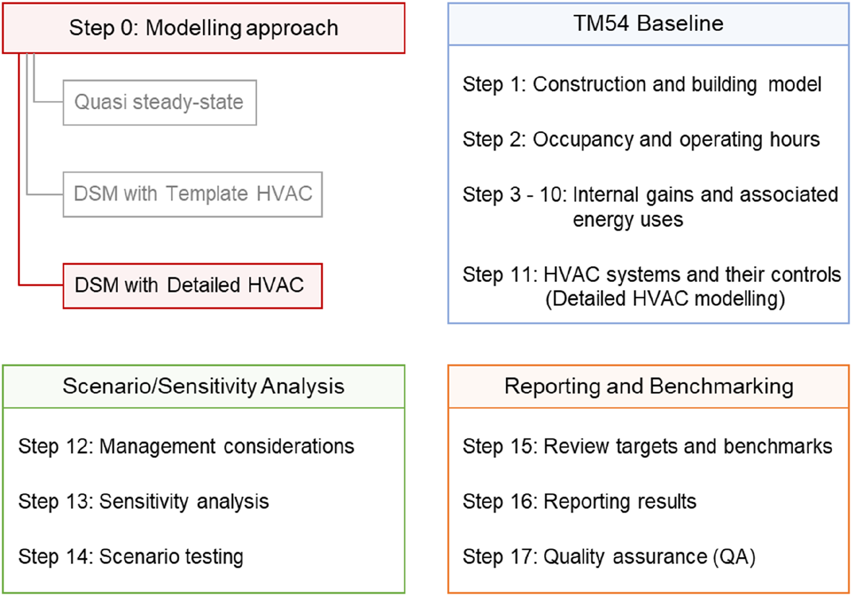

Modelling for TM54 in this case is undertaken using DesignBuilder Software, ³ which is a graphical user interface for EnergyPlus. ⁴ However, the input definitions and explanations for building details, systems and the project context remain software agnostic. Similarly, results reporting along with process documentation of inclusion or exclusion of any aspects in building modelling are also as per TM54 requirements. This makes the case study presentation software agnostic and is replicable for any project that uses DSM with a template HVAC modelling approach.

Case study application and modelling approach

The four‐storey office building is approximately 6500 m² and is located in Keynsham in Southwest England. It is a new building designed primarily to house open‐plan offices with meeting rooms. The building is highly insulated, and the architectural design promotes passive design. The building has a design target to achieve the highest UK rating of DEC-A ¹ by the second year of operation. To ensure this, the project team are responsible for the operational performance of the building, which is embedded in an energy performance contract. Figure 2 shows the building’s exterior image.

Figure 2.

Case study office building.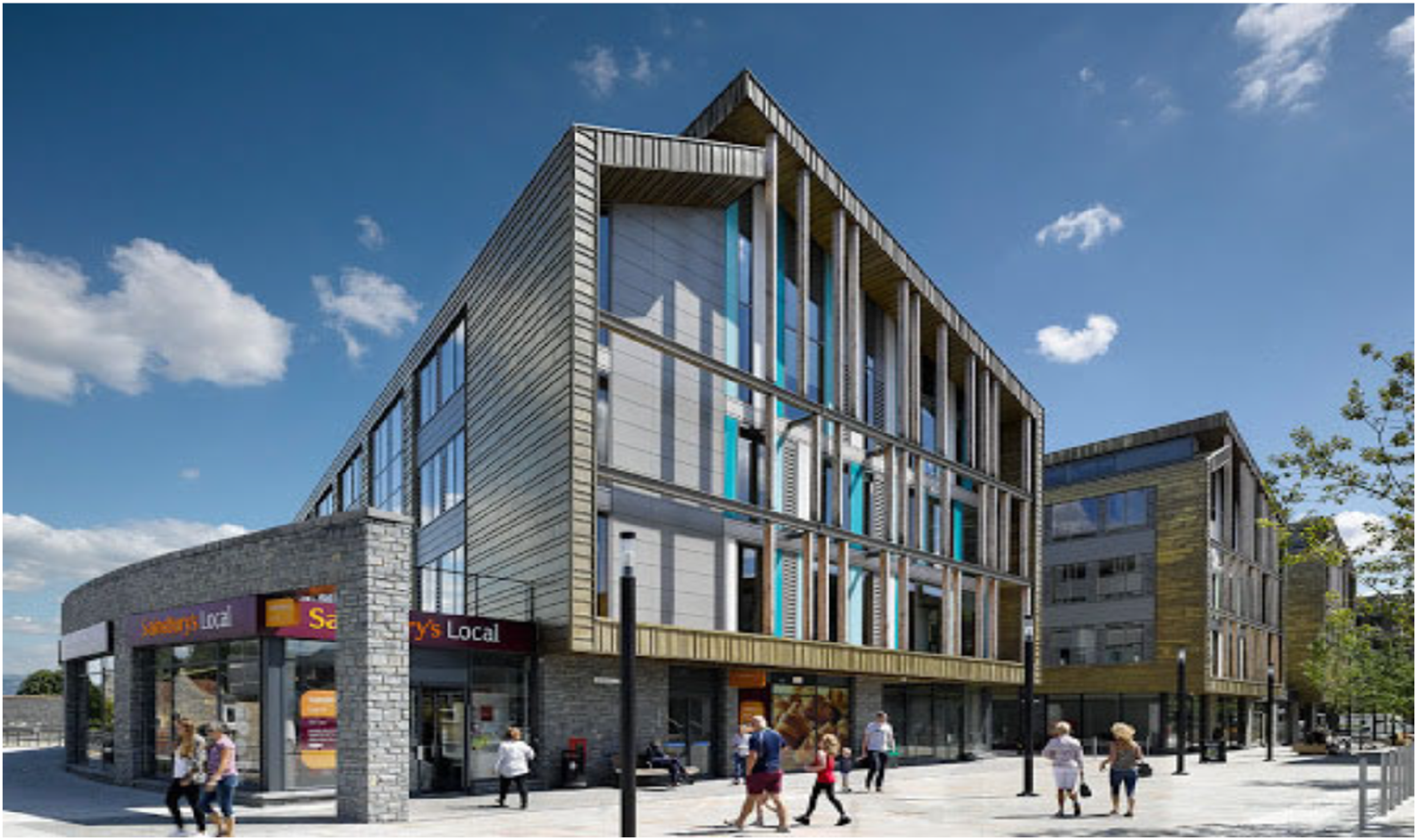

The office is a large building with variable operations and occupancy patterns which can be accurately modelled only by using a DSM modelling approach. The HVAC system in the office building, described in detail in later in the case study, is atypical and has complex controls. This means that a high level of detail in HVAC modelling and component-level energy breakdown is necessary. DSM with a detailed HVAC modelling approach was used in this case study. Detailed guidance on modelling approaches and tools is explained in TM54. ²

TM54 baseline

The baseline building generation is covered in TM54 from Steps 1 – 11. For each of the steps, model inputs must be defined along with ascertaining confidence levels in their assumptions to guide 5.0 Scenario/Sensitivity analysis.

Geometry and site details

Step 1: Constructing and building the model

Generating the model geometry and setting up site information is one of the first steps in undertaking building modelling and forms the basis from which all future calculations are undertaken. The process involves creating geometry, defining constructions, zoning, and selecting appropriate weather data. The accuracy and quality of these inputs in the model will in turn affect the accuracy of future model outputs.

For this case study, the building’s architectural design drawings are used to inform the inputs for geometry, construction, and zoning. Construction details are defined with material layers and typical year-hourly weather data from the nearest weather station is selected for the simulations. Figure 3 shows the model image. In the model, various space types, separated into zones are open office areas (69%), circulation (24%), toilets (4%), storerooms (1.5%), a server room (0.5%), and a plant room (0.5%).

Figure 3.

Model visualisation of the office building.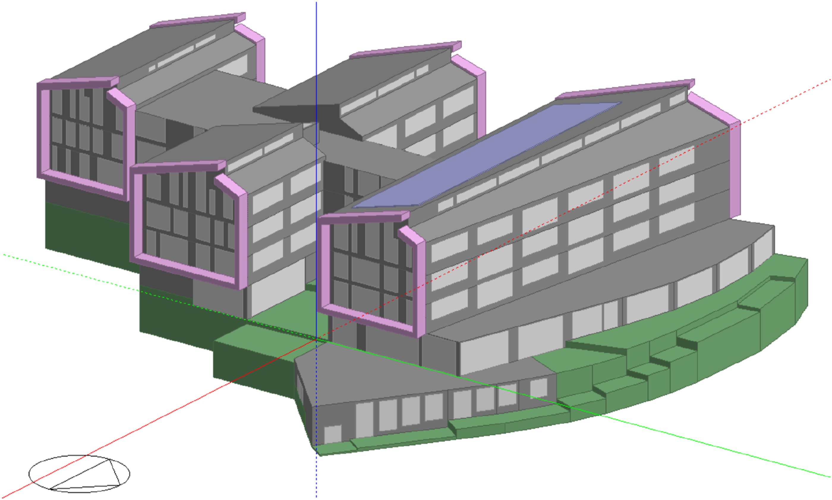

The building is designed for high energy efficiency and has low fabric U‐values. It has narrow floor plates, connected by atriums and cut-outs, creating an interconnected and open environment, has deep natural light penetration and enhances natural ventilation by creating a stack effect. Fabric properties are as follows: U‐values (W/m²K) for Wall: 0.20; Window: 1.4; Roof: 0.15; Ground: 0.15; and the design target for airtightness was 5 m³/hr/m² @ 50 Pa. Glazing has a g-value of 0.4 and a visible light transmission (VLT) of 0.69. ² Spaces are designed to have large windows for daylighting which are also partially operable for natural ventilation and free cooling in summer. The confidence level in the construction inputs is moderate, assuming that there are typically good practice construction methods being used. The variations in fabric-related simulation inputs will therefore be similar to typical buildings.

Operation details and internal gains

Building occupancy and other loads related to internal gains such as lighting and equipment along with the intended hours of operation of the plant and equipment must be established as far as possible. They are typically estimated by assessing the installed equipment and establishing the occupied and operating hours of the building and the way that the building is to be managed. While design documentation can provide the occupancy numbers and internal loads, information gathering from the intended occupiers (e.g. by conducting a structured interview) is the best way to establish the operation. In scenarios where this information is not readily available, typical building estimates can be used for the baseline modelling with a high degree of uncertainty for scenario and sensitivity analysis.

Data in the case study model about the occupancy and various internal gains are described per design stage documents and based on discussions with the client for loads and operation. Table 1 summarises the operation details and internal gains for the case study building. The rest of the section explains these model inputs in detail, covering each of the steps given in TM54.

Table 1.

Operation details and internal gains for the case study building.

Operation details	Description	Building detail	Remarks
Step 2: Occupancy	This covers gains due to people in the spaces defined by occupancy density and schedules. Indoor environmental quality and operating hours for other loads are often linked to occupancy. They are described in their respective sections	The building was designed for 455 persons, occupied during the weekdays only from 07:00 -19:00 with varying diversity per space type along with some out-of-hours usage Occupancy density also varies per space type such as 0.11 people/m2 for open office areas	Model inputs (density and schedules) for occupancy are set zone-by-zone. This enables the simulation of dynamically varying occupancy load effects and any ventilation control requirements
Step 3: Lighting	Lighting energy use and associated heat gains are estimated after defining its loads, operating hours, and controls	Lighting power density for key spaces is 5 W/m2. the building uses a background (mainly LED lamps) and a task lighting (CFL) scheme. Operations are as per occupancy with further controls using passive infra-red (PIR) and daylight sensors	Total energy use and associated heat gains for all these types of loads are estimated after defining their power ratings and operating hours As DSM modelling is granular, inputs for these loads are defined zone-by-zone with hourly varying time schedules This enables the estimation of their dynamically varying energy use and their effect on space-level heat balance
Step 4: Lifts and escalators	Lifts energy use can be calculated as a part of small power equipment or separately	Lift and other energy use associated with circulation areas are collectively modelled and their total load is assumed to be 1.30 W/m2
Step 5: Small power	This includes plug loads, which can be difficult to estimate, especially when the ultimate occupier is not yet known. Benchmark data can be helpful estimates at the design stage	Power density for equipment is 5.5 W/m2 and includes office equipment and an allowance for other miscellanies loads The operation schedule is as per the occupancy
Step 6: Catering	Kitchen, dining, and pantry areas can have their energy use calculated as separate end uses	A cafe on the first floor is part of a large common area with circulation. For simplification, the area is defined within circulation and therefore their energy use is spread across the circulation zones with an average load of 1.6 W/m2
Step 7: Server	Servers are high energy end use and can be metered separately	The server load of the building at peak occupied hours is 29 kW and the standby load is 15 kW
Step 8: Plant and equipment	Any additional loads and equipment that are not categorised above	Other building loads that could be attributed to these such as lifts, CCTV, and actuators, are added to small power
Step 9: Domestic hot water (DHW)	Evaluating the energy used to provide DHW requires estimating the amount of water used, schedules, system energy losses, and fuel sources. DHW does not affect the heat balance as such	This usage varies based on space type and at the design stage typical benchmarks are used, overall building average demand is set at 0.2 L/m2/day	DHW is provided in toilets by a heating system and by an electric point-of-use type system at the cafe and tea points

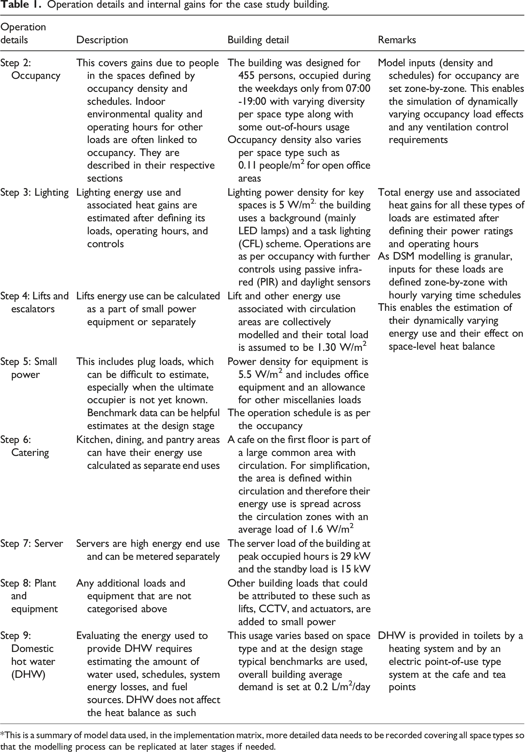
*This is a summary of model data used, in the implementation matrix, more detailed data needs to be recorded covering all space types so that the modelling process can be replicated at later stages if needed.

Step 2: Estimating operating hours and occupancy factors

The building is designed to have 455 people and will have dedicated desks in open office areas, the most common space type. The average occupancy density of these areas is 0.11 people/m². The circulation area’s occupancy density is assumed to be 0.05 people/m². The other space types are ancillary spaces and have occupancy densities ranging from 0.05 to 0.10 people/m². The typical weekday occupancy schedule for the building is presented in Figure 4 and the building is unoccupied during weekends. This is the typical occupancy, established after discussions with the building’s future occupiers in this owner-occupier office.

Figure 4.

Weekday occupancy schedules of the office building.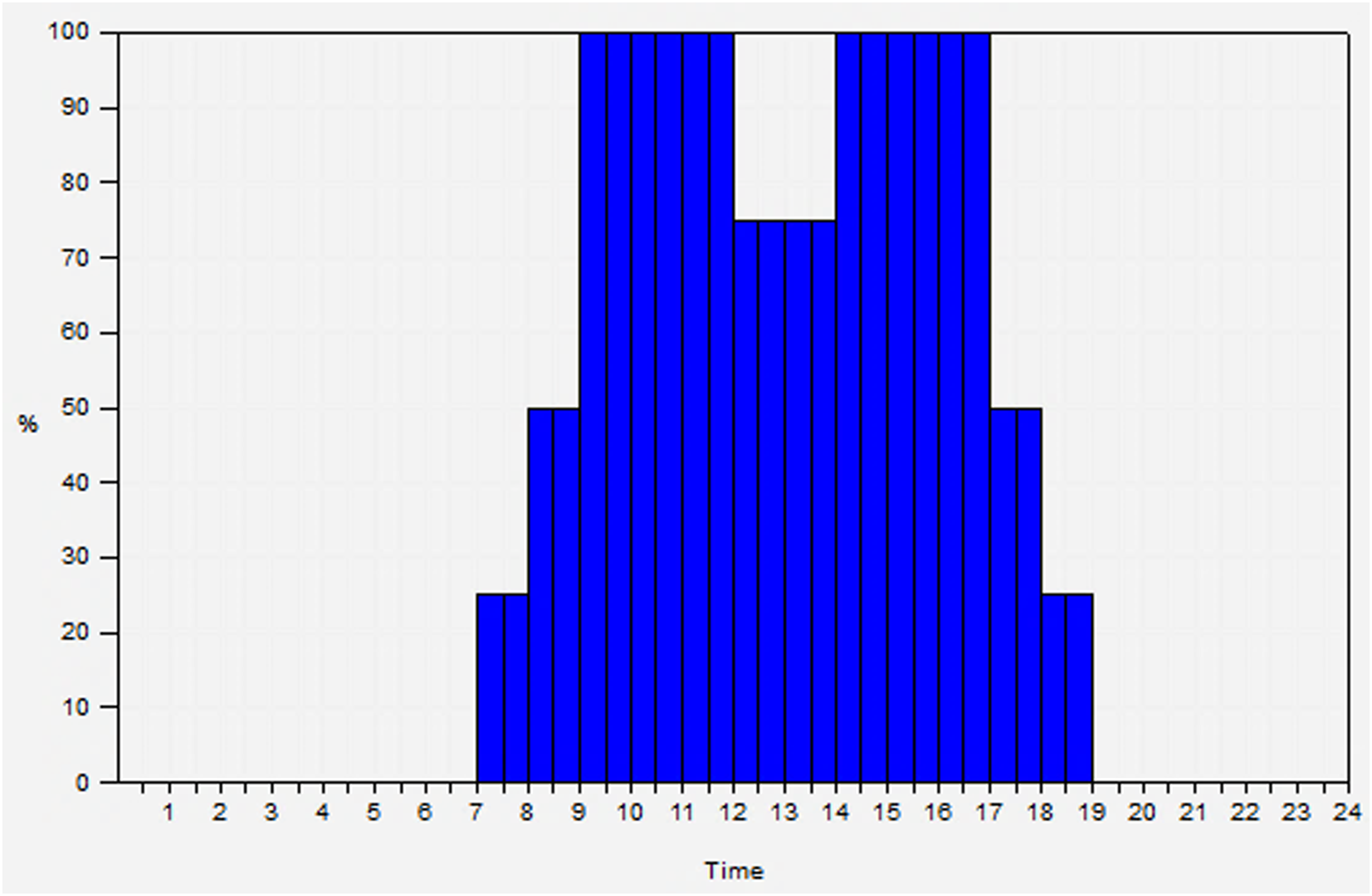

Step 3: Lighting

Lighting gains are based on planned lighting equipment. The building is planned to have a background (mainly LED) and a task lighting (CFL) scheme. Different target illuminance levels exist for places such as offices, stores, and toilets have 150 lux illuminance target and meeting rooms have a 400 lux target. Additionally, with manually operated lights, the target illuminance levels are 500 lux on desks. The weighted area average lighting power density is set to be 5 W/m². Its operation follows the occupancy schedule for each of the spaces.

Step 4: Lifts and escalators

There are multiple lifts in the building with a lift power consumption assumed as per design documents of 45Wh per journey. To simplify the calculations, Lift and other energy use associated with circulation areas are collectively modelled and their total load is assumed to be 1.30 W/m².

Step 5: Small power

The key end uses in the building, covered in small power include computers, printers, photocopiers, CCTV, and natural ventilation actuators. Small power use is assumed to follow the same schedule as occupancy with 5% standby loads. Total loads are defined as follows:

• 455 Workstations at 14W per thin client terminal and 33W for screen.

• Photocopiers. & Printers. In-Use: 207W. Standby: 12W

• CCTV + Access Control + Actuators etc: 2.2 kW, continuous.

The average power density for small power equipment is set to 5.5 W/m².

Step 6: Catering

The total catering base load is assumed as 3 kW. Catering facilities are part of common areas and therefore their energy use is spread across the circulation zones with an average load of 1.6 W/m².

Step 7: Server

The building server room’s planned capacity is set to be 29 kW which equates to 450 W/m². Its operation is set to be at full capacity during occupied hours with a standby load of 15 kW during non-occupied hours. Cooling loads for the server room are dependent on electrical loads and are accounted for in the heat-balance calculations in DSM software tools.

Step 8: Plant and equipment

The building does not have any significant additional equipment. The security system and any other plug loads are already added in step 5: small power section.

Step 9: Domestic hot water (DHW)

The typical consumption of hot water is calculated as 0.2 L/m²/day. The use of hot water is in the toilets using the heating system and electric point-of-use taps at tea points and cafe. The basis of estimation of the quantity of hot water use is:

• 5min shower/20 persons/day @4.5 L/min(HW) = 450 L/day showers.

• 1min hand wash/150person/day @1.4 L/min = 210 L/day.

• 1min hand wash/300person/day @2 L/min = 600 L/day.

Step 10: Adding internal heat gains to the model, for energy uses calculated outside the model

Table 1 covers all the model data inputs from operations and gains as per TM54 Steps two to Step 9. Following this, Step 10 requires adding internal heat gains to the model, for energy uses calculated outside the model. As the modelling process is undertaken by a DSM tool, the impact of internal gains on the heat balance is already included in the calculations. There were no additional energy uses that were calculated outside the model.

The confidence level in the occupancy-related factors (Steps 2-9) is low, similar to most buildings at the design stages. Therefore, a typical variation is expected to be seen in these inputs from what is estimated here and in the actual building. These variations can be up to ±10% as per BS EN 15,603:2008 ⁵ and have been used to inform the sensitivity analysis.

HVAC system definition

Figure 5 The energy use for HVAC systems and associated controls is required to be estimated and separately reported. This energy use should include all HVAC systems including heating and cooling, fans and pumps, and domestic hot water (unless calculated outside the model). Detailed HVAC modelling is where the system is modelled component by component.

Figure 5.

The HVAC system schematic for the case study building.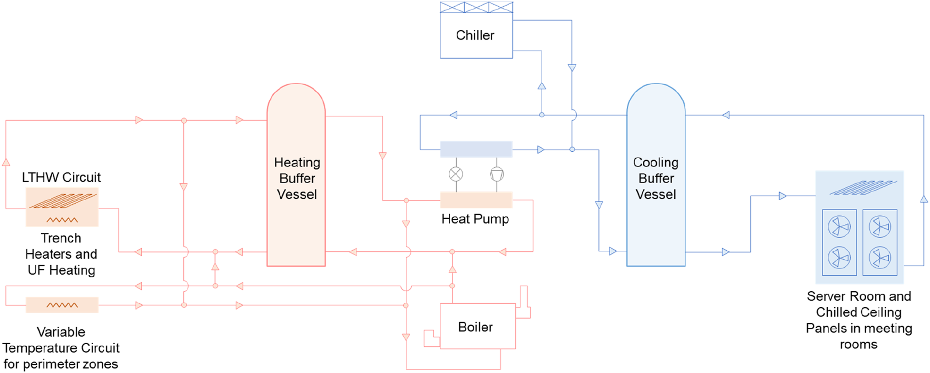

Figure 4 shows the schematic of the HVAC system planned for this building. The heat pumps are designed to satisfy the cooling needs of the IT server room and in turn, provide heating to the rest of the building. Heat pumps can produce simultaneous heating and cooling. The hot water and the chilled water are distributed via heating and cooling buffer vessels respectively. The heat pumps will only be operated if there is a heating demand in the building. When there is heating demand then, the server and meeting rooms’ cooling needs are met by the heat pump. The rejected heat from the cooling is used for building heating purposes. When the amount of heat produced by the heat pumps is insufficient for the building heat load, in the event of low external temperatures, then the additional heat needed will be provided by modular condensing gas‐fired boilers which were designed to meet peak loads and provide full back‐up. In the absence of heat demand, the heat pumps do not work and a free cooling chiller, where low external air temperature is used to assist in chilling water, satisfies the cooling needs. The heat pumps will have a maximum combined CoP (40% cooling/60% heating) of 6.5. The energy efficiency ratio (EER) (cooling mode, full load) will be 2.75 and the heating CoP (full load) will be 2.31. The boiler seasonal efficiency is assumed as 95.6%.

There are two heating loops planned, one constant temperature loop that runs at a fixed flow temperature of 45°C and a weather‐compensated variable temperature loop that runs at a maximum of 65°C during boost time. Underfloor radiant heating is provided in circulation and communal areas and trench heaters supply heating to all perimeter zones having offices and meeting rooms. Cooling for space conditioning, only provided for meeting rooms, is supplied by chilled beams.

Natural ventilation is the primary form of ventilation and is provided by vents which are controlled by a building management system (BMS), based on CO₂ concentration (opening threshold: 1500ppm) and air temperature (opening threshold: 24°C). A night‐cooling strategy is specified to keep the open‐plan offices cool in summer. Manually openable vents are also provided. Toilets and other enclosed occupied spaces have dedicated mechanical exhausts.

Building services operations are linked to occupancy patterns. The heating setpoint is set to be 19°C and in spaces where cooling is provided the cooling setpoint is set to 23°C.

Modelling for this system in this implementation route is carried out by using the Detailed HVAC modelling in DesignBuilder. Figure 6 shows the detailed HVAC schematic used in the simulation. The model incorporated a heat pump and a boiler as primary conditioning equipment with buffer vessels/storage tanks for storing hot and cold water. Free cooling modelled has been modelled via a cooling tower.

Figure 6.

Detailed HVAC system modelled in DesignBuilder.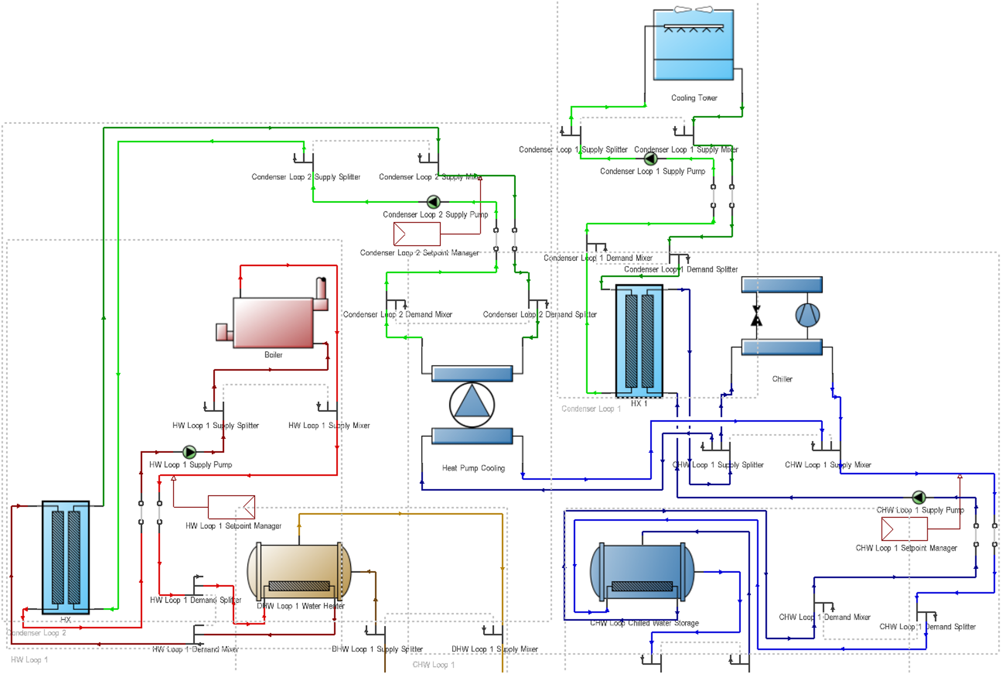

Few simplifications and minor adjustments had to be made in the simulated system components compared to the design, without affecting the overall strategy. Some of these are as follows:

• The original design layout was simplified to have only the key components which were ‘autosized’. This is a simpler and faster process of modelling and ensures that there is consistency in component sizing. The total auto-sized load of the system component was checked against the design estimates.

• Free cooling (air-cooled chiller with economisers) cannot be modelled as a standard component in EnergyPlus. Therefore, it was modelled as a waterside economiser using a cooling tower and heat exchanger.

• Heat exchangers have been used to connect some components which are not directly connectable in the software, such as to link two sources of heating at different temperatures.

• Hot water buffer vessel in EnergyPlus is designed for domestic water storage and therefore has a limitation of exit temperature to be a minimum of 55°C. As the lowest target temperature in the actual system is sometimes at 50°C this will result in slight auto-sizing errors, but overall energy use should remain less affected.

On-site renewables

On-site electrical generation (e.g., photovoltaics panels), if included in the model, can be helpful to identify a building’s net energy use and compare the generated energy against the building demand. This building has a rooftop PV installation of 210 kWp with an area of approximately 1000 m².

TM54 baseline results

As the key modelling inputs have been set up by Step 11, a simulation for the TM54 baseline performance projection can be run. The building’s energy use projection is calculated as 61 kWh/m²/annum with 15 kWh/m²/annum of site-generated solar PV energy use, resulting in net energy use of 46 kWh/m²/annum. Figure 7 shows the breakdown of this projected energy use, separated by end uses.

Figure 7.

TM54 Baseline energy use per end-use for the baseline building.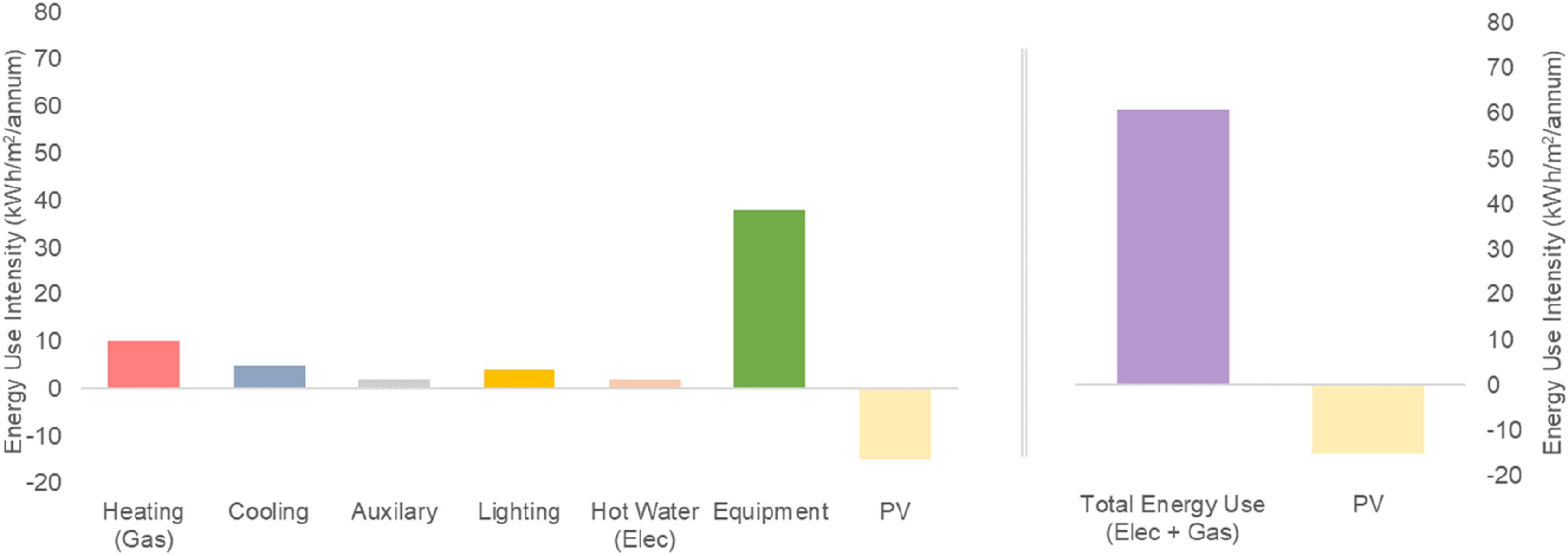

Heating, supplied by the rejected heat from the heat pump system as the primary heating, does not use any energy as that is the waste heat from the server room cooling process. Heating energy use shown in the graph above is the gas used by the backup boilers. The rest of the end-uses are fuelled by electricity. Space heating, equipment and server rooms account for a major proportion of energy use for the building. Cooling is provided for the servers and only in the meeting rooms, so its total energy use is low. Additionally, the use of natural ventilation for the provision of fresh air and natural cooling keeps the total energy use of the building rather low.

This is the central estimate of energy performance. However, for better communication of expected building performance, realistic scenarios that account for uncertainty in modelling assumptions should also be presented.

Scenario/sensitivity analysis

Performance projections at the design stage are prone to several operational risks. These risks can be due to management of the building after occupancy (Step 12) or functional changes that occur in the building over time. To account for these risks, when projecting energy use, a range of simulation runs should be undertaken. These runs should consider the variety of plausible potential real-world operating scenarios, focusing on those parameters which are least certain and/or are most influential. This allows quantification of the difference between ideal performance (Figure 7, at the end of Step 11) and how the building is likely to operate. This risk assessment can be done using a systematic approach of sensitivity and scenario analysis which can identify the most important and influential model inputs (Step 13) and quantify the total variability in the calculation results (Step 14).

As a part of the TM54 baseline modelling process (Steps 1-11), all key input parameters were tagged with the confidence level in their values. For this building, the impact of key model input parameters which are uncertain such as occupancy and internal gains or can significantly influence building performance such as construction quality and systems operations are explored in the sensitivity analysis. Table 2 lists all the uncertain variable categories, the model inputs that are changed, and their variation (lower limit, upper limit, and worst case) assumed in the sensitivity analysis. The variations are those that are assumed by modellers based on their experience, published literature,^5,6 and discussions with key stakeholders and building users. Parametric simulations run by changing multiple parameters are undertaken to ascertain the most important design inputs that cause variation in building performance from the central (TM54 baseline) estimate.

Table 2.

Design variables explored in the sensitivity analysis.

Variable category	Model input	Lower limit	Upper limit	Worst case	Remarks
Geometry	Wall U‐values	Val −10%	Val +10%	Val +20%	Potential issues with construction quality can lead to variations
	Window U-value	Val −10%	Val +10%	Val +20%
	Roof U-value	Val −10%	Val +10%	Val +20%
Occupancy	Occupancy density	Val −10%	Val +10%	Val +20%	This is a typical variation seen in occupant-related behaviour. Confidence is low in these variables because building usage evolves
Internal gains	Equipment power density	Val −10%	Val +10%	Val +20%
	Lighting power density	Val −10%	Val +10%	Val +20%
	Server capacity	Val −10%	Val +10%	Val +20%
DHW	DHW demand	Val −20%	Val +20%	Val +25%
HVAC	Heating setpoint	Val −1°C	Val +1°C	Val +2°C
	Cooling setpoint	Val +1°C	Val −1°C	Val −2°C
	Heating buffer vessel heat exchange efficiency	Val	Val −5%	Val −10%	Variation is possible due to commissioning and operation issues. The confidence level is moderate as the HVAC strategy is simple
	Cooling buffer vessel heat exchange efficiency	Val	Val −5%	Val −10%
Renewable energy system	PV panel efficiency	Val +10%	Val −10%	Val −20%	This variation is to factor in changes in the central estimate of PV panels installed due to any maintenance issues (e.g., not cleaning the panels over time)

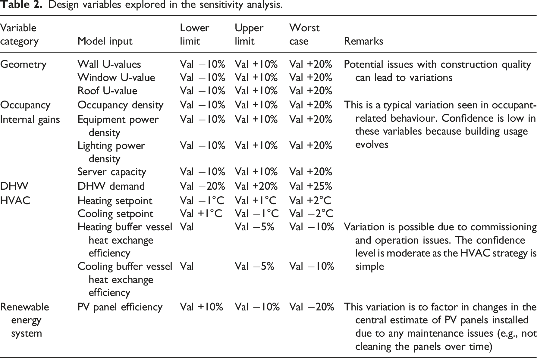
Regression-based parametric sensitivity analysis was undertaken by running 250 simulations and changing multiple variables at a time. This analysis assumes that design variables are independent of each other. Figure 8 shows the sensitivity analysis results for total building energy use, ranking the parameters from highest to lowest importance.

Figure 8.

Sensitivity analysis of variable input parameters on net energy use.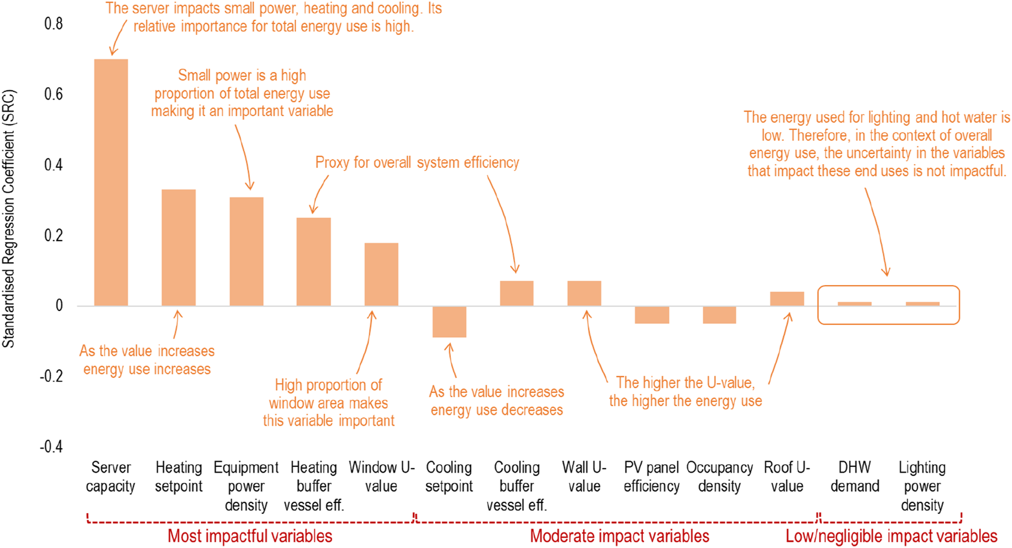

The variables with the highest standardised regression coefficient (SRC) are the most important. For example, within the range of variations assumed, the most influential parameters are server capacity, heating system efficiency and heating setpoints, equipment power density and window U-values. Server capacity is a significant factor here because not only does it affect the equipment energy use (the largest energy end-use), but also it has an impact on heating energy requirements, because if the server capacity decreases the free heat available decreases, resulting in an increase of heating energy from backup boilers. The direction of the SRC shows a direct or inverse relationship. For example, if the heating setpoint increases, the total energy use will increase, however, if PV panel efficiency increases the overall energy use decreases. To ensure that the building performs as intended or its performance improves further, these higher-ranking design variables are the inputs that will have the maximum impact.

Uncertainty is also calculated by varying all the input parameters in Table 2 within the ranges defined, the same set of simulations used in the sensitivity analysis above. Figure 9 shows the impact of variability (uncertainty) of all these inputs on individual end-uses and the net energy use. The total energy use of this case study building can range between 54 kWh/m²/annum and 72 kWh/m²/annum. Therefore, if the building is to perform as intended, the most influential parameters listed above would require close monitoring and safeguarding from significant changes.

Figure 9.

Uncertainty around TM54 baseline energy use for various end-uses.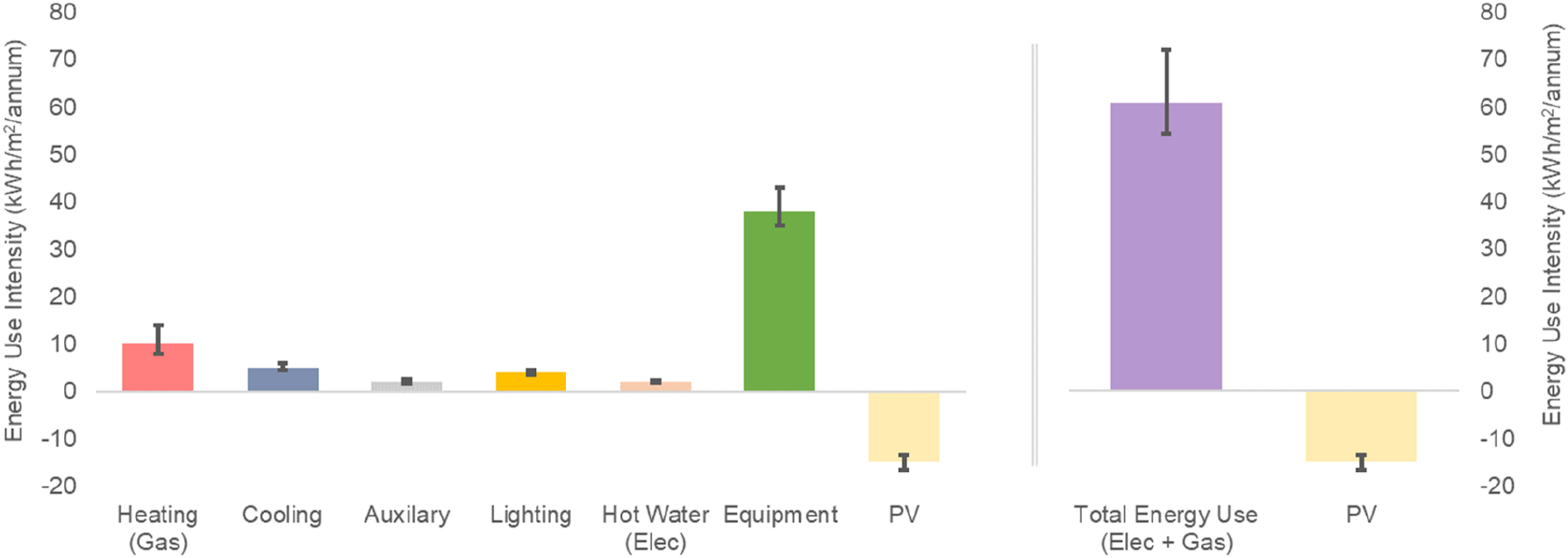

Besides the sensitivity and uncertainty analysis, two distinct scenario analyses were also undertaken:

(1) Future climate scenario,

(2) Worst-case scenario.

For future climate scenarios assessment, the ambient temperatures are expected to increase, leading to a reduction in the heating energy use of the building. Future climate scenario test is undertaken using 2050 weather data for high, medium, and low emission scenarios ³ and the total energy use projection is 57 kWh/m²/annum, 59 kWh/m²/annum and 60 kWh/m²/annum respectively. It should be noted that with increasing temperatures the building, not having comfort cooling for most of the spaces, may experience overheating in summer and this may necessitate the installation of a cooling system. Such an analysis can inform design decisions and recommendations for the long-term management of the school.

Besides the upper and lower range of likely building performance, the worst-case scenario energy use is also calculated as 94 kWh/m²/annum. This worst-case assumes a poorly managed building with the values under the worst-case column in Table 2 such as extended running hours, high occupancy, and high levels of internal loads. The current worst case is significantly higher than the central energy use projection and highlights the significance of managing the performance in use.

Reporting and benchmarking

Presenting simulation results in context and comparing them against benchmarks and building targets can be useful to determine whether the results are within an acceptable range. Figure 10 shows the comparison of TM54 baseline estimates against the good practice (25^th percentile) and typical (median) benchmarks as per the DEC database, ⁷ and CIBSE TM46 benchmarks. ⁸ It is seen that the TM54 central estimate is below good practice and typical benchmarks. This is the case also after factoring in the uncertainty (seen in Figure 9) and even the worst-case performance projection, meaning that the building design is resilient to change in the context of energy performance. However, to avoid underperformance, safeguards should be put in place to manage energy use during actual operation.

Figure 10.

Simulated energy use compared against industry benchmarks.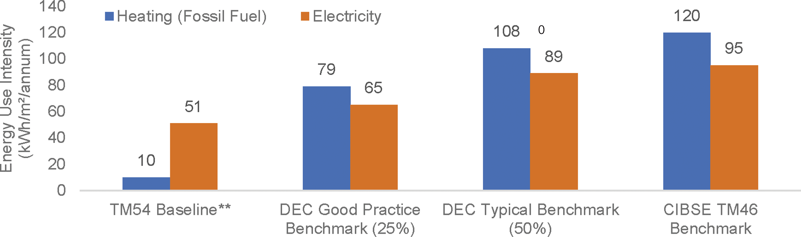

Result reporting for TM54 calculations should not just be limited to central estimates, as seen in Figure 7, but also include further results and assessments undertaken after uncertainty and sensitivity analysis along with a comparison against benchmarks. Reporting of modelling inputs and outputs in a structured implementation matrix (Annex A of CIBSE TM54 ² ) allows for documentation of all the assumptions that have been made alongside the results, at each modelling step. While this keeps the modelling process transparent, it also provides useful documentation for operational stage performance assessments.

Operational performance of the building

This case study is an example application for CIBSE TM54, which focuses on the design stage projection of energy use. These design calculations are based on the best estimates that are available to the modelling team during the design stage. The actual energy use can be very different, even when calculated with best practice modelling at the design stage. Using TM54 modelling steps the compliance gap ² can be eliminated but the performance gap can remain due to many changes that might happen in a building including those that cannot be estimated at the design stage. The underlying causes of an energy performance gap go beyond the scope of modelling in TM54 and its accuracy. These causes can be mapped to various factors across various construction stages. ⁹

The building’s energy use in the first year of operations is metered as 96 kWh/m²/annum. This is higher than the central estimate in ‘TM54 baseline results' section and also outside the uncertainty range calculated in ‘scenario/sensitvity analysis' section. The identification of the root causes of the deviation is beyond the scope of TM54 methodology and this case study document. These causes have been determined using CIBSE TM63 methodology ¹⁰ and described in a separate paper. ¹¹ CIBSE TM63: Operational performance: Modelling for evaluation of energy in use ¹⁰ provides a model calibration-based framework and a step-by-step guide for measurement and verification of energy performance in use. The framework is designed to determine the energy performance gap in operation concerning design calculations and identify the root causes of the gap. It builds upon the design stage modelling done as per TM54 and is the natural successor of this TM for modelling and diagnosing during post-occupancy evaluation. ¹²

Summary

The following are the key points emerging from the CIBSE TM54 energy projections for this case study building using dynamic simulation with detailed HVAC.

• Performance assessment of this office building, with variable operations and occupancy patterns can be more accurately modelled by using a DSM tool.

• The HVAC system in the office building, is atypical and has complex controls. This means that DSM with a detailed HVAC modelling approach with component-level energy breakdown is necessary.

• Step-by-step modelling as per TM54, factoring in all energy end uses and operational details resulted in an energy use projection of 61 kWh/m²/annum.

• Sensitivity tests show that the building performance is highly susceptible to underperformance and variations in server room loads and system operation. A key risk that needs to be considered and managed is the risk of summertime overheating in the future as the ambient temperatures rise.

• Within reasonable uncertainty of model inputs and operational changes, the total energy use of this case study building can range between 54 kWh/m²/annum and 72 kWh/m²/annum. However, in case of severe mismanagement and operational issues, this can increase to 94 kWh/m²/annum.