Sage Journals: Discover world-class research

Abstract

We investigate the causal effects of religious service attendance on prosocial behaviours using longitudinal data from a nationally representative sample of 33,198 New Zealanders collected between 2018 and 2021. Our study innovates in three ways: (1) we use longitudinal rather than cross-sectional data; (2) we incorporate measures of help received alongside self-reported giving; and (3) our statistical models are designed to address causal questions, rather than simply to describe change over time. We model causal contrasts for three hypothetical interventions – increasing, decreasing, or maintaining religious service attendance – and assess their effects on eight distinct prosocial domains. Study 1 focuses on self-reported charitable donations and volunteering. Studies 2 and 3 examine receiving help – both personal and financial – from family, friends, and the wider community. Across all analyses, we find that the causal effects of religious service attendance are notably smaller than cross-sectional correlations suggest. However, even modest increases in regular attendance would result in charitable donations equivalent to approximately 4% of the New Zealand Government’s annual spending – a considerable public benefit. By applying robust methods for causal inference to national-scale panel data, our study provides insights that can inform public policy about the social functions of religious participation and advances a methodological framework for investigating the social consequences of cultural practices.

Keywords

causal inference charity church cooperation cross-validation DAGs longitudinal machine learning religion semi-parametric targeted learning TMLE volunteering

Introduction

A central question in the scientific study of religion is whether religion fosters prosociality (De Coulanges, 1903; D. D. Johnson, 2005; Norenzayan et al., 2016; Schloss & Murray, 2011; Sosis & Bressler, 2003; Swanson, 1967; Watts et al., 2015, 2016; Wheatley, 1971; Whitehouse et al., 2023). However, quantifying causal effects for religion presents significant challenges (Major-Smith, 2023). Investigators have limited scope to randomise supernatural beliefs, community worship, and personal prayer. On the other hand, valid causal inferences from non-experimental, ‘real-world’ data require the integration of high-resolution, repeated-measures time-series data with appropriate causal inference methodologies. Few studies succeed in this integration. A recent survey of the religion and prosociality literature reveals that nearly all non-experimental studies examining the links between prosociality and religion, including several longitudinal studies, remain correlational (Kelly et al., 2024). Currently, studies using longitudinal (panel) data have not leveraged their repeated measures to derive reliable causal inferences.

Here, to obtain causal inferences from time-series data, we utilise comprehensive panel data from 33,198 participants in the New Zealand Attitudes and Values Study (NZAVS) spanning 2018 to 2021. We quantify the effects of clearly defined interventions in religious attendance across the population of New Zealand, assessing eight outcome domains related to charitable financial donations and volunteering. We obtain causal inferences by contrasting expected population averages under different modified treatment policies (Díaz et al., 2023; Haneuse & Rotnitzky, 2013; Hoffman et al., 2023).

Our initial causal contrast investigates: ‘What would be the average difference in each of the eight prosocial outcomes across the New Zealand population if everyone attended religious services regularly (at least four times per month) compared to if no one attended?’ This theoretical inquiry simulates a hypothetical experiment with random assignment to either regular attendance or complete non-attendance, mirroring the all-or-none contrast that is commonly used in experimental designs (Hernán et al., 2016).

A second causal contrast investigates: ‘What would be the average difference in each of the eight prosocial outcomes across the New Zealand population if everyone attended religious services regularly (at least four times per month) compared to maintaining current attendance levels?’ In this analysis, we compare the expected prosocial outcomes under regular religious service attendance (at least four times per month) with outcomes observed under existing attendance patterns. This causal contrast may inform practical policies aimed at influencing non-regular attendees who might stop attending religious services.

Our third causal contrast examines: ‘What would be the average difference in each of the eight prosocial outcomes across the New Zealand population if no one attended religious services compared to maintaining current attendance levels?’ In this analysis, we compare the expected prosocial outcomes in a scenario where all religious service attendance ceases with the outcomes observed under existing attendance patterns. This causal contrast may inform practical policies aimed at influencing regular attendees who might discontinue their participation in religious services.

Although the set of causal contrasts investigators might consider is theoretically limitless, the contrasts that we have selected address our targeted scientific and policy interests.

Importantly, our approach does not centre on testing specific hypotheses; rather it is designed to accurately and consistently compute our stated causal contrasts (Hernán & Greenland, 2024).

Method

Sample

Data for this study were collected as part of the New Zealand Attitudes and Values Study (NZAVS), an annual longitudinal national probability panel that assesses New Zealand residents’ social attitudes, personality, ideology, and health outcomes. The study has obtained responses from 72,910 participants since it started in 2009. The study operates independently of political or corporate funding and is based at a university. Data summaries for all measures used in this study are provided in Supplemental Appendices B–D: https://osf.io/vxd6m/. For more information about the NZAVS, visit: OSF.IO/75SNB.

The data analysed in this study were obtained from the NZAVS waves 10–12 cohort, covering the years 2018–2021. This is the largest cohort in the NZAVS. Although this cohort was obtained through national probability sampling and closely approximates the New Zealand population, we applied weights based on the 2018 New Zealand Census estimates for age, gender, and ethnicity to further enhance representativeness. Detailed information on these survey weights is available in the NZAVS documentation at OSF.IO/75SNB.

Treatment indicator

We assessed religious service attendance using the following question:

Do you identify with a religion and/or spiritual group? If yes, how many times did you attend a church or place of worship during the last month?

Responses were rounded to the nearest whole number. Because few participants reported attending more than eight times, we capped responses above eight at eight (refer to Online Supplement Appendix B: https://osf.io/vxd6m/).

Measures of prosociality

We assessed prosocial behaviour using the following measures:

Study 1: self-reported charity

Participants reported:

Volunteering: Please estimate how many hours you spent doing each of the following things last week . . . Volunteer/charitable work.

Annual Charitable Financial Donations: How much money have you donated to charity in the last year?

Study 2: help received from others in the last week: time

Participants estimated the amount of help they received in the past week in hours from:

Family . . . TIME (hours)

Friends . . . TIME (hours)

Community . . . TIME (hours)

Owing to high variability, we transformed responses into binary indicators: 0 = none; 1 = any.

Study 3: help received from others in the last week: money

Similarly, participants were asked:

Participants estimated the monetary help they received in the past week from:

Family . . . MONEY (dollars)

Friends . . . MONEY (dollars)

Community . . . MONEY (dollars)

Again, owing to high variability, responses were converted to binary indicators: 0 = none; 1 = any.

Studies 2 and 3 employ revealed measures of prosocial exposure to minimise self-presentation bias. We assume that if religious institutions foster prosociality, initiating regular attendance would increase exposure to prosocial behaviours. This approach allows us to infer prosociality using help-recieved responses as a measure. The help-received measure is less susceptible to self-presentation biases that might otherwise distort the association between religious attendance and genuine prosociality. Furthermore, including baseline outcomes and treatments in our analyses mitigates the threat of undirected correlated errors.

Comprehensive details of all measures are provided in Online Supplemental Materials: Appendix A: https://osf.io/vxd6m/.

Causal interventions

We defined three targeted causal contrasts based on pre-specified modified treatment policies:

Regular Religious Service Treatment: assumes that everyone attends religious services regularly, defined as at least four times per month. In this scenario, individuals who currently attend less than four times per month have their attendance increased to four times, while those already attending four or more times per month remain unchanged.

Zero Religious Service Treatment: assumes that no one attends religious services. Here, individuals who currently attend more than zero times per month have their attendance reduced to zero, whereas non-attendees remain unchanged.

The Status Quo: no treatment is applied. We retain each individual’s observed level of religious service attendance without modification.

Causal contrasts

Based on these policies, we computed three causal contrasts:

Regular vs Zero Religious Service Attendance: this contrast compares average prosocial outcomes in a society where everyone attends religious services regularly to one where no one attends. It simulates a hypothetical experiment where individuals are randomised to either regular attendance or no attendance, allowing us to assess differences in prosociality one year after the intervention.

Regular Religious Service Attendance vs The Status Quo: this contrast compares average prosocial outcomes in a society where everyone attends religious services regularly to the current state. It contrasts the causal effect of transitioning non-regular attendees to regular attendance.

Zero Religious Service Attendance vs The Status Quo: this contrast compares average prosocial outcomes where no one attends religious services to the current state. It examines the causal effect of entirely eliminating religious service attendance from society.

Identification assumptions

To consistently estimate a causal effect, investigators must satisfy three assumptions (refer to Bulbulia, 2024b):

Causal consistency: potential outcomes correspond to the observed outcomes under the treatments in our data. We assume that conditional on measured covariates, potential outcomes do not depend on how the treatment was administered (VanderWeele, 2009; VanderWeele & Hernan, 2013).

Conditional exchangeability: conditional on observed covariates, treatment assignment is independent of the potential outcomes being compared (i.e. there is no unmeasured confounding) (Chatton et al., 2020; Hernan & Robins, 2024).

Positivity: every individual has a non-zero probability of receiving each treatment level, regardless of their covariate values. We evaluated this by examining changes in religious service attendance from baseline to the treatment wave (Westreich & Cole, 2010).

Target population

Our target population comprises New Zealand residents represented in the baseline wave of the NZAVS during 2018–2019, weighted by 2018 New Zealand Census data for age, gender, and ethnicity (Sibley, 2021). Although the NZAVS is a national probability study designed to reflect the broader New Zealand population, it tends to under-sample males and individuals of Asian descent and over-sample females and Māori (the indigenous people of New Zealand). To address these disparities and enhance the accuracy of our findings, we applied survey weights adjusting for age, gender, and ethnicity. Survey weights were integrated into our statistical models using the weights option in the ‘lmtp’ package (Williams & Díaz, 2021), following protocols described by Bulbulia (2024e). Note that the sample in this study is a single cohort, enrolled in the NZAVS in NZAVS wave 10 and NZAVS wave 11, and which may have been lost to follow-up in NZAVS wave 12.

Eligibility criteria

Participants were included in the analysis if they:

Were enrolled in the 2018 wave of the NZAVS (Time 10).

Provided responses to the religious service attendance question at both Time 10 (baseline) and Time 11 (treatment wave).

Participants with missing covariate data at baseline were included, with missing data imputed using information available at baseline. Participants may have been lost to follow-up by the end of the study (Time 12); we adjusted for attrition and non-response using censoring weights, as described below.

A total of 33,198 individuals met these criteria and were included in the study.

Missing data

We adopted the following strategies for handling missing data:

Baseline missingness

We used the predictive mean matching algorithm from the mice package in R (Van Buuren, 2018) to impute missing baseline data (<2% of covariate values). We performed single imputation, using only baseline data for imputation (Zhang et al., 2023).

Outcome missingness

To account for confounding and selection bias from missing responses and panel attrition, we applied censoring weights obtained using nonparametric machine-learning ensembles via the ‘lmtp’ package in R (Williams & Díaz, 2021).

Confounding control

To address confounding, we employ a modified disjunctive cause criterion (VanderWeele, 2019), which involves:

Identifying all common causes of both the treatment and outcomes.

Excluding instrumental variables that affect the exposure but not the outcome.

Including proxies for unmeasured confounders affecting both exposure and outcome.

Controlling for baseline exposure and baseline outcome, serving as proxies for unmeasured common causes (VanderWeele et al., 2020).

The covariates included for confounding control are detailed in Supplement: Appendix B. These methods adhere to the guidelines provided by Bulbulia (2024e) and were pre-specified in our study protocol https://osf.io/ce4t9/.

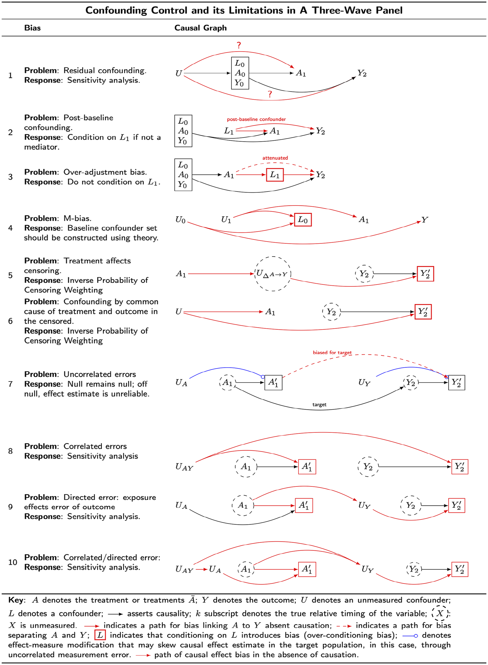
Figure 1 presents a causal diagram of our identification strategy. The graphs are labelled $G_{x}$ , where $x$ corresponds to a numbered row in the figure.

Figure 1.

Ten causal-directed acyclic graphs clarify distinct threats to valid causal inference in a three-wave panel study.

Figure 1 $G_{1}$ shows that by including measures of the baseline treatment and baseline exposure, along with all common causes, any unmeasured confounding would need to be orthogonal (i.e., statistically independent) to these baseline measurements (refer to VanderWeele et al., 2020). However, because treatments have not been randomised, the threat of orthogonal confounding persists. Specific threats are presented in $G_{1} - G_{10}$ . As described below, we address these threats by reporting sensitivity analyses that clarify how much unmeasured confounding would be necessary to explain away a result.

Figure 1 $G_{2}$ shows that if a confounder is measured in the treatment wave ( $L_{1}$ ), and it is known that this confounder cannot be affected by the treatment, we should adjust for it in our model.

In contrast, Figure 1 $G_{3}$ presents the threat of mediator bias. Since the treatment and confounders are measured simultaneously in each wave, including confounders measured in the treatment wave may bias results. To avoid such biases, we restricted confounders in our model to those measured in the baseline wave. We performed sensitivity analyses to address the worry of orthogonal confounding presented in Figure 1 $G_{2}$ .

Figure 1 $G_{4}$ presents examples of over-conditioning bias, which occurs when a baseline variable that is not a confounder is included but becomes a confounder when conditioned upon. To avoid such biases, we used theory to construct our set of confounders, following VanderWeele’s modified disjunctive cause criterion (VanderWeele, 2019).

Figure 1 $G_{5}$ and $G_{6}$ shows threats to valid inference arising from attrition. For example, if changes in religious status were to affect whether a participant remains in the study, or if there were a common cause of treatment and outcome in the censored data, our causal effect estimates could be biased.

Figure 1 $G_{7}$ – $G_{10}$ shows threats to valid causal inference from measurement error. If the errors in the treatment and outcome are uncorrelated ( $G_{7}$ ), the results will not generally be biased (though see Bulbulia, 2024d). However, if there were a common cause of bias in reporting both religious service attendance and charitable giving/volunteering (correlated errors, $G_{8}$ ), or if increasing/decreasing religious service were to affect the errors in reported charitable giving or volunteering (directed error, $G_{9}$ ), or both ( $G_{10}$ ), causal effect estimates could be biased. Again, sensitivity analysis helps clarify the robustness of our results to such biases. For primers on causal graphs, see (Bulbulia, 2024b, 2024d; Hernan & Robins, 2024; Suzuki et al., 2020). We reconsider the implications of measurement error biases in the discussion.

Statistical estimation

We used targeted minimum loss-based estimation (TMLE) to estimate causal effects from the observed panel responses (Van der Laan, 2014; Van der Laan & Gruber, 2012). Specifically, we used an implementation of TMLE that employs machine-learning algorithms to produce efficient statistical estimates for features of the data relevant to estimating our causal estimands from data. These algorithms do not make assumptions about the distributions of the data and are able to learn efficiently even in the presence of high-dimensional data such as ours.

We conducted our estimations using the ‘lmtp’ package in R (Williams & Díaz, 2021), utilising the SuperLearner library with predefined algorithms: ‘SL.ranger’, ‘SL.glmnet’, and ‘SL.xgboost’ (Chen et al., 2023; Polley et al., 2023; Wright & Ziegler, 2017). To ensure robust model performance, we employed 10-fold cross-validation, which guarantees that the data used for training the models are distinct from those used for testing. We produced graphs, tables, and output reports using the ‘margot’ package (Bulbulia, 2024a).

Sensitivity analysis using the E-value

To assess the robustness of our results to unmeasured confounding, we report VanderWeele and Ding’s ‘E-value’ in all analyses (VanderWeele & Ding, 2017). The E-value quantifies the minimum strength of association, on the risk ratio scale, that an unmeasured confounder would need to have with both the exposure and the outcome – after considering all measured covariates – to explain away the observed exposure–outcome association (Linden et al., 2020; VanderWeele et al., 2020). We used the bound of the E-value 95% confidence interval closest to 1 to evaluate the strength of evidence. We note that the E-value presents an approximation of confounding risk.

Scope of interventions

To illustrate the magnitude of the interventions, we present histograms (Figure 2) showing the distribution of religious service attendance during the treatment wave. In Figure 2(a), the intervention for regular religious service affects a more significant portion of the sample than the zero religious service intervention depicted in Figure 2(b). The ‘Regular vs Zero’ comparison addresses the question: what is the difference in effects between a society where religious service is universal compared to one in which religious service is completely absent?

Figure 2.

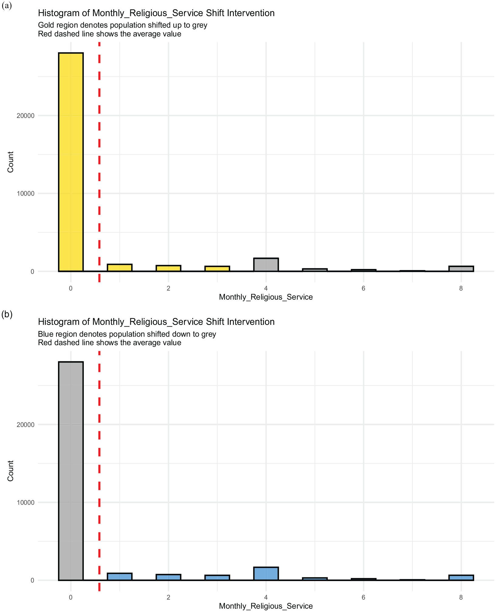
This figure shows a histogram of responses to religious service frequency in the baseline + 1 (i.e. the treatment) wave. Responses above eight were assigned to eight, and values were rounded to the nearest whole number. The red dashed line shows the population average. (a) Responses in the gold bars are shifted to four on the regular religious service intervention. All those responses in grey (four and above) remain unchanged. (b) On the zero-intervention, responses in the blue bars denote those shifted under the zero-intervention treatment.

Changes in religious service attendance

Table 1 shows the transitions in religious service attendance from baseline to the treatment wave. Assessing changes in the treatment variable is essential for evaluating the positivity assumption of causal inference, which, as stated above, requires that every individual has a non-zero probability of receiving each treatment level, regardless of their covariate values (Danaei et al., 2012; Hernan & Robins, 2024; VanderWeele et al., 2020). Although causal inference does not rely on the assumption that every combination of covariate and exposure is realised, where such observations are absent, stronger modelling assumptions are required. We observe that attendance levels at 0 (no attendance) and 4 (weekly attendance) were the most common responses and, furthermore, that there was indeed a change in attendance over time. That is, at the population level, we find changes in reported attendance between the baseline wave and the exposure wave occurred in the data.

Table 1.

This transition matrix captures stability and change in religious service between the baseline and treatment wave.

From	State 0	State 1	State 2	State 3	State 4	State 5	State 6	State 7	State 8
State 0	26,762	405	174	71	126	26	13	8	68
State 1	647	235	85	44	46	5	2	3	10
State 2	236	105	188	104	96	12	13	2	21
State 3	112	54	110	164	173	18	8	4	15
State 4	150	71	127	205	881	124	64	16	91
State 5	24	7	17	17	145	61	25	7	33
State 6	14	5	13	17	84	22	29	5	37
State 7	9	0	6	3	16	6	9	6	19
State 8	74	14	17	14	105	34	42	17	351

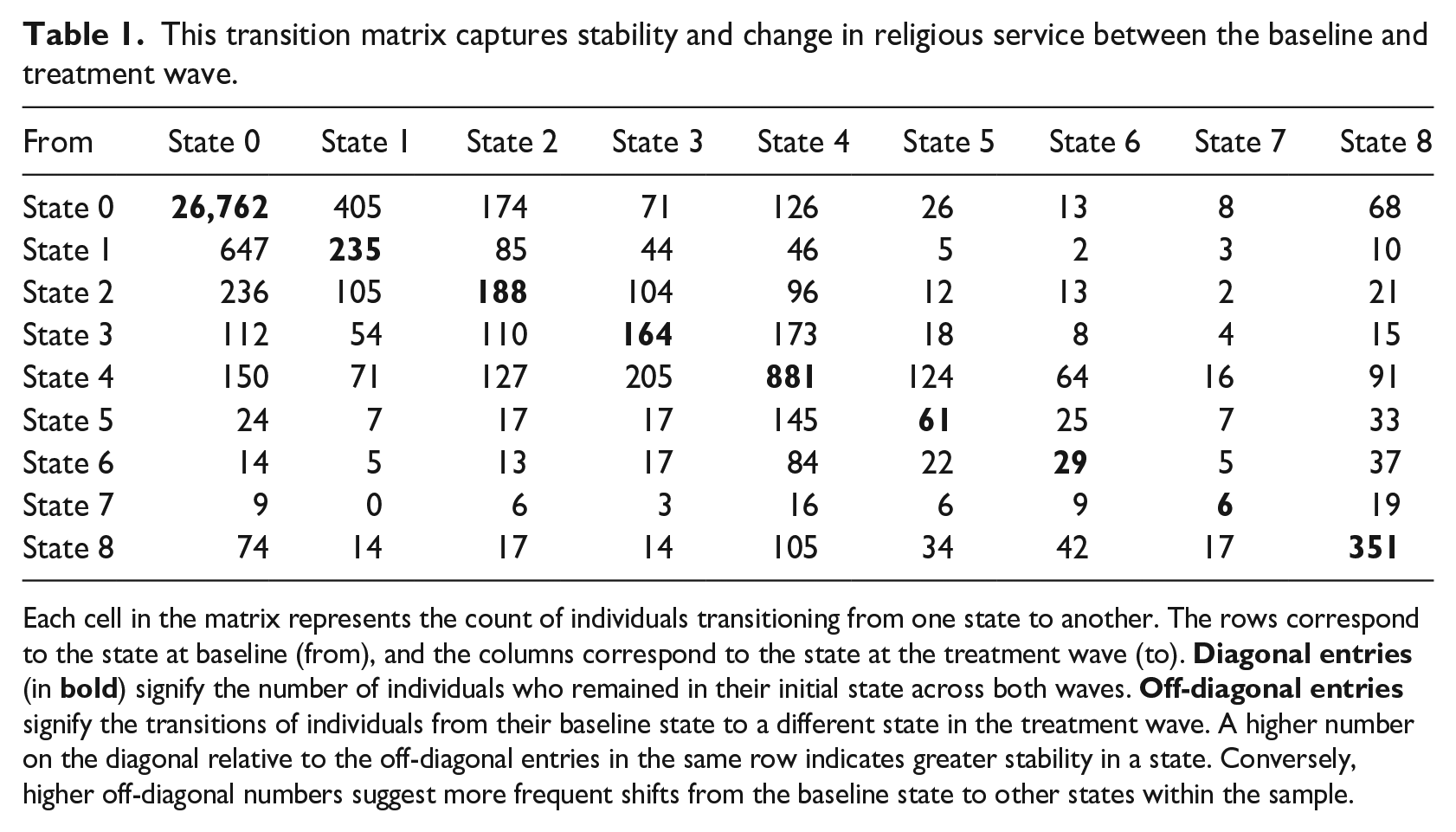
Each cell in the matrix represents the count of individuals transitioning from one state to another. The rows correspond to the state at baseline (from), and the columns correspond to the state at the treatment wave (to). Diagonal entries (in bold) signify the number of individuals who remained in their initial state across both waves. Off-diagonal entries signify the transitions of individuals from their baseline state to a different state in the treatment wave. A higher number on the diagonal relative to the off-diagonal entries in the same row indicates greater stability in a state. Conversely, higher off-diagonal numbers suggest more frequent shifts from the baseline state to other states within the sample.

Results

Study 1: causal effects of regular church attendance on self-reported volunteering and self-reported volunteering and donations

Regular religious service versus zero treatment contrast for donations and volunteering

Results for the treatment contrasts between Regular Religious Service and Zero Religious Service, focusing on self-reported volunteering and charitable donations, are displayed in Figure 3(a) and Table 2. These results are estimated on the causal difference scale.

Figure 3.

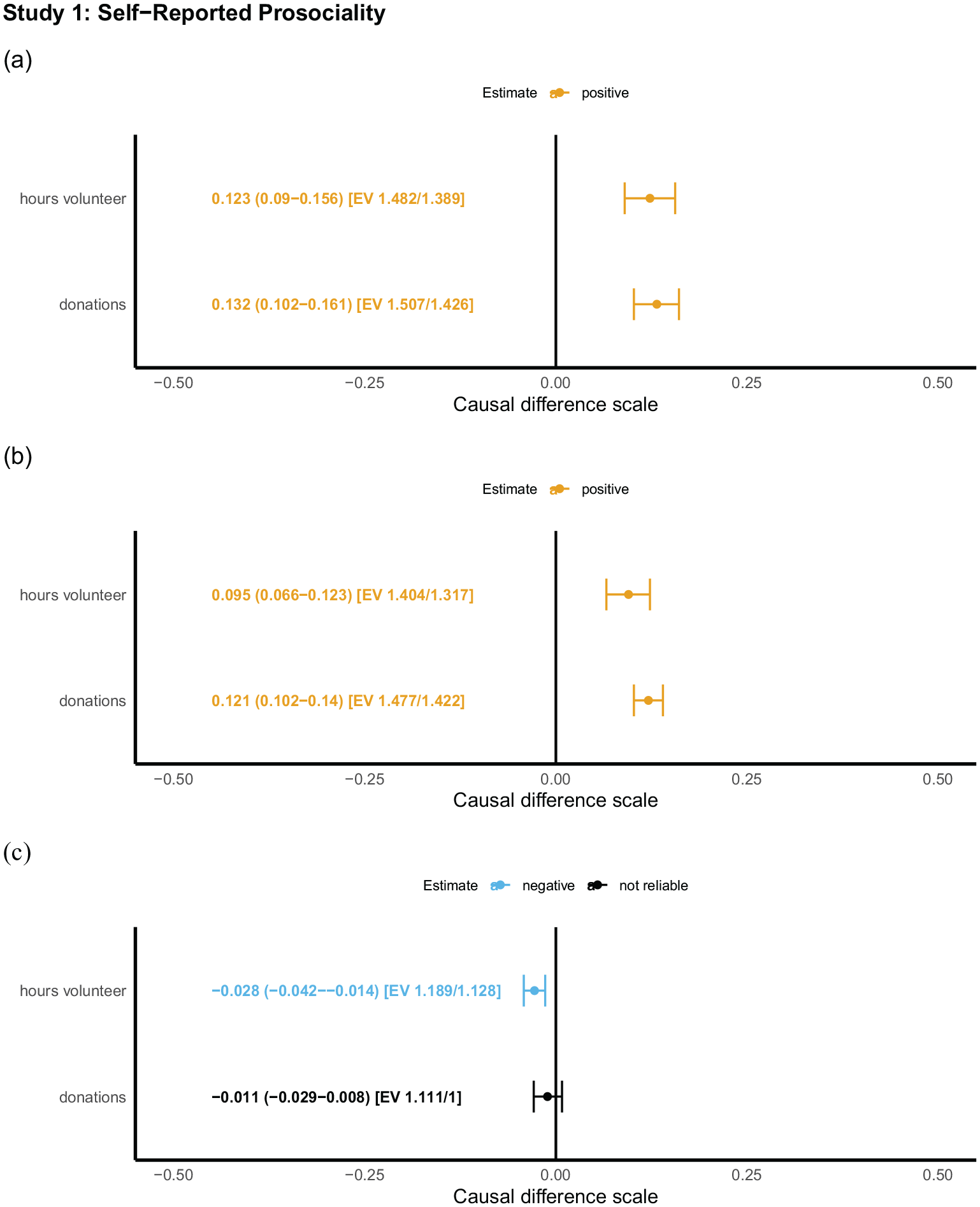
This figure graphs the results of model estimates for the three causal contrasts of interest on reported charitable behaviours at the study’s end. The causal contrasts are: (a) Regular versus Zero Religious Service, (b) Regular Religious Service versus Status Quo, and (c) Zero Religious Service versus Status Quo. Contrasts are expressed in standard deviation units.

Table 2.

This table reports the results of model estimates for the causal effects of a universal gain of weekly religious service vs a universal loss of weekly religious service on reported charitable behaviours at the end of the study. Contrasts are expressed in standard deviation units.

	E(Y(1)] − E[Y(0)]	2.5%	97.5%	E-Value	E-Value bound
Donations	0.132	0.102	0.161	1.507	1.426
Hours volunteer	0.123	0.090	0.156	1.482	1.389

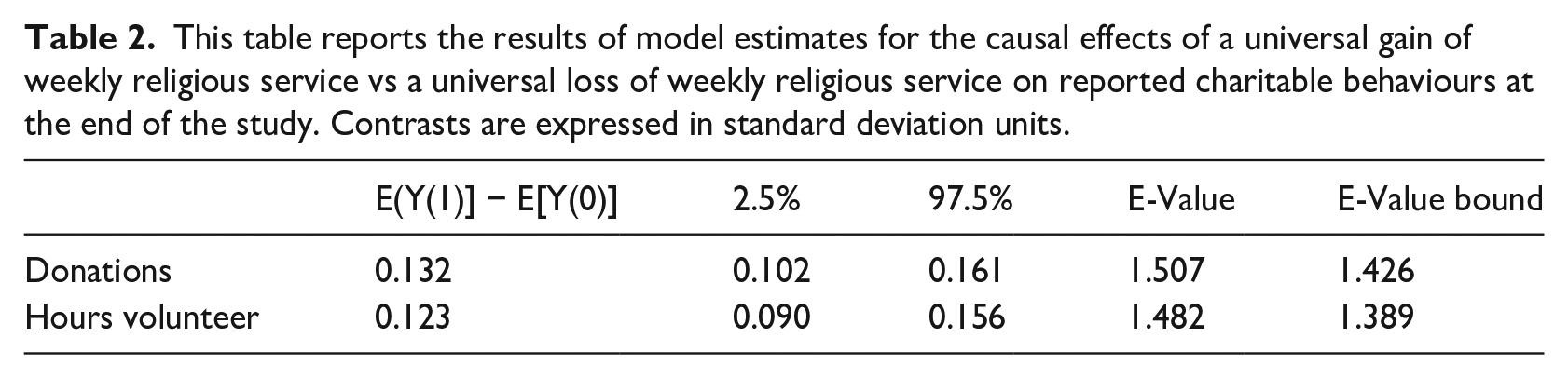
For donations, the effect estimate is 0.132 [0.102, 0.161]. The E-value for this estimate is 1.507, with a lower bound of 1.426. At this lower bound, unmeasured confounders would need a minimum association strength with both the intervention sequence and outcome of 1.426 to negate the observed effect. Weaker associations would not overturn it. We infer evidence for causality. On the data scale, this intervention represents a difference of NZD 656.58 per adult per year in charitable giving compared with the zero attendance intervention.

The effect estimate for hours volunteered is 0.123 [0.09, 0.156]. The E-value for this estimate is 1.482, with a lower bound of 1.389. We infer evidence for causality. On the data scale, this intervention represents a difference of NZD 30.21 minutes per adult per week in volunteering compared with the zero attendance intervention.

Regular religious service versus status quo treatment contrast for donations and volunteering

Figure 3(b) and Table 3 present results for the treatment contrasts between regular religious service and status quo, focusing on self-reported volunteering and charitable donations. These results are estimated on the difference scale.

Table 3.

This table reports results of model estimates for the causal effects of a universal gain of weekly religious service attendance vs the status quo on reported charitable behaviours at the end of the study. Contrasts are expressed in standard deviation units.

	E(Y(1)] − E[Y(0)]	2.5%	97.5%	E-Value	E-Value bound
Donations	0.121	0.102	0.140	1.477	1.422
Hours volunteer	0.095	0.066	0.123	1.404	1.317

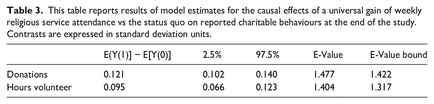
For donations, the effect estimate is 0.121 [0.102, 0.14]. The E-value for this estimate is 1.477, with a lower bound of 1.422. At this lower bound, unmeasured confounders would need a minimum association strength with both the intervention sequence and outcome of 1.422 to negate the observed effect. Weaker confounding would not overturn it. We infer evidence for causality. On the data scale, this intervention represents an increase of NZD 601.87 per adult per year in expected charitable giving over the status quo.

For hours volunteered, the effect estimate is 0.095 [0.066, 0.123]. The E-value for this estimate is 1.404, with a lower bound of 1.317. We infer evidence for causality. On the data scale, this intervention represents an increase of 23.33 minutes per adult per week in hours volunteering over the status quo.

Zero religious service versus the status quo treatment contrast for donations and volunteering

Figure 3(c) and Table 4 present results for the treatment contrasts between zero religious service and status quo, focusing on self-reported volunteering and charitable donations. These results are estimated on the causal difference scale.

Table 4.

This table reports the results of model estimates for the causal effects of a universal loss of weekly religious service attendance vs the status quo on reported charitable behaviours at the end of the study. Contrasts are expressed in standard deviation units.

	E(Y(1)] − E[Y(0)]	2.5%	97.5%	E-Value	E-Value bound
Donations	−0.011	−0.029	0.008	1.111	1.000
Hours volunteer	−0.028	−0.042	−0.014	1.189	1.128

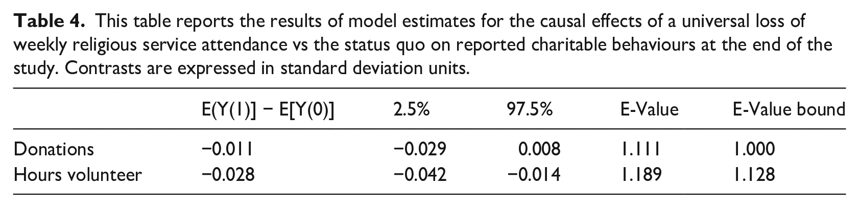
For donations, the effect estimate is −0.011 [−0.029, 0.008]. The E-value for this estimate is 1.111, with a lower bound of 1. We infer that the evidence for causality is not reliable. On the data scale, this intervention represents a difference of NZD −54.72 per adult per year in charitable giving compared to the status quo. Still, again, this effect is not reliable.

The effect estimate for hours volunteered is −0.028 [−0.042, −0.014]. The E-value for this estimate is 1.189, with a lower bound of 1.128. We infer evidence for causality. On the data scale, this intervention represents a difference of −6.88 in volunteering minutes compared with the status quo.

Study 2: Causal effects of regular Church attendance on support received from others – time

Regular vs zero causal treatment contrast for time received from others

Figure 4(a) and Table 5 present results for the treatment contrasts between regular religious attendance and zero, focusing on voluntary help received from others during the past week (yes/no). These results are estimated on the risk ratio scale.

Figure 4.

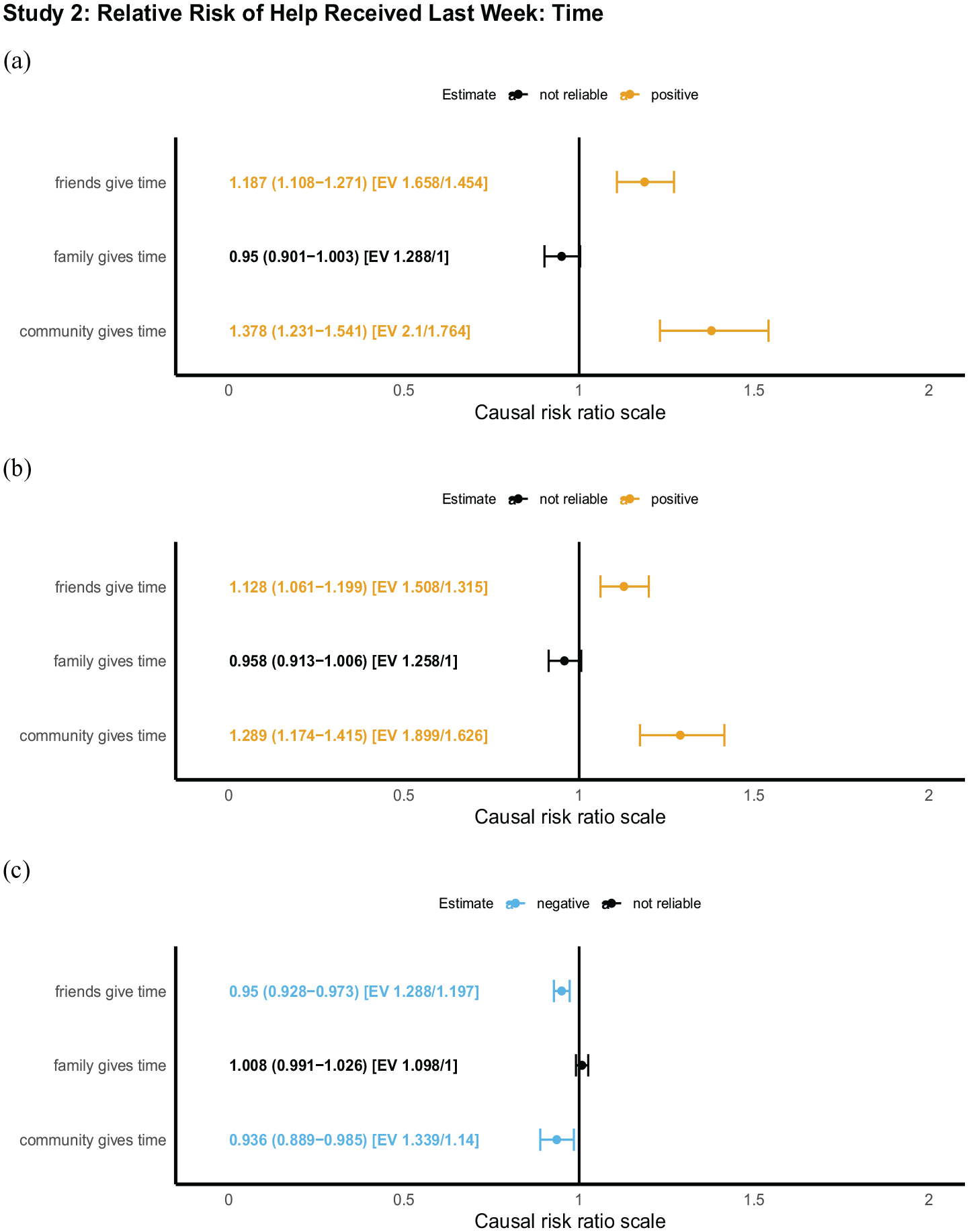
This figure reports the results of model estimates for the three causal contrasts of interest on help received from others during the past week (yes/no). The causal contrasts are (a) Regular vs Zero Religious Service Attendance, (b) Regular Religious Service Attendance vs Status Quo, and (c) Zero Religious Service Attendance vs Status Quo. Contrasts are expressed on the risk ratio scale.

Table 5.

This table reports the results of model estimates for the causal effects of a universal gain of weekly religious attendance vs a universal loss of weekly religious attendance on voluntary help received from others during the past week (yes/no) at the end of the study. Contrasts are expressed on the risk ratio scale.

	E(Y(1)]/E[Y(0)]	2.5%	97.5%	E-Value	E-Value bound
Family gives time	0.950	0.901	1.003	1.288	1.000
Friends give time	1.187	1.108	1.271	1.658	1.454
Community gives time	1.378	1.231	1.541	2.100	1.764

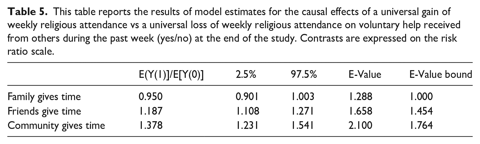
For community gives time, the effect estimate is 1.378 [1.231, 1.541]. The E-value for this estimate is 2.1, with a lower bound of 1.764. At this lower bound, unmeasured confounders would need a minimum association strength with both the intervention sequence and outcome of 1.764 to negate the observed effect. Weaker confounding would not overturn it. We infer evidence for causality.

For friends give time, the effect estimate is 1.187 [1.108, 1.271]. The E-value for this estimate is 1.658, with a lower bound of 1.454. We infer evidence for causality.

For family gives time, the effect estimate is 0.95 [0.901, 1.003]. The E-value for this estimate is 1.288, with a lower bound of 1. We infer that evidence for causality is not reliable.

Regular religious service vs status quo treatment contrast for time received from others

Figure 4(b) and Table 6 present results for the treatment contrasts between regular religious service and status quo, focusing on voluntary help received from others during the past week (yes/no). These results are again estimated on the risk ratio scale.

Table 6.

This table reports the results of model estimates for the causal effects of a universal gain of weekly religious attendance vs the status quo on voluntary help received from others during the past week (yes/no) at the end of the study. Contrasts are expressed on the risk ratio scale.

	E(Y(1)]/E[Y(0)]	2.5%	97.5%	E-Value	E-Value bound
Family gives time	0.958	0.913	1.006	1.258	1.000
Friends give time	1.128	1.061	1.199	1.508	1.315
Community gives time	1.289	1.174	1.415	1.899	1.626

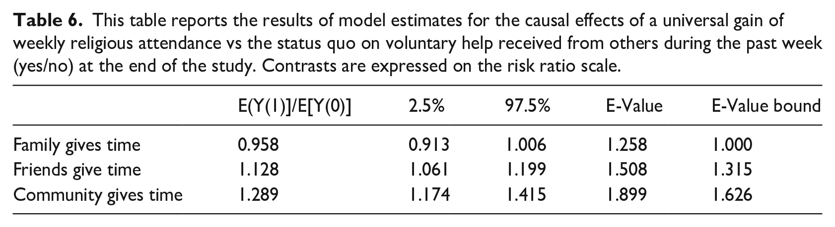
For community gives time, the effect estimate is 1.289 [1.174, 1.415]. The E-value for this estimate is 1.899, with a lower bound of 1.626. At this lower bound, unmeasured confounders would need a minimum association strength with both the intervention sequence and outcome of 1.626 to negate the observed effect. Weaker confounding would not overturn it. We infer evidence for causality.

For friends give time, the effect estimate is 1.128 [1.061, 1.199]. The E-value for this estimate is 1.508, with a lower bound of 1.315. We infer evidence for causality.

For family gives time, the effect estimate is 0.958 [0.913, 1.006]. The E-value for this estimate is 1.258, with a lower bound of 1. We infer that evidence for causality is not reliable.

Zero religious service vs status quo treatment contrast for time received from others

Figure 4(c) and Table 7 present results for the treatment contrasts between zero religious service and status quo, focusing on voluntary help received from others during the past week (yes/no). These causal effect estimates are again expressed on the risk ratio scale.

Table 7.

This table reports results of model estimates for the causal effects of a universal loss of weekly religious service attendance vs the status quo on voluntary help received from others during the past week (yes/no) at the end of the study. Contrasts are expressed on the risk ratio scale.

	E(Y(1)]/E[Y(0)]	2.5%	97.5%	E-Value	E-Value bound
Family gives time	1.008	0.991	1.026	1.098	1.000
Friends give time	0.950	0.928	0.973	1.288	1.197
Community gives time	0.936	0.889	0.985	1.339	1.140

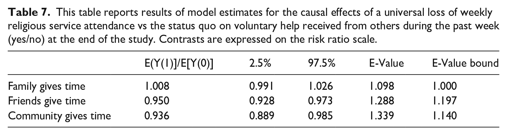
For family gives time, the effect estimate is 1.008 [0.991, 1.026]. The E-value for this estimate is 1.098, with a lower bound of 1. We infer that evidence for causality is not reliable.

For friends give time, the effect estimate is 0.95 [0.928, 0.973]. The E-value for this estimate is 1.288, with a lower bound of 1.197. At this lower bound, unmeasured confounders would need a minimum association strength with both the intervention sequence and outcome of 1.197 to negate the observed effect. We infer evidence for causality.

For community gives time, the effect estimate is 0.936 [0.889, 0.985]. The E-value for this estimate is 1.339, with a lower bound of 1.14. We infer evidence for causality.

Study 3: causal effects of regular Church attendance on support received from others – money

Regular vs zero causal contrast on money received from others

Figure 5(a) and Table 8 present results for the treatment contrasts between regular religious service and zero, focusing on money received from others during the past week (yes/no). These results are again presented on the risk ratio scale.

Figure 5.

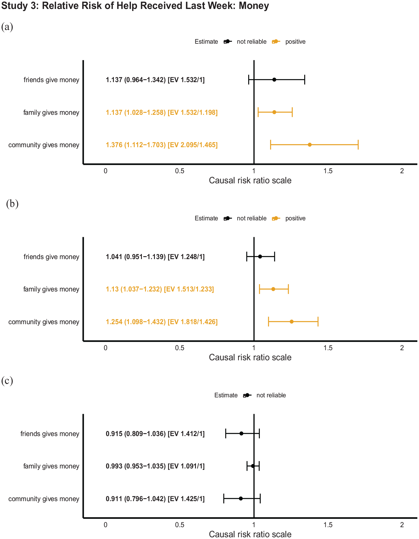
This figure reports the results of model estimates for the three causal contrasts of interest on help received from others during the past week (yes/no). The causal contrasts are: (a) Regular vs Zero Religious Service Attendance (b) Regular Religious Service Attendance vs Status Quo; (b) Zero Religious Service Attendance vs Status Quo. Contrasts are expressed on the risk ratio scale.

Table 8.

This table reports the results of model estimates for the causal effects of a universal gain of weekly religious service vs a universal loss of weekly religious service on financial help received from others during the past week (yes/no) at the end of the study. Contrasts are expressed on the risk ratio scale.

	E(Y(1)]/E[Y(0)]	2.5%	97.5%	E-Value	E-Value bound
Family gives money	1.137	1.028	1.258	1.532	1.198
Friends give money	1.137	0.964	1.342	1.532	1.000
Community gives money	1.376	1.112	1.703	2.095	1.465

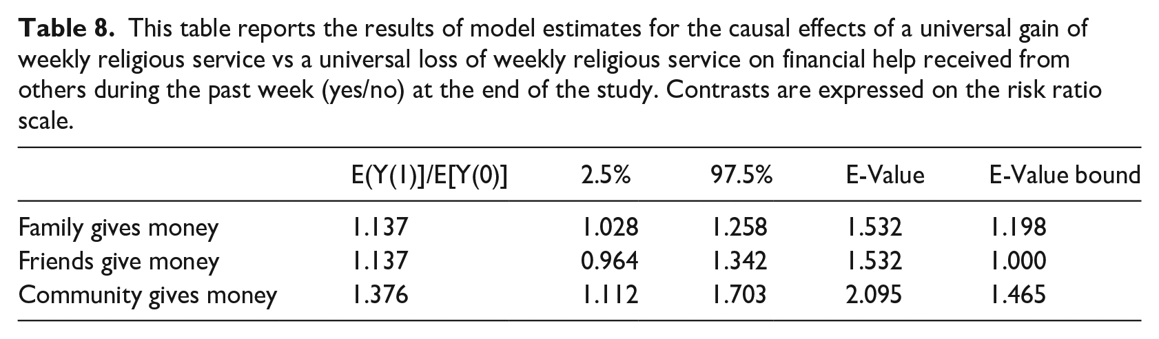
For community gives money, the effect estimate is 1.376 [1.112, 1.703]. The E-value for this estimate is 2.095, with a lower bound of 1.465. At this lower bound, unmeasured confounders would need a minimum association strength with both the intervention sequence and outcome of 1.465 to negate the observed effect. We infer evidence for causality.

For family gives money, the effect estimate is 1.137 [1.028, 1.258]. The E-value for this estimate is 1.532, with a lower bound of 1.198. We infer evidence for causality.

For friends gives money, the effect estimate is 1.137 [0.964, 1.342]. The E-value for this estimate is 1.532, with a lower bound of 1. We infer that evidence for causality is not reliable.

Regular vs status quo causal contrast on money received from others

Figure 5(b) and Table 9 present results for the treatment contrasts between regular religious service and status quo, focusing on money received from others during the past week (yes/no). These results are expressed on the risk ratio scale.

Table 9.

This table reports the results of model estimates for the causal effects of a universal gain of weekly religious service vs the status quo on financial help received from others during the past week (yes/no) at the end of the study. Contrasts are expressed on the risk ratio scale.

	E(Y(1)]/E[Y(0)]	2.5%	97.5%	E-Value	E-Value bound
Family gives money	1.130	1.037	1.232	1.513	1.233
Friends give money	1.041	0.951	1.139	1.248	1.000
Community gives money	1.254	1.098	1.432	1.818	1.426

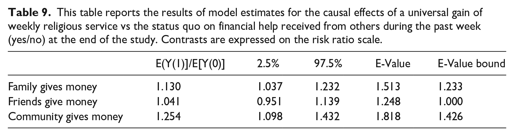
For community gives money, the effect estimate is 1.254 [1.098, 1.432]. The E-value for this estimate is 1.818, with a lower bound of 1.426. At this lower bound, unmeasured confounders would need a minimum association strength with both the intervention sequence and outcome of 1.426 to negate the observed effect. Weaker confounding would not overturn it. We infer evidence for causality.

For family gives money, the effect estimate is 1.13 [1.037, 1.232]. The E-value for this estimate is 1.513, with a lower bound of 1.233. At this lower bound, unmeasured confounders would need a minimum association strength with both the intervention sequence and outcome of 1.233 to negate the observed effect. We infer evidence for causality.

For friends gives money, the effect estimate is 1.041 [0.951, 1.139]. The E-value for this estimate is 1.248, with a lower bound of 1. We infer that evidence for causality is not reliable.

Zero vs status quo causal contrast on money received from others

Figure 5(c) and Table 10 present results for the treatment contrasts between zero religious service and status quo, focusing on money received from others during the past week (yes/no). These results are expressed on the risk ratio scale.

Table 10.

Table reports results of model estimates for the causal effects of a universal loss of weekly religious service vs the status quo on financial help received from others during the past week (yes/no) at the end of study. Contrasts are expressed on the risk ratio scale.

	E(Y(1)]/E[Y(0)]	2.5%	97.5%	E-Value	E-Value bound
Family gives money	0.993	0.953	1.035	1.091	1
Friends gives money	0.915	0.809	1.036	1.412	1
Community gives money	0.911	0.796	1.042	1.425	1

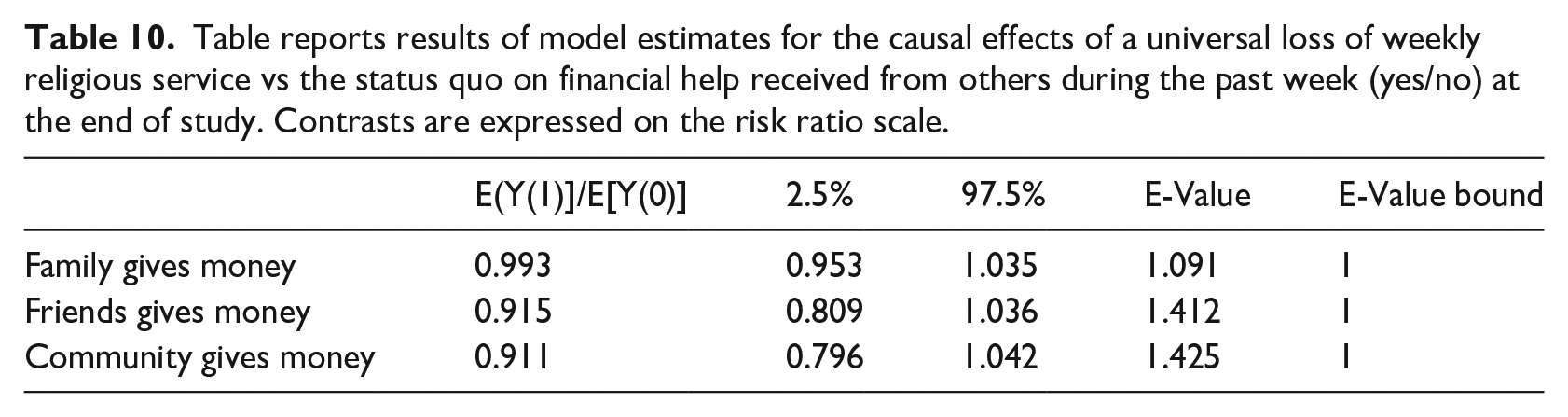
For family gives money, the effect estimate on the risk ratio scale is 0.993 [0.953, 1.035]. The E-value for this estimate is 1.091, with a lower bound of 1. We infer that evidence for causality is not reliable.

For friends gives money, the effect estimate on the risk ratio scale is 0.915 [0.809, 1.036]. The E-value for this estimate is 1.412, with a lower bound of 1. We infer that evidence for causality is not reliable.

For community gives money, the effect estimate on the risk ratio scale is 0.911 [0.796, 1.042]. The E-value for this estimate is 1.425, with a lower bound of 1. We infer that evidence for causality is not reliable.

Additional study: comparison of causal inference results with cross-sectional regressions

To clarify how our causal inferences compare with estimates from commonly used observational research methods, we quantified the statistical associations between religious service attendance and all prosocial outcomes using cross-sectional methods frequently employed in observational psychology. For each analysis, we included all regression covariates from the causal models, including sample weights, while omitting the baseline measurement of the outcome variable.

Cross-sectional volunteering result

The change in expected hours of volunteer work for a one-unit increase in religious service attendance is b = 0.31; (95% confidence interval (CI): 0.28, 0.34). Multiplying this by 4.2 gives a monthly estimate of 77.95 minutes. This result is 2.58% greater than the effect estimated from the ‘regular vs zero’ causal contrast, revealing an overstatement in the cross-sectional regression model.

Cross-sectional charitable donations result

The coefficient for religious service on annual charitable donations suggests a change in expected donation amount per unit increase in attendance is b = 451; (95% CI: 408, 494). When adjusted to a monthly rate by multiplying by 4.2, this value equals NZ Dollars 1894.45. It is 2.89% greater than our causal contrast estimate, again revealing an overstatement in the cross-sectional regression model.

For Studies 2 and 3, which focus on community help received, we handled the non-collapsibility of odds ratios by assuming a Poisson distribution for the outcome variables, and thus obtaining a rate ratio that approximates a risk ratio (Huitfeldt et al., 2019; VanderWeele et al., 2020).

Cross-sectional community assistance received result: Time

The exponentiated change in expectation for a one-unit change in religious service attendance is b = 1.17; (95% CI: 1.14, 1.19) approximate risk rate ratio. The monthly rate ratio derived by multiplying this coefficient by 4.2 is 1.921. This estimate is 1.39% greater than the ‘regular vs zero’ causal estimate, revealing an overstatement of effect-estimate from that the cross-sectional regression model suggests.

Cross-sectional community assistance received result: Money

Similarly, the exponentiated change for money received yields an approximate risk ratio of b = 1.18; (95% CI: 1.08, 1.27). The monthly risk ratio, after adjustment, is 1.996. This rate ratio is 1.45% greater than the causal estimate, again revealing an overstatement in the cross-sectional regression model.

These findings indicate that while cross-sectional regression results may be suggestive, they can differ substantially from those obtained through the causal analysis of panel data.

Economic effects of religious service attendance on charitable donations

We next use our results to estimate the approximate economic value of religious service attendance under different scenarios—‘Regular Religious Service Attendance’, ‘Zero Religious Service Attendance’, and the ‘status quo’, focusing on charitable donations. We find the expected total donations under the interventions we modelled are as follows:

Regular Religious Service: an increase in religious service attendance yields an individual average donation sum of NZD 1638.98.

Zero Religious Service: Reducing religious service attendance to zero yields an average donation sum of NZD 984.59.

Status Quo: The expected individual average donation sum is currently NZD 1037.14.

With 3,989,000 adult residents in New Zealand in 2021.¹ We find that:

First, multiplying the adult population by the average donation sum gives a status quo national estimate for charitable giving of NZD 4,137,151,460.

Second, the net gain to charity from country-wide regular attendance at religious services, compared to the status quo, is NZD 2,400,739,760.

Third, although the net cost to charity from a complete cessation of regular religious service attendance is NZD −209,621,950, recall the confidence interval crosses zero, and this effect is not reliable.

To provide context, we next consider the magnitude of these economic consequences by comparing them to the New Zealand government’s annual budget. In the year the outcomes were measured (2021–2022), this budget amounted to NZD 57,976,000,000.

First, the expected gain from a nationwide adoption of regular religious service represents 4.1% of New Zealand’s annual government budget 2021.

Second, we do not find a reliable one-year effect on charitable giving from the loss intervention.

Hence, the scenario in which all New Zealand adults were to regularly attend religious services implies a substantial increase in society-wide charitable support one year after the intervention compared to the status quo. On the contrary, the scenario in which New Zealand was to experience a complete cessation of religious service attendance is not reliably distinguishable from the status quo condition.

We emphasise that these population-wide estimates for aggregated one-year effects following interventions reflect short-term behavioural changes. They do not account for the longer-term implications of gaining or losing religious institutions on charity and volunteering.

Discussion

Our study provides causal evidence that adopting regular religious service attendance across New Zealand would increase levels of charity and volunteering. On the other hand, results also suggest that completely eliminating religious services would produce relatively minor changes in the year following cessation – a finding attributable to low baseline levels of religious attendance.

This study underscores the importance of careful causal inquiry for examining the social consequences of religion. The broad question, ‘Does religion cause prosociality?’ is too vague to yield meaningful insights. Effective investigation requires specifying causal contrasts with well-defined treatments, selecting relevant measures of religious belief and behaviour, defining the target population, and collecting appropriate repeated-measures data in sufficiently large samples over time. Furthermore, only after satisfying fundamental causal assumptions and identification criteria can we derive reliable statistical estimates that address our research questions. Employing flexible statistical estimators further mitigates the risk of model misspecification (Hoffman et al., 2023; Van der Laan & Rose, 2018; Wager & Athey, 2018). Following statistical estimation, sensitivity analyses are essential to assess the robustness of our quantitative estimates to confounding bias (Hernan & Robins, 2024; VanderWeele et al., 2020).

In this study, we defined clear causal contrasts based on interventions that either increased or decreased religious service attendance, or maintained attendance at the status quo. Our statistical models accounted for baseline confounders, including measures of baseline treatment and baseline outcomes. To minimise reliance on modelling assumptions, we employed flexible, doubly robust machine learning ensembles with cross-validation. We then compared expected average outcomes under different treatments one year after the interventions, ensuring that estimation adhered to a temporal order in which causes precede effects.

We introduced two novel measures of prosociality – help received and financial support from one’s community. Although these indicators may be subject to measurement error, they help mitigate concerns related to self-presentation bias, as few would boast of dependency. Findings from these indicators cooberate the findings we obtain from self-reported charitable donations and volunteering, lending support to evolutionary theories of religious prosociality, which propose that a fundamental, evolved function of religion is to enhance community-making (Sosis & Bressler, 2003; Watts et al., 2015, 2018; Whitehouse et al., 2023).

Importantly, our findings suggest that traditional effect size measures, such as Cohen’s d or $R^{2}$ , can misrepresent practical significance when not grounded in causal inference. Specifically, the concept of an ‘effect size’ makes is less meaningful for a mere statistical association absent a consistently estimated causal effect. For instance, although the standardised effect size for the contrast between regular and zero religious service attendance is modest (0.132 (0.102, 0.161)), this corresponds to an increase in annual charitable donations from NZD 1037.14 to NZD 1638.98 per individual. This expected increase amounts to 4% of New Zealand’s 2021 government budget – a substantial real-world impact. This finding illustrates the limitations of relying on conventional statistical measures without considering valid causal estimates, particularly when informing policy. We recommend that researchers prioritise causal inference to evaluate and communicate practical effect sizes.

An intriguing question remains: who benefits from the charity of religious individuals? Although our data indicate that religious individuals often receive help from their communities, it is unclear whether those providing the help are members of the same religious group. For instance, religious service attendance might increase requests for assistance – begging – which non-religious community members could then fulfill. Similarly, religious giving and volunteering might disproportionately benefit religious elites, potentially at the expense of broader public goods. Although these scenarios may seem extreme, our data do not exclude them because our data do not describe the network structure of charitable giving. Nevertheless, we may look to other data sources for insights.

In New Zealand, religious organisations operate as public charities with transparent financial records. Public data show that religious institutions account for 40% of the charitable sector in New Zealand (McLeod, 2020 p. 17), with similar or even higher proportions observed in other countries (Brooks, 2004; Monsma, 2007; Woodyard & Grable, 2014). Furthermore, evidence suggests that religious organisations are efficient charities with low administrative costs and high volunteer engagement (Bekkers & Wiepking, 2011b; Khanna et al., 1995; McLeod, 2020 p. 26). Of course, we cannot dismiss the possibility that some religious leaders pocket a large share of benefits from religious charities. However, given that all charities in New Zealand require open books, with published institutional salaries and legal punishments for theft, such instances are presumably rare. Secular charities, or course, are not immune to corruption. Measurement error poses a threat. However, whether this threat is upwardly biased to favour religion-based charity and volunteering remains uncertain. Based on contextual information, it seems credible to speculate that most religious charity goes to genuinely charitable causes. Nevertheless, we reiterate that our data do not address this question.

Despite the strengths of our study, several limitations persist. It is important not to confuse the precision of our causal workflow with the precision of the estimates that we derive from it. Direct and correlated measurement errors can skew findings by inflating or reducing estimated magnitudes of true effects (Bulbulia, 2024d; VanderWeele & Hernán, 2012). As noted by Bekkers and Wiepking (2011a), even uncorrelated errors can distort estimates of charitable giving, leading to downward biases in religious charity estimates. Although we employed multiple measures and adjusted for baseline giving to reduce the effects of systematic errors, measurement errors may nevertheless influence our results. For instance, our models might underestimate the true costs of religious decline in the near term. Since religious institutions comprise 40% of New Zealand’s charitable sector, a significant drop in religious attendance could threaten the viability of these charities. Put differently, our one-year estimates of charitable giving and volunteering may present a false picture of security. Conversely, a sharp rise in religious attendance might yield more considerable benefits than our models suggest. We do not claim to possess a magical crystal ball; our results offer signals, not certainties.

The generalisability of our findings beyond New Zealand is yet to be examined. Although our results pertain to the New Zealand population, further research is necessary to determine whether they hold in other cultural or national contexts. Initiatives such as the Global Flourish Study (B. R. Johnson & VanderWeele, 2022), and similar efforts will eventually provide opportunities to apply causal methods across diverse cultural settings. Also remaining to be investigated are the causal effects on prosociality of prolonged exposure to religious services over many years, another fascinating horizon for future investigations.

In conclusion, by integrating robust causal methods with longitudinal data, we provide clear quantitative evidence that religious service attendance influences prosocial behaviours. Beyond the significance of our findings, we hope this study encourages psychological scientists to adopt causal methods in their research. Psychological questions are inherently causal; however, effectively addressing these questions requires careful causal methods that differ from the associational approaches that currently dominate teaching and research (Bulbulia, 2024e; Rohrer et al., 2022; VanderWeele, 2021). We hope this study inspires others to build upon this early effort to ask, and answer, clearly defined causal questions about the causal effects of religious service attendance on charity and volunteering.

Supplemental Material

sj-docx-1-prj-10.1177_00846724241302810 – Supplemental material for The causal effects of religious service attendance on prosocial behaviours in New Zealand: A national longitudinal study

Supplemental material, sj-docx-1-prj-10.1177_00846724241302810 for The causal effects of religious service attendance on prosocial behaviours in New Zealand: A national longitudinal study by Joseph A Bulbulia, Don E Davis, Kenneth G Rice, Chris G Sibley and Geoffrey Troughton in Archive for the Psychology of Religion/Archiv Für Religionpsychologie

Footnotes

Author contribution

J.B. conceived the study and approach and wrote the draft manuscript. C.S. led NZAVS data collection. All authors contributed to the manuscript.

Data availability

The data described in the paper are part of the New Zealand Attitudes and Values Study. Members of the NZAVS management team and research group hold full copies of the NZAVS data. A de-identified dataset containing only the variables analysed in this manuscript is available upon request from the corresponding author or any member of the NZAVS advisory board for replication or checking of any published study using NZAVS data. The code for the analysis can be found at: .

Funding

The author(s) disclosed receipt of the following financial support for the research, authorship, and/or publication of this article: The New Zealand Attitudes and Values Study is supported by a grant from the Templeton Religious Trust (grant nos. TRT0196 and TRT0418). J.B. received support from the Max Planck Institute for the Science of Human History. The funders had no role in preparing the manuscript or deciding to publish it.

Ethical approval

The University of Auckland Human Participants Ethics Committee reviews the NZAVS every 3 years. Our most recent ethics approval statement is as follows: The New Zealand Attitudes and Values Study was approved by the University of Auckland Human Participants Ethics Committee on 26 May 2021 for 6 years until 26 May 2027 (ref. no. UAHPEC22576).

ORCID iD

Joseph A Bulbulia

Kenneth Rice

Geoffrey Troughton

Supplemental material

Supplemental material for this article is available online: .

Notes

References

Bekkers

Wiepking

(2011a). Accuracy of self-reports on donations to charitable organizations. Quality & Quantity, 45, 1369–1383.

Bekkers

Wiepking

(2011b). A literature review of empirical studies of philanthropy: Eight mechanisms that drive charitable giving. Nonprofit and Voluntary Sector Quarterly, 40(5), 924–973.

Brooks

A. C.

(2004). Faith, secularism, and charity. Faith & Economics, 43(Spring), 1–8.

Bulbulia

J. A.

(2024a). Margot: MARGinal observational treatment-effects. https://doi.org/10.5281/zenodo.10907724

Bulbulia

J. A.

(2024b). Methods in causal inference part 1: Causal diagrams and confounding. Evolutionary Human Sciences, 6, Article e40. https://doi.org/10.1017/ehs.2024.35

Bulbulia

J. A.

(2024c). Methods in causal inference part 2: Interaction, mediation, and time-varying treatments. Evolutionary Human Sciences, 6, Article e41. https://doi.org/10.1017/ehs.2024.32

Bulbulia

J. A.

(2024d). Methods in causal inference part 3: Measurement error and external validity threats. Evolutionary Human Sciences, 6, Article e42. https://doi.org/10.1017/ehs.2024.33

Bulbulia

J. A.

(2024e). A practical guide to causal inference in three-wave panel studies. PsyArXiv Preprints. https://doi.org/10.31234/osf.io/uyg3d

Chatton

Le Borgne

Leyrat

Gillaizeau

Rousseau

Barbin

Laplaud

Léger

Giraudeau

Foucher

(2020). G-computation, propensity score-based methods, and targeted maximum likelihood estimator for causal inference with different covariates sets: A comparative simulation study. Scientific Reports, 10(1), 9219. https://doi.org/10.1038/s41598-020-65917-x

10.

Chen

Benesty

. . .Yuan

(2023). Xgboost: Extreme gradient boosting. https://CRAN.R-project.org/package=xgboost

11.

Danaei

Tavakkoli

Hernán

M. A.

(2012). Bias in observational studies of prevalent users: Lessons for comparative effectiveness research from a meta-analysis of statins. American Journal of Epidemiology, 175(4), 250–262. https://doi.org/10.1093/aje/kwr301

12.

De Coulanges

. (1903). The ancient city: A study on the religion, laws, and institutions of Greece and Rome (W. Small, Trans.). Lee and Shepard. (Original work published 1864).

13.

Díaz

Williams

Hoffman

K. L.

Schenck

E. J.

(2023). Nonparametric causal effects based on longitudinal modified treatment policies. Journal of the American Statistical Association, 118(542), 846–857. https://doi.org/10.1080/01621459.2021.1955691

14.

Haneuse

Rotnitzky

(2013). Estimation of the effect of interventions that modify the received treatment. Statistics in Medicine, 32(30), 5260–5277.

15.

Hernán

M. A.

Greenland

(2024). Why stating hypotheses in grant applications is unnecessary. Journal of the American Medical Association, 331(4), 285–286.

16.

Hernan

M. A.

Robins

J. M.

(2024). Causal inference: What if? https://www.hsph.harvard.edu/miguel-hernan/causal-inference-book/

17.

Hernán

M. A.

Sauer

B. C.

Hernández-Díaz

Platt

Shrier

(2016). Specifying a target trial prevents immortal time bias and other self-inflicted injuries in observational analyses. Journal of Clinical Epidemiology, 79, 70–75.

18.

Hoffman

K. L.

Salazar-Barreto

Rudolph

K. E.

Díaz

(2023). Introducing longitudinal modified treatment policies: A unified framework for studying complex exposures. https://doi.org/10.48550/arXiv.2304.09460

19.

Huitfeldt

Stensrud

M. J.

Suzuki

(2019). On the collapsibility of measures of effect in the counterfactual causal framework. Emerging Themes in Epidemiology, 16, 1–5.

20.

Johnson

B. R.

VanderWeele

T. J.

(2022). The global flourishing study: A new era for the study of well-being. International Bulletin of Mission Research, 46(2), 272–275.

21.

Johnson

D. D.

(2005). God’s punishment and public goods: A test of the supernatural punishment hypothesis in 186 world cultures. Human Nature, 16, 410–446.

22.

Kelly

J. M.

Kramer

S. R.

Shariff

A. F.

(2024). Religiosity predicts prosociality, especially when measured by self-report: A meta-analysis of almost 60 years of research. Psychological Bulletin, 150(3), 284–318.

23.

Khanna

Posnett

Sandler

(1995). Charity donations in the UK: New evidence based on panel data. Journal of Public Economics, 56(2), 257–272.

24.

Linden

Mathur

M. B.

VanderWeele

T. J.

(2020). Conducting sensitivity analysis for unmeasured confounding in observational studies using e-values: The evalue package. The Stata Journal, 20(1), 162–175.

25.

Major-Smith

(2023). Exploring causality from observational data: An example assessing whether religiosity promotes cooperation. Evolutionary Human Sciences, 5, Article e22.

26.

McLeod

(2020). The New Zealand Support Report: The current state and significance of giving in New Zealand and the outlook for recipients. JBWere. https://www.jbwere.co.nz/media/1qudxw3q/jbwere-nz-support-report-digital.pdf

27.

Monsma

S. V.

(2007). Religion and philanthropic giving and volunteering: Building blocks for civic responsibility. Interdisciplinary Journal of Research on Religion, 3, 2–28.

28.

Norenzayan

Shariff

A. F.

Gervais

W. M.

Willard

A. K.

McNamara

R. A.

Slingerland

Henrich

(2016). The cultural evolution of prosocial religions. Behavioral and Brain Sciences, 39, Article e1. https://doi.org/10.1017/S0140525X14001356

29.

Polley

LeDell

Kennedy

Van der Laan

(2023). SuperLearner: Super learner prediction. https://CRAN.R-project.org/package=SuperLearner

30.

Rohrer

J. M.

Hünermund

Arslan

R. C.

Elson

(2022). That’s a lot to process! Pitfalls of popular path models. Advances in Methods and Practices in Psychological Science, 5(2), 25152459221095827. https://doi.org/10.1177/25152459221095827

31.

Schloss

J. P.

Murray

M. J.

(2011). Evolutionary accounts of belief in supernatural punishment: A critical review. Religion, Brain & Behavior, 1(1), 46–99.

32.

Sibley

C. G.

(2021). Sampling procedure and sample details for the New Zealand Attitudes and Values Study. https://osf.io/preprints/psyarxiv/wgqvy

33.

Sosis

Bressler

E. R.

(2003). Cooperation and commune longevity: A test of the costly signaling theory of religion. Cross-cultural Research, 37(2), 211–239.

34.

Suzuki

Shinozaki

Yamamoto

(2020). Causal diagrams: Pitfalls and tips. Journal of Epidemiology, 30(4), 153–162. https://doi.org/10.2188/jea.JE20190192

35.

Swanson

G. E.

(1967). Religion and regime: A sociological account of the reformation. https://academic.oup.com/psq/article-pdf/85/1/129/51268754/psquar_85_1_129.pdf

36.

Van Buuren

. (2018). Flexible imputation of missing data. CRC Press.

37.

Van der Laan

M. J

. (2014). Targeted estimation of nuisance parameters to obtain valid statistical inference. The International Journal of Biostatistics, 10(1), 29–57.

38.

Van der Laan

M. J.

Gruber

. (2012). Targeted minimum loss based estimation of causal effects of multiple time point interventions. The International Journal of Biostatistics, 8(1), 1370.

39.

Van der Laan

M. J.

Rose

. (2018). Targeted learning in data science: Causal inference for complex longitudinal studies. Springer. http://link.springer.com/10.1007/978-3-319-65304-4

40.

VanderWeele

T. J.

(2009). Concerning the consistency assumption in causal inference. Epidemiology, 20(6), 880. https://doi.org/10.1097/EDE.0b013e3181bd5638

41.

VanderWeele

T. J.

(2019). Principles of confounder selection. European Journal of Epidemiology, 34(3), 211–219.

42.

VanderWeele

T. J.

(2021). Can sophisticated study designs with regression analyses of observational data provide causal inferences? JAMA Psychiatry, 78(3), 244–246.

43.

VanderWeele

T. J.

Ding

(2017). Sensitivity analysis in observational research: Introducing the E-value. Annals of Internal Medicine, 167(4), 268–274. https://doi.org/10.7326/M16-2607

44.

VanderWeele

T. J.

Hernán

M. A.

(2012). Results on differential and dependent measurement error of the exposure and the outcome using signed directed acyclic graphs. American Journal of Epidemiology, 175(12), 1303–1310. https://doi.org/10.1093/aje/kwr458

45.

VanderWeele

T. J.

Hernan

M. A.

(2013). Causal inference under multiple versions of treatment. Journal of Causal Inference, 1(1), 1–20.

46.

VanderWeele

T. J.

Mathur

M. B.

Chen

(2020). Outcome-wide longitudinal designs for causal inference: A new template for empirical studies. Statistical Science, 35(3), 437–466.

47.

Wager

Athey

(2018). Estimation and inference of heterogeneous treatment effects using random forests. Journal of the American Statistical Association, 113(523), 1228–1242. https://doi.org/10.1080/01621459.2017.1319839

48.

Watts

Bulbulia

J. A.

Gray

R. D.

Atkinson

Q. D.

(2016). Clarity and causality needed in claims about big gods. Behavioral and Brain Sciences, 39, 41–42. https://doi.org/10.1017/S0140525X15000576

49.

Watts

Greenhill

S. J.

Atkinson

Q. D.

Currie

T. E.

Bulbulia

Gray

R. D.

(2015). Broad supernatural punishment but not moralizing high gods precede the evolution of political complexity in Austronesia. Proceedings of the Royal Society B: Biological Sciences, 282, 20142556.

50.

Watts

Sheehan

Bulbulia Joseph

Gray

R. D.

Atkinson

Q. D.

(2018). Christianity spread faster in small, politically structured societies. Nature Human Behaviour, 2(8), 559–564. https://doi.org/10/gdvnjn

51.

Westreich

Cole

S. R.

(2010). Invited commentary: Positivity in practice. American Journal of Epidemiology, 171(6), 674–677. https://doi.org/10.1093/aje/kwp436

52.

Wheatley

(1971). The pivot of the four quarters: A preliminary enquiry into the origins and character of the ancient Chinese City. Edinburgh University Press. https://cir.nii.ac.jp/crid/1130000795717727104

53.

Whitehouse

Francois

Savage

P. E.

Turchin

(2023). Testing the big gods hypothesis with global historical data: A review and retake. Religion, Brain & Behavior, 13(2), 124–166.

54.

Williams

N. T.

Díaz

(2021). lmtp: Non-parametric causal effects of feasible interventions based on modified treatment policies. https://doi.org/10.5281/zenodo.3874931

55.

Woodyard

Grable

(2014). Doing good and feeling well: Exploring the relationship between charitable activity and perceived personal wellness. VOLUNTAS: International Journal of Voluntary and Nonprofit Organizations, 25, 905–928.

56.

Wright

M. N.

Ziegler

(2017). Ranger: A fast implementation of random forests for high dimensional data in C++ and R. Journal of Statistical Software, 77(1), 1–17. https://doi.org/10.18637/jss.v077.i01

57.

Zhang

Dashti

S. G.

Carlin

J. B.

Lee

K. J.

Moreno-Betancur

(2023). Should multiple imputation be stratified by exposure group when estimating causal effects via outcome regression in observational studies? BMC Medical Research Methodology, 23(1), 42.

Supplementary Material

Please find the following supplemental material available below.

For Open Access articles published under a Creative Commons License, all supplemental material carries the same license as the article it is associated with.

For non-Open Access articles published, all supplemental material carries a non-exclusive license, and permission requests for re-use of supplemental material or any part of supplemental material shall be sent directly to the copyright owner as specified in the copyright notice associated with the article.

0.00 MB

0.20 MB