Sage Journals: Discover world-class research

Abstract

Because of the non-uniformity of the CIELAB color space, scientists and researchers have tried to find the best formula for the CIELAB color space which provides consistent color difference results. The computing performances of the four color difference formulas (CIELAB1976, CMC, CIE94, and CIEDE2000) were tested in the four principal hue regions of the CIELAB color space at a constant lightness value of 50 (L* = 50) which corresponds to the largest chromaticity plane around the gray point (L* = 50; a* = 0; b* = 0). The dependence and consistency of the four formulas were investigated according to regular and constant color coordinate changes by using a specially prepared computer software. The experimental results showed that the three formulas other than CIELAB1976 computed in different manners peculiar to themselves and the CMC formula gave the most distinct results on different hue regions of the a*–b* color plane. CIELAB1976, CIE94, and CIEDE2000 formulas were found to compute the most consistent color difference results in the different hue regions. The color difference (ΔE*) computing behaviors of the three formulas, other than CIELAB1976, changed depending on hue and chroma differences due to polar color difference considerations of their formulas, as expected.

Keywords

CIELAB color difference CIELAB1976 CMC CIE94 CIEDE2000 hue chroma color plane

CIELAB color space was defined in 1976 by Commission Internationale de l’Eclairage (CIE; International Commission on Illumination) after extensive research to find a visually uniform color space which will be consistent with the visual and computing results. In addition, two different color difference equations (formulas), i.e., CIELAB (1976) and CIELCh (1976), were proposed. The CIELAB color space was characterized in Cartesian coordinates by three independent axes. The three axes presented lightness (L*), red–green (a*), and yellow–blue (b*) coordinates, placing the lightness axis as the main factor. The further color-related terms of chroma (C*) and hue angle (h) were also computed by their coordinate-dependent formulas.¹ The fingerprints of visual colors are tristimulus values (X, Y, and Z) in addition to their percentage reflectance-wavelength curves. They are measured and calculated under specified illumination and viewing conditions by the inclusion of reflectance values obtained at predetermined wavelengths according to the diode capacity and capability of the color-measuring instruments, i.e., reflectance spectrophotometers, at 10- or 20-nm intervals.^1,2

The defined color difference equations, CIELAB (1976) (or CIELAB1976; CIEL*a*b*) and CIELCh (1976) were formulated to calculate the color difference (ΔE*) between two color points in the color space, one being the reference (target) and the other being a sample color. However, soon after 1976, it was found that CIELAB color space was not visually uniform. This finding meant that equal calculated color difference magnitudes (Euclidean distance) did not correspond with equal visual differences. In other words, equal numerical color differences did not correspond with equal visual differences. In addition, the magnitude of the differences varied in different parts of the CIELAB color space. This meant that a ΔE* value obtained by say the CIELAB (1976) equation corresponded to a visual color difference in one part of the space but the same numerical ΔE* did not correspond to a visual difference in another part of the space. For that reason, the color difference limit of the CIELAB (1976) formula was given as ΔE* _ab > 1.0–1.4, not a single color difference numerical value of 1.0 which is also taken as the universal ΔE* numerical limit value.^1,2

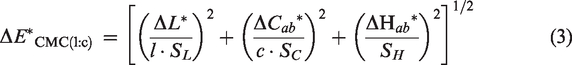
CIELAB color space is defined in Cartesian coordinates and the color difference (ΔE*) between two colors (reference and sample colors) are calculated by the CIELAB (1976) formula considering linear (Euclidean) distance between the point locations of the two colors in the space. In the calculation, the color coordinates of the two colors are taken into account and the numerical difference between the corresponding coordinates of the colors are considered. The numerical differences are presented as ΔL*, Δa*, and Δb* (where Δ = numerical value of the sample – numerical value of the reference, i.e., ΔL* = L*_sample – L*_reference). The color difference (ΔE*) according to CIELAB1976 formula is¹

{Δ E}_{a b}^{*} = \sqrt{{(Δ L^{*})}^{2} + {(Δ a^{*})}^{2} + {(Δ b^{*})}^{2}}

(1)

However, the second proposed formula CIELCh considers the coordinate differences in CIELAB color space in a different way depending on L*, C*, and h. This consideration results in the fact that CIELCh color difference equation considers the CIELAB color space in polar coordinates and computes ΔE* according to polar coordinate differences of L*, C_ab*, and h, i.e., ΔL*, ΔC*, and ΔH*:¹

{Δ E}_{a b}^{*} = \sqrt{{(Δ L^{*})}^{2} + {(Δ C^{*})}^{2} + {(Δ H^{*})}^{2}}

(2)

It is generally accepted that computing ΔE* according to polar coordinates decreases the non-uniformity effect of CIELAB color space on the results and better matches are obtained between computation and visual assessments.

The human visual system is sensitive to natural and high-chroma colors depending on their hue, chroma, and lightness. But the sensitivity is found in different characteristics in different parts of the CIELAB color space and on the a*–b* color plane. For this reason, determination of the exact combination and point of hue angle in addition to its related chroma of a color on the a*–b* color plane is important in the calculation of ΔE*. When the ΔE* observation mechanism of the human eye is taken into consideration, the human eye sees the differences in hue of the two colors at first. Chroma difference is the second property of the colors to be observed and lightness difference is recognized as the last. For this reason, the difference queue of hue (ΔH*), chroma (ΔC*), and lightness (ΔL*) becomes the most important consideration in the calculation of ΔE* between two colors (reference and sample). The intended color difference formulas should consider the differences in hue first, in chroma second, and in lightness third, to be consistent with the visual consideration of the human eye and brain. The advanced color difference formulas differ from each other in the method and how precise the calculation of hue and chroma are in the CIELAB color space.²

The concept of color is very important in human life because humans have their own individual color choices in every phase of daily life. In textiles, uniform color is important in garments because they are made of many different parts which are cut in preparation and later associated (sewn) to each other in the garment production stage. However, each part cannot be chosen from the same area (part) of the plain dyed fabric but collected from different parts of the whole fabric depending on the garment making operations which are carried out by the ready cloth making industry.² If there is a color difference between the different parts of a garment which was produced to have the same color in the whole, this color difference is considered as a failure and lack of quality of the garment. For this reason, there is a need for a precise color difference formula or color matching procedure which is consistent with the color perception properties of the human eye. Questions arise which formula should be used according to different ΔE* magnitudes in industrial applications or whether it would be possible to use a hybrid system to deal with different color difference changes.^2,3

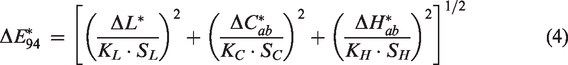
Much research has been performed on the non-uniformity property of the CIELAB color space and its possible solution via different color difference formulas. Further color difference equations CMC_(l:c),⁴ CIE94,⁵ and CIEDE2000⁶ were formulated and presented for use and research. These color difference formulas consider the same color space coordinates (L*, a*, b*, C*, and h in CIELAB color space) for ΔE* calculation but they make the computations using different color difference equations from each other. These ΔE* equations are as follows.^4
–6

i. Color difference according to the CMC_(I:c) formula:

{Δ E}^{*}_{CMC (l : c)} = {[{(\frac{Δ L^{*}}{l \cdot S_{L}})}^{2} + {(\frac{Δ {C_{a b}}^{*}}{c \cdot S_{C}})}^{2} + {(\frac{{Δ H_{a b}}^{*}}{S_{H}})}^{2}]}^{1 / 2}

(3)

where l and c are constants related to acceptance ellipsoid (user adjustable) (usually l = 2 and c = 1) and S_L, S_C, S_H are the CMC tolerance ellipsoid semi-axis lengths (weighting factors).

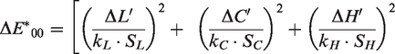
ii. Color difference according to the CIE94 formula:

{Δ E}_{94}^{*} = {[{(\frac{Δ L^{*}}{K_{L} \cdot S_{L}})}^{2} + {(\frac{Δ C_{a b}^{*}}{K_{C} \cdot S_{C}})}^{2} + {(\frac{Δ^{H_{a b}^{*}}}{K_{H} \cdot S_{H}})}^{2}]}^{1 / 2}

(4)

where S_L, S_C, S_H are CIE94 tolerance ellipsoid semi-axis lengths (weighting factors) and K_L, K_C, K_H are parametric factors (usually K_L = 2, K_C = 1, and K_H = 1).

iii. Color difference according to the CIEDE2000 formula:

{Δ E}^{*}_{00} = [{(\frac{Δ L^{'}}{k_{L} \cdot S_{L}})}^{2} + {(\frac{Δ C^{'}}{k_{C} \cdot S_{C}})}^{2} + {(\frac{Δ H^{'}}{k_{H} \cdot S_{H}})}^{2}

{+ R_{T} (\frac{Δ C^{'}}{k_{C} \cdot S_{C}}) {(\frac{Δ H^{'}}{k_{H} \cdot S_{H}})]}^{}}^{1 / 2}

(5)

where L′, C′, and H′ are derived values from L*, C*, and H according to the CIEDE2000 formula, S_L, S_C, S_H are CIDE2000 tolerance ellipsoid semi-axis lengths (weighting factors), K_L, K_C, K_H are parametric factors (usually K_L = 2, K_C = 1, and K_H = 1), and R_T is the hue rotation term.

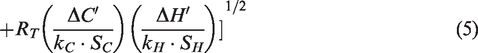
These three ΔE* formulas consider the CIELAB color space and in addition calculate ΔE* in polar coordinates, not Cartesian coordinates. They all try to describe the color primarily by the correct hue angle (h), hue difference (ΔH*), choma (C_ab*), and chroma difference (ΔC*). Because of the non-uniformity of the CIELAB color space, these three formulas compute an acceptability ellipsoid around the reference color point (a* and b* coordinates of the reference color) in the CIELAB color space which the ellipsoid volume tries to match with the visual perception of the human eye. By the formation of a color acceptance ellipsoid by taking the reference color in the center of the volume, the three color difference formulas give better color matching results with the human eye. The CIEDE2000 formula, being different from the color coordinate dependence in the color space, calculates further color coordinates as L’, a’, b’, and C’ by using CIELAB coordinates and tries to perform a better positioning of the reference color in the color space.^7
–12

In addition to the research into new and more reliable color difference formulas, the researchers tried to express and place the colors in a more uniform color space. Instead of replacing formulating colors in a color space, studies focused on alternative color placement, and color appearance models (CAMs) were proposed and discussed.^13
–15 Visual experiments resulted in that the further defined CIECAM02 space was also not perceptually uniform and new color formulas could be applied to enhance the correlation to the visual data.¹⁴

The CIEDE2000 color difference formula was adopted to allow a better calculation of small color differences and the equation related to the computation of CIEDE2000 consider the different parts of the CIELAB color space in different ways. Considering that different color difference formulas could be taken into consideration, CIE recommended the CAM CIECAM02. It was considered to form three new color spaces as CAM02-SDC, CAM02-LCD, and CAM02-UCS, for estimating small, large, and overall ranges of color differences, respectively.^2,16

The researchers focused on the problem that the current color spaces cannot give consistent color difference results in accordance with the observations made by the human eye. For this reason, alternative color difference formulas were proposed which try to correlate their computation with the perception property of the human eye by defining an acceptance ellipsoid volume around the reference color. The performances of CIELAB-based color difference formulas were tested for small and large color differences.^2,16
–20

The research described here was focused on the color difference results of the four color difference formulas on the a*–b* color plane by changing a* and b* coordinates in a regular way at a constant lightness value of L* = 50. Color difference computing properties of CIELAB1976, CMC, CIE94, and CIDE2000 were tested at a constant lightness value on the a*–b* color plane. The ΔE* results showed distinct differences depending on the Cartesian or polar considerations of the different formulas. The CMC formula used a very different method of computation in certain hue regions and chroma changes from the other three formulas, especially at increasing a* coordinate differences. The possibility to use different color difference formulas in different hue regions of the a*–b* color plane was discussed in the search for consistent color difference decisions.

Materials and method

The aim of the current research was to investigate whether there is a possibility of using different color difference equations in different hue regions of the a*–b* color plane in the CIELAB color space for a better interpretation of the ΔE* results and to understand the computing differences of the four color difference formulas for regular coordinate changes. The dependence of the four most important and widely used color difference formulas (CIELAB1976, CMC (2:1), CIE94 (2:1:1), and CIEDE2000 (2:1:1)) were tested by regular coordinate changes on the a*–b* color plane and their computing differences in different hue regions (quarters) at constant lightness (L* = 50) were obtained. The purpose of computing was to investigate the ΔE* calculation differences and properties of the four formulas in the four different hue regions (hue quarters) of the a*–b* color plane of the CIELAB color space (at a constant lightness value of L* = 50).

In order to make the computing, a special software was prepared by using C# programming. Color difference formulas were prepared as Excel worksheets in the software (program) and used as the computation references. The prepared C# software computed ΔE* results of the four color difference formulas, again in Excel worksheets, between the chosen coordinate ranges. The start and end coordinates (points; or a* and b* coordinates) together with constant coordinate (L* = 50) were adjusted in the computations.

The CIELAB1976 equation calculates ΔE* via Cartesian coordinates and considers the differences between reference and sample colors over their locations in CIELAB color space by computing ΔL*, Δa*, and Δb*. However, the other three color difference formulas calculate ΔE* via polar coordinates and consider the differences between reference and sample colors by computing ΔL*, ΔC*, and ΔH*. The three formulas CMC, CIE94, and CIEDE2000 first consider hue (h) and chroma (C*) and their differences (ΔH* and ΔC*) on the a*–b* color plane. All four formulas use the same CIELAB color space coordinates (L*, a*, b*, C_ab*, and h) for the calculation of ΔE* between reference and sample colors in the CIELAB color space. But they each calculate ΔE* with different mathematical equations considering different priorities in the color space. The main priorities that they consider are hue angle and chroma differences. For that reason, the four color difference formulas have the property of finding different “ΔE*” color difference values by using the same fixed (reference and sample) color coordinates. The ΔE* values calculated by the four color difference formulas could show distinct differences from each other depending on the chromaticity properties (h and C* in color space) of the reference and sample colors on the a*–b* color plane. The purpose of this paper is to investigate the color difference calculation properties of the four color difference formulas under fixed coordinate changes in the CIELAB color space.

The CIELAB color space is not a perceptually uniform space, which means that equal ΔE* values calculated by a color difference formula do not correspond to equal visual differences observed by the human eye (human observer). All four color difference formulas define an acceptability volume (tolerance volume) around the coordinates of the reference color in CIELAB color space. The acceptability volume changes from a cube (CIELAB1976) to an acceptance ellipsoid (CMC, CIE9, and CIEDE2000) as a result of the consideration of the color coordinates according to Cartesian or polar coordinates (coordinate differences calculation). This research investigated the results of color difference calculations of the four color difference (tolerance) formulas by using a specially prepared computer software. The validity of the computed results was also checked by a commercially used software and by a well-known and reliable internet site calculator.²¹ The results are presented in the corresponding figures.

In order to simplify the figures, every fifth calculated color difference result was presented and the four results between them were omitted from the figures. In addition, the obtained ΔE* were attained by first-order or (near-)second-order polynomial equations in order to make a better presentation. Some equations contain upper case Euler’s number coefficients which Excel computed in order to consider all the figure points in equations. For that reason, although some equations may have a second-order coefficients with very small Euler’ numbers, they could be taken as first-order equations.

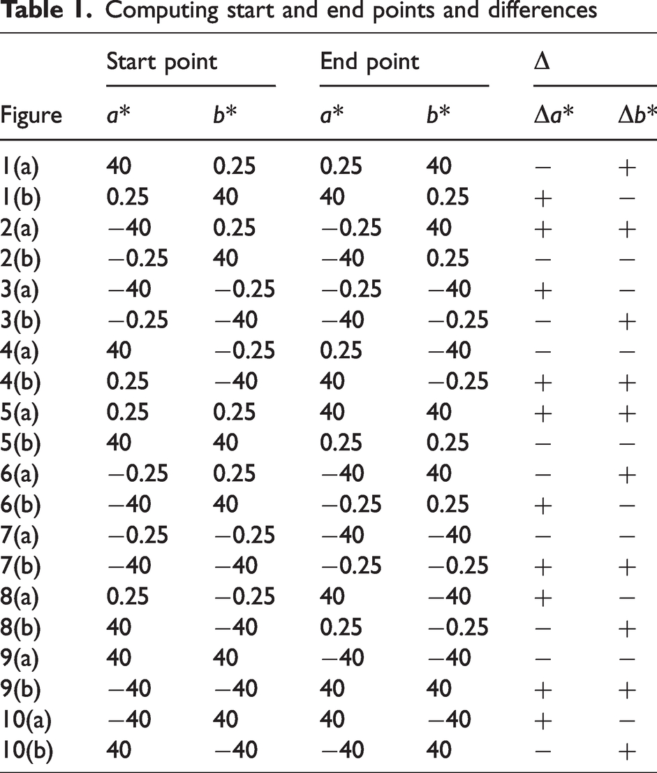
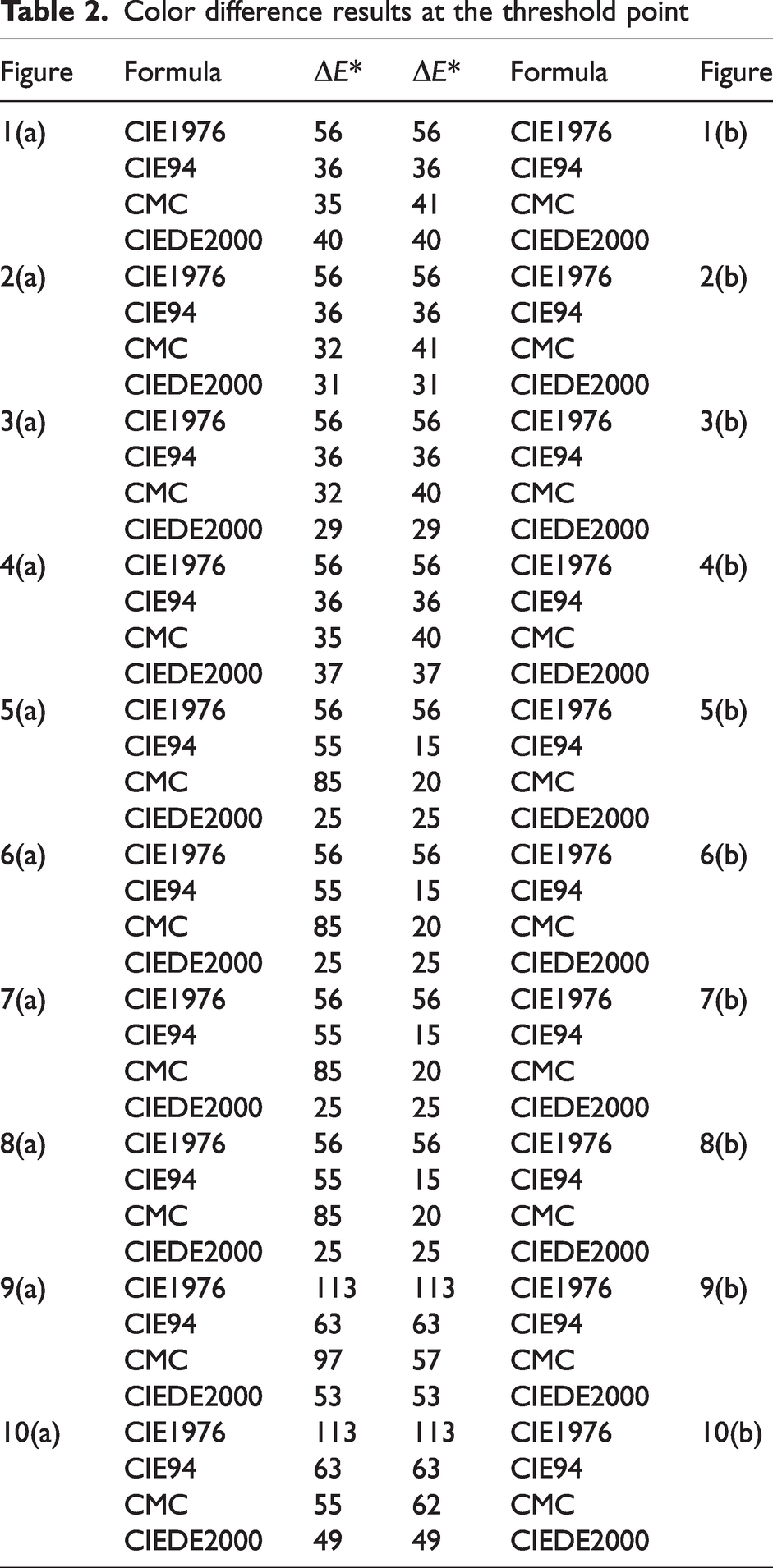
The start and end points considered in the figures in addition to the sign of Δ are presented in Table 1. The ΔE* results obtained at the threshold coordinate points (taking the start point as a reference and the end point as the sample color) are presented in Table 2.

Table 1.

Computing start and end points and differences

Figure	Start point		End point		Δ
Figure	a*	b*	a*	b*	Δa*	Δb*
1(a)	40	0.25	0.25	40	−	+
1(b)	0.25	40	40	0.25	+	−
2(a)	−40	0.25	−0.25	40	+	+
2(b)	−0.25	40	−40	0.25	−	−
3(a)	−40	−0.25	−0.25	−40	+	−
3(b)	−0.25	−40	−40	−0.25	−	+
4(a)	40	−0.25	0.25	−40	−	−
4(b)	0.25	−40	40	−0.25	+	+
5(a)	0.25	0.25	40	40	+	+
5(b)	40	40	0.25	0.25	−	−
6(a)	−0.25	0.25	−40	40	−	+
6(b)	−40	40	−0.25	0.25	+	−
7(a)	−0.25	−0.25	−40	−40	−	−
7(b)	−40	−40	−0.25	−0.25	+	+
8(a)	0.25	−0.25	40	−40	+	−
8(b)	40	−40	0.25	−0.25	−	+
9(a)	40	40	−40	−40	−	−
9(b)	−40	−40	40	40	+	+
10(a)	−40	40	40	−40	+	−
10(b)	40	−40	−40	40	−	+

Table 2.

Color difference results at the threshold point

Figure	Formula	ΔE*	ΔE*	Formula	Figure
1(a)	CIE1976	56	56	CIE1976	1(b)
	CIE94	36	36	CIE94
	CMC	35	41	CMC
	CIEDE2000	40	40	CIEDE2000
2(a)	CIE1976	56	56	CIE1976	2(b)
	CIE94	36	36	CIE94
	CMC	32	41	CMC
	CIEDE2000	31	31	CIEDE2000
3(a)	CIE1976	56	56	CIE1976	3(b)
	CIE94	36	36	CIE94
	CMC	32	40	CMC
	CIEDE2000	29	29	CIEDE2000
4(a)	CIE1976	56	56	CIE1976	4(b)
	CIE94	36	36	CIE94
	CMC	35	40	CMC
	CIEDE2000	37	37	CIEDE2000
5(a)	CIE1976	56	56	CIE1976	5(b)
	CIE94	55	15	CIE94
	CMC	85	20	CMC
	CIEDE2000	25	25	CIEDE2000
6(a)	CIE1976	56	56	CIE1976	6(b)
	CIE94	55	15	CIE94
	CMC	85	20	CMC
	CIEDE2000	25	25	CIEDE2000
7(a)	CIE1976	56	56	CIE1976	7(b)
	CIE94	55	15	CIE94
	CMC	85	20	CMC
	CIEDE2000	25	25	CIEDE2000
8(a)	CIE1976	56	56	CIE1976	8(b)
	CIE94	55	15	CIE94
	CMC	85	20	CMC
	CIEDE2000	25	25	CIEDE2000
9(a)	CIE1976	113	113	CIE1976	9(b)
	CIE94	63	63	CIE94
	CMC	97	57	CMC
	CIEDE2000	53	53	CIEDE2000
10(a)	CIE1976	113	113	CIE1976	10(b)
	CIE94	63	63	CIE94
	CMC	55	62	CMC
	CIEDE2000	49	49	CIEDE2000

Results and discussion

Dependences of the four color difference formulas on the regular changes in red–green axis (a*) and yellow–blue axis (b*) coordinates at constant lightness value of L* = 50 were presented in the following figures for different start and end points. All the ΔE* computations were performed on the a*–b* color plane at L* = 50. In all figures (Figures 1 –10), a* and b* coordinates were increased or decreased between ±40 numerical values by 0.25 unit regular steps in the four hue regions of the a*–b* color plane.

Figure 1.

Color difference results: (a) from a* = 40, b* = 0.25 to a* = 0.25, b* = 40; L* = 50; (b) from a* = 0.25, b* = 40 to a* = 40, b* = 0.25; L* = 50.

Figure 2.

Color difference results: (a) from a* = −40, b* = 0.25 to a* = −0.25, b* = 40; L* = 50; (b) from a* = −0.25, b* = 40 to a* = −40, b* = 0.25; L* = 50.

Figure 3.

Color difference results: (a) from a* = −40, b* = −0.25 to a* = −0.25, b* = −40; L* = 50; (b) from a* = −0.25, b* = −40 to a* = −40, b* = −0.25; L* = 50.

Figure 4.

Color difference results: (a) from a* = 40, b* = −0.25 to a* = 0.25, b* = −40; L* = 50; (b) from a* = 0.25, b* = −40 to a* = 40, b* = −0.25; L* = 50.

Figure 5.

Color difference results: (a) from a* = 0.25, b* = 0.25 to a* = 40, b* = 40; L* = 50; (b) from a* = 40, b* = 40 to a* = 0.25, b* = 0.25; L* = 50.

Figure 6.

Color difference results: (a) from a* = −0.25, b* = 0.25 to a* = −40, b* = 40; L* = 50; (b) from a* = −40, b* = 40 to a* = −0.25, b* = 0.25; L* = 50.

Figure 7.

Color difference results: (a) from a* = −0.25, b* = −0.25 to a* = −40, b* = −40; L* = 50; (b) from a* = −40, b* = −40 to a* = −0.25, b* = −0.25; L* = 50.

Figure 8.

Color difference results: (a) from a* = 0.25, b* = −0.25 to a* = 40, b* = −40; L* = 50; (b) from a* = 40, b* = −40 to a* = 0.25, b* = −0.25; L* = 50.

Figure 9.

Color difference results: (a) from a* = 40, b* = 40 to a* = −40, b* = −40; L* = 50; (b) from a* = −40, b* = −40 to a* = 40, b* = 40; L* = 50.

Figure 10.

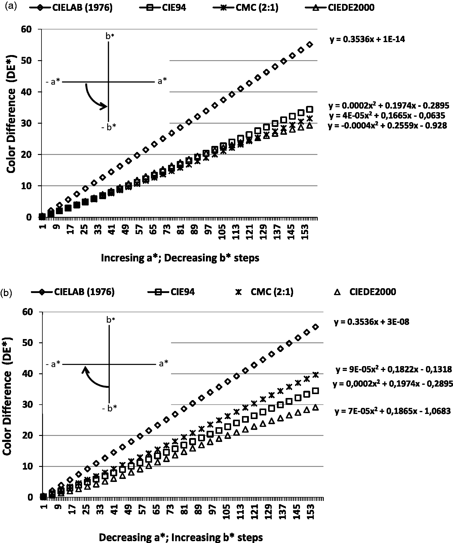
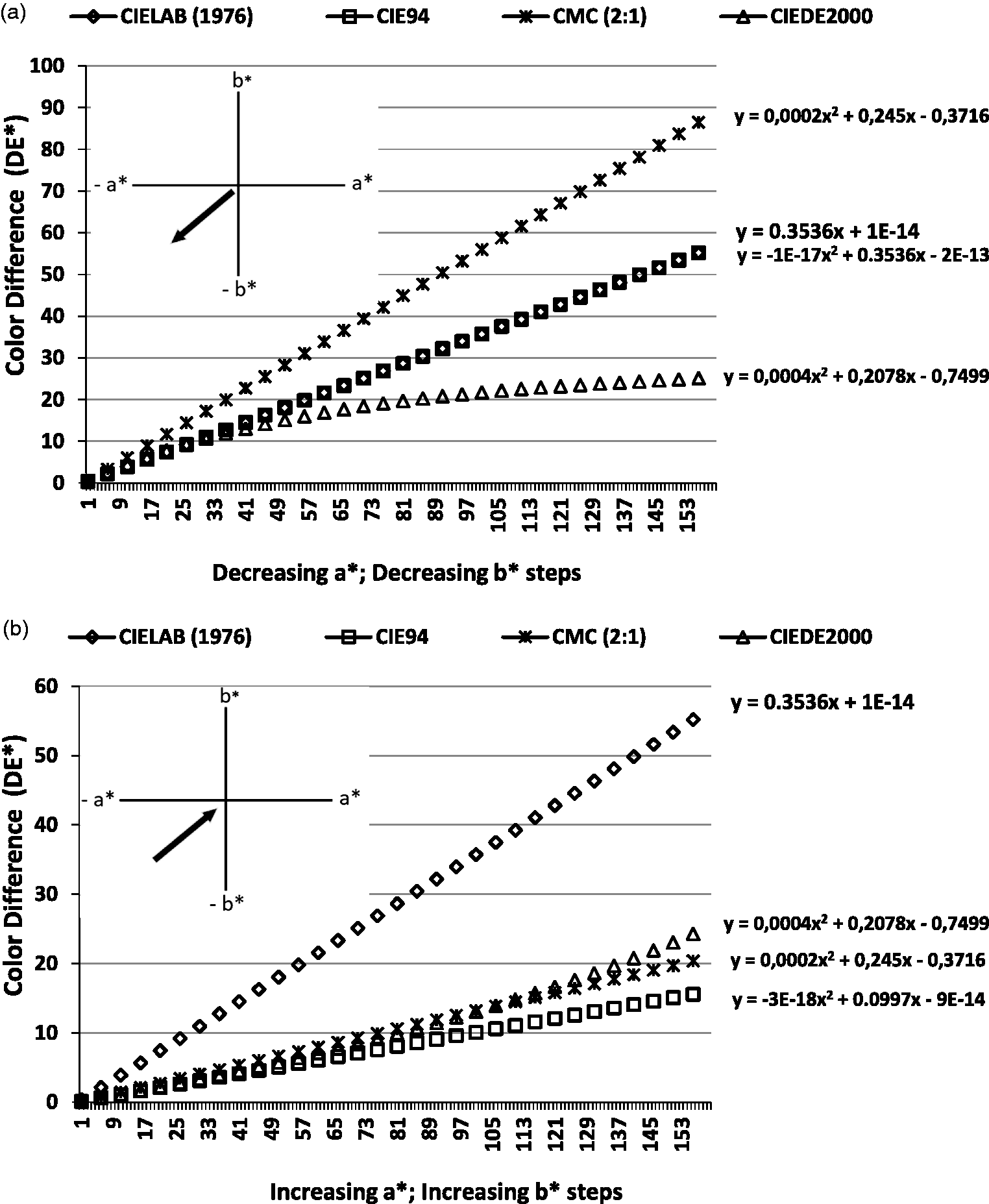
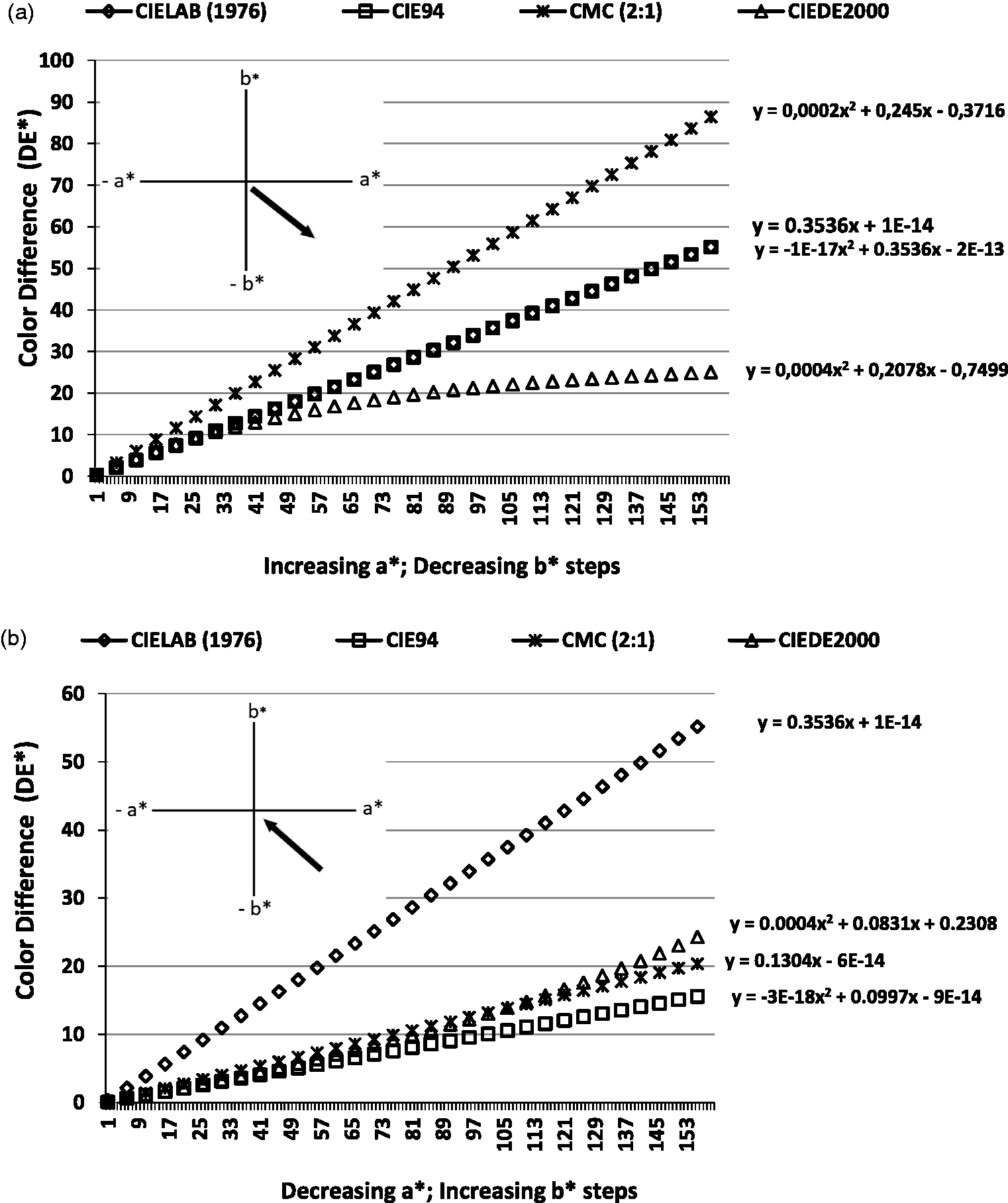
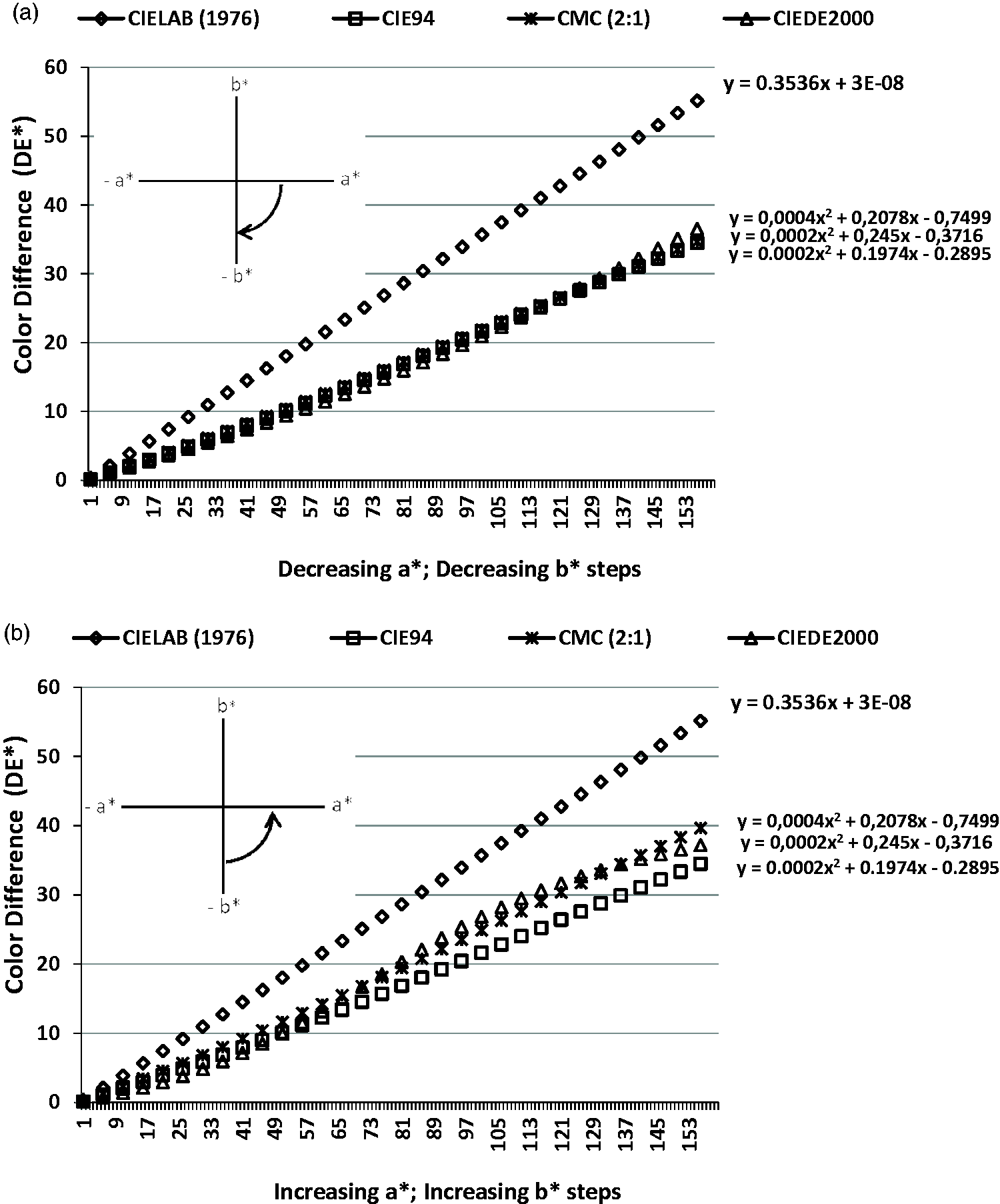
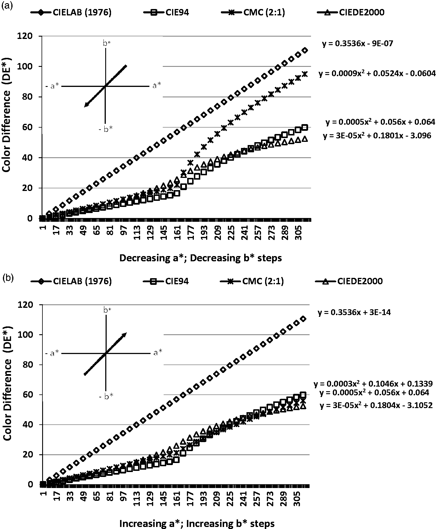
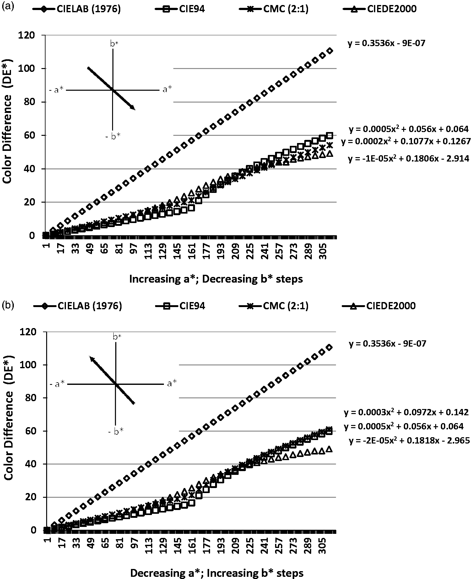
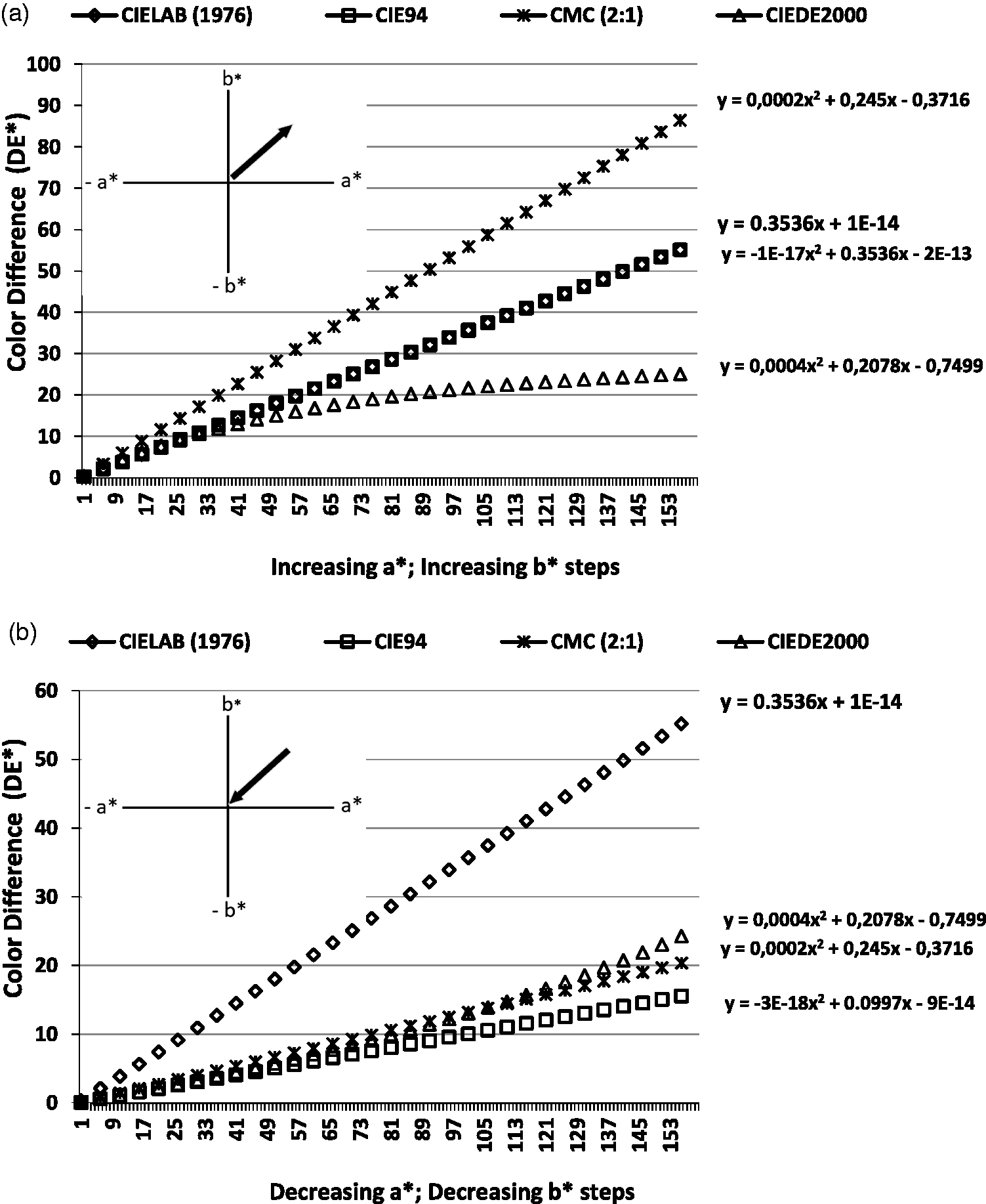
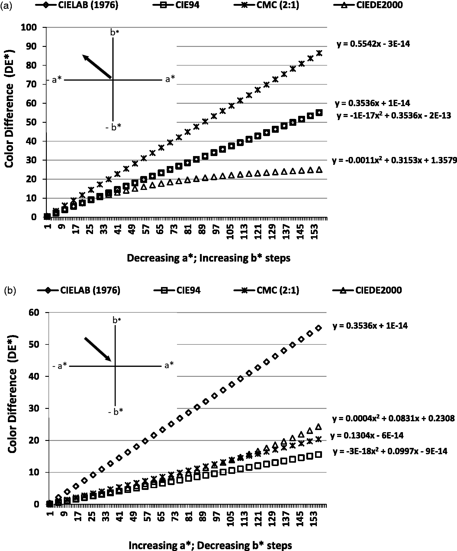
Color difference results: (a) from a* = −40, b* = 40 to a* = 40, b* = −40; L* = 50; (b) from a* = 40, b* = −40 to a* = −40, b* = 40; L* = 50.

The CIELAB1976 equation calculates ΔE* in Cartesian coordinates. Because of that reason the same corresponding ΔE* values in addition to a straight line of the first order were obtained in the calculations which are presented in Figures 1 –4, Figures 5 –8, and Figures 9 and 10. The start and end points differed in the corresponding Figures 1 –8 and Figures 9 and 10. Although the CIE94 equation calculates ΔE* in polar coordinates, a very similar but not identical calculation behavior to CIELAB1976 was obtained for CIE94 in Figures 1 –4 and in Figures 5 –8. The computed ΔE* results of CIE94 were almost linear although it considers polar coordinates.

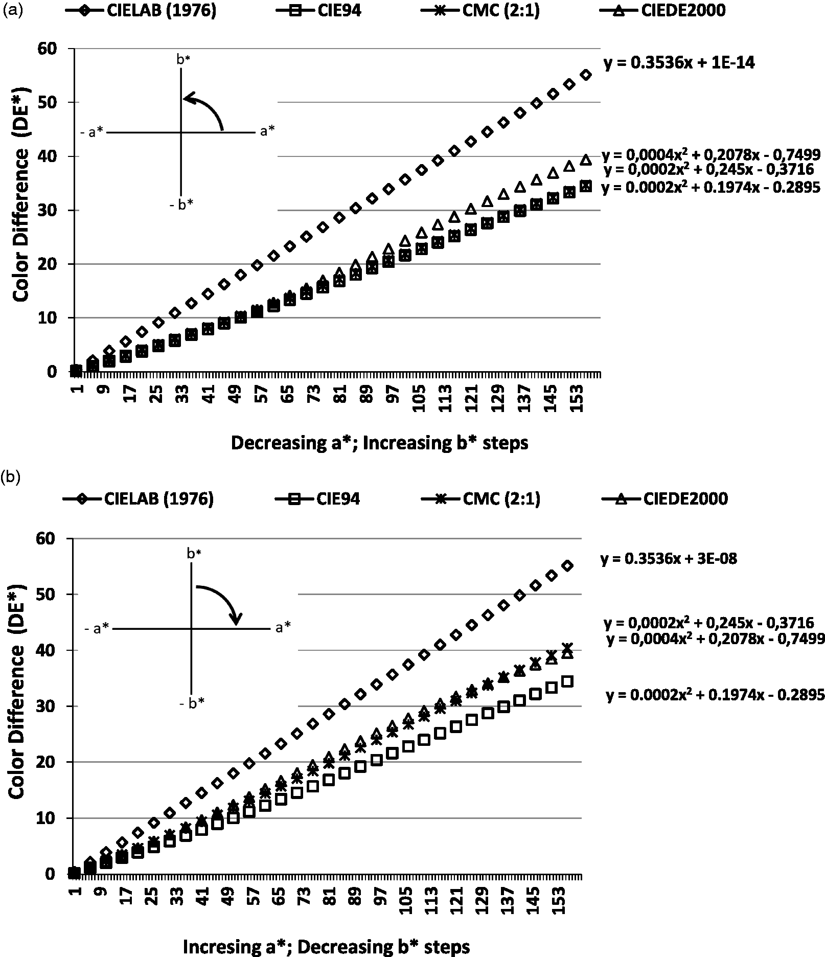
In Figures 1 –4, the results for the computing directions where a* coordinates approached ±0.25 (approached the gray point) are presented in part (a) and the results in the computing directions where a* coordinates departed from ±0.25 (departed from the gray point) are presented in part (b). The computing directions are also drawn on the left-hand sides of the figures.

The a* and b* coordinates were changed correspondingly between numerical values of 40 and 0.25 by regularly increasing or decreasing the first hue region (hue quarter 0–90°) of the a*–b* color plane by units of 0.25 in Figure 1(a) and (b).

Figure 1(a) presents the computed ΔE* results of the four color difference formulas in the first hue region of the a*–b* color plane where a* coordinates decreased from 40 to 0.25 and b* coordinates increased from 0.25 to 40 by regular steps of 0.25 units. The starting point at a* = 40 and b* = 0.25 (L* = 50) was taken as the reference color and the coordinates obtained by 0.25 step changes were taken as sample colors until the point a* = 0.25 and b* = 40 was reached. Both the hue and chroma coordinates of the sample colors changed regularly depending on the start and end points.

CIELAB1976 formula computed the highest ΔE* values whereas CMC and CIE94 formulas computed the lowest ΔE* values under the selected coordinate changes. The three formulas other than CIELAB1976 presented almost similar calculation behavior in the computing through the coordinate start and end thresholds. In contrast to the changing steps presented in Figure 1(a), the a* coordinates increased from 0.25 to 40 and b* coordinates decreased from 40 to 0.25 in Figure 1(b). The starting point at a* = 0.25 and b* = 40 (L* = 50) was taken as the reference color and the coordinates obtained by 0.25 step changes were taken as sample colors until the point a* = 40 and b* = 0.25 was reached. Both the hue and chroma coordinates of the sample colors changed regularly depending on the start and end points. The highest ΔE* were obtained by computing according to CIELAB1976 which were the same as presented in Figure 1(a). The lowest ΔE* were obtained by computing according to CIE94 which the latter result is similar to the corresponding results presented in Figure 1(a). In addition, almost the same corresponding ΔE* values were obtained by computing according to CIE94 and CIEDE2000 in parts (a) and (b) of Figure 1. The CMC formula computed different ΔE* results in Figure 1(a) and (b). The same fitting polynomial equations were obtained in Figure 1(a) and (b). However, it must be stated that obtaining the same fitting polynomial equation (CMC values in Figure 1(a) and (b)) does not mean the same ΔE* results were obtained.

A brief discussion about Figure 1 implies that the CIELAB1976, CIE94, and CIEDE2000 formulas gave almost identical results in the first hue region for increasing and decreasing a* and b* coordinates (Figure 1(a) and (b)). However, ΔE* computed according to CMC presented distinctly different results depending on the direction of ΔE* computation. It must also be stated that both hue and chroma values changed in the computations presented in Figure 1. This peculiar computing behavior of the CMC formula was observed when the numerical values of a* and b* coordinates changed between 40 and 0.25. Computing behaviors of CIELAB1976, CIE94, and CIEDE2000 remained unchanged whereas CMC showed major computing changes between Figure 1(a) and Figure 1(b).

The a* and b* coordinates were changed correspondingly between numerical values of ±40 and 0.25 by increasing or decreasing by regular 0.25 units in the second hue region (hue quarter 90–180°) of the a*–b* color plane in Figure 2(a) and (b).

Figure 2(a) presents the computed ΔE* results of the four color difference formulas in the second hue region of the a*–b* color plane where a* coordinates increased from −40 to −0.25 and b* coordinates increased from 0.25 to 40 by regular steps of 0.25 units. The starting point at a* = −40 and b* = 0.25 (L* = 50) was taken as the reference color and the coordinates obtained by 0.25 step changes were taken as sample colors until the point a* = −0.25 and b* = 40 was reached. Both the hue and chroma coordinates of the sample colors changed regularly depending on the start and end points.

The CIELAB1976 formula computed the highest and CIEDE2000 and CMC formulas computed the lowest ΔE* values under the selected coordinate changes. CIEDE2000 and CMC computed lower ΔE* values than CIE94 and than their corresponding values given in Figure 1(a). In contrast to the step changes presented in Figure 2(a), a* coordinates decreased from −0.25 to −40 and b* coordinates decreased from 40 to 0.25 by regular steps of 0.25 units in Figure 2(b). The starting point at a* = −0.25 and b* = 40 (L* = 50) was taken as the reference color and the coordinates obtained by 0.25 step changes were taken as sample colors until the point a* = −40 and b* = 0.25 was reached. Both the hue and chroma coordinates of the sample colors changed regularly depending on the start and end points. Similar to the results presented in Figure 2(a), the highest ΔE* values were obtained by computing according to CIELAB1976. The lowest ΔE* values were obtained by computing according to CIEDE2000. In addition, CIE94 computed the same ΔE* values in Figure 2(a) and (b), similar to those presented in Figure 1. However, the same corresponding ΔE* values were obtained by computing according to CMC in Figures 1(b) and 2(b) but different ΔE* values were obtained in Figures 1(a) and 2(a).

A brief discussion of Figure 2 implies that CIELAB1976, CIE94, and CIEDE2000 formulas gave almost identical results in the second hue region for increasing and decreasing a* and b* coordinates, similar to the results obtained in Figure 1. However, CMC computed distinctly different results depending on the direction of computation of ΔE*, similar to Figure 1. This peculiar computing behavior of the CMC formula was observed when the a* coordinates changed between 0.25 and 40. This behavior was very similar to the results obtained in Figure 1(b). According to the results presented in Figure 1(b) and Figure 2(b), it could be stated that the CMC formula computes the color difference results in its own peculiar way when a* coordinates changed their numeric value from ±0.25 to ±40 and b* coordinates change their numeric values between 40 to 0.25 at the same time. The CMC formula computed different ΔE* results when a* coordinates approached the gray point (part (a)) but it computed the same ΔE* results when a* coordinates departed from the gray point (part (b)) in Figures 1 and 2.

Correspondingly the same polynomial behaviors of the four formulas could be observed as the computed color difference values increased in Figures 1 and 2.

The a* and b* coordinates were changed correspondingly between numerical values of −40 and −0.25 by regular increases or decreases of 0.25 units in the third hue region (hue quarter 180–270°) of the a*–b* color plane in Figure 3(a) and (b).

Figure 3(a) presents the computed ΔE* results of the four color difference formulas in the third hue region of the a*–b* color plane where a* coordinates decreased from −40 to −0.25 and b* coordinates increased from −0.25 to −40 by regular steps of 0.25 units. The starting point at a* = −40 and b* = −0.25 (L* = 50) was taken as the reference color and the coordinates obtained by 0.25 step changes were taken as sample colors until the point a* = −0.25 and b* = −40 was reached. Both the hue and chroma coordinates of the sample colors changed regularly depending on the start and end points.

CIELAB1976 formula computed the highest while CIEDE2000 formula computed the lowest ΔE* values under the selected coordinate changes. These findings were very similar to the corresponding ones presented in Figure 2(a). In addition, the computed ΔE* results of CMC were the same as the corresponding results presented in Figure 2(a). Opposite to the changing steps presented in Figure 3(a), a* coordinates decreased from −0.25 to −40 and b* coordinates increased from −40 to −0.25 by regular steps of 0.25 units in Figure 3(b). The starting point at a* = −0.25 and b* = −40 (L* = 50) was taken as the reference color and the coordinates obtained by 0.25 step changes were taken as sample colors until the point a* = −40 and b* = −0.25 was reached. Both the hue and chroma coordinates of the sample colors changed regularly depending on the start and end points. The highest ΔE* values were obtained by computing according to CIELAB1976 and the lowest ΔE* values were obtained by computing according to CIEDE2000, similar to Figure 3(a). Almost the same corresponding ΔE* values were obtained for CIE94 and CIEDE2000 in Figures 3(a) and (b). In Figure 3(b), much higher ΔE* values were obtained according to the computation by CMC than the corresponding values in Figure 3(a). In addition, different polynomial equations were obtained for CIEDE2000 and CMC.

A brief discussion of Figure 3 implies that the CIELAB1976, CIE94, and CIEDE2000 formulas computed almost identical results in the third hue region for increasing and decreasing a* and b* coordinates, similar to the results obtained in Figures 1 and 2. However, the CMC formula computed different ΔE* results in Figure 3(a) and (b) in which the computing behavior was the same as in the corresponding results presented in Figures 1(b) and 2(b). In the third region of the a*–b* color plane where a* and b* coordinates always take negative signs and numerical values, the ΔE* computing according to CIEDE2000 formula gave the lowest ΔE* results whether a* and b* coordinates increased or decreased. The ΔE* results presented in Figures 1(b), 2(b), and 3(b) implied that computing according to the CMC formula calculated higher color difference results when a* coordinates numerically increased (from 0.25 to 40) and b* coordinates decreased (from 40 to 0.25).

The a* and b* coordinates were changed correspondingly between numerical values of ±40 and ±0.25 by regularly increasing or decreasing by 0.25 units in the fourth hue region (hue quarter 270–360° (0°)) of the a*–b* color plane in Figure 4(a) and (b).

Figure 4(a) presented the computed ΔE* results of the four color difference formulas in the fourth hue region of the a*–b* color plane where a* coordinates decreased from 40 to 0.25 and b* coordinates decreased from −0.25 to −40 by regular steps of 0.25 units. The starting point at a* = 40 and b* = −0.25 (L* = 50) was taken as the reference color and the coordinates obtained by 0.25 step changes were taken as sample colors until the point a* = 0.25 and b* = −40 was reached. Both the hue and chroma coordinates of the sample colors changed regularly depending on the start and end points.

The highest ΔE* values were obtained by computing according to the CIELAB1976 formula and the lowest ΔE* values were obtained by computing according to the CMC, CIE94, and CIEDE2000 formulas. These three formulas gave almost the same ΔE* results in the corresponding thresholds. The CIEDE2000 formula computed the highest ΔE* values after CIELAB1976. These findings were similar to the corresponding ones presented in Figure 1(a).

Opposite to the changing steps presented in Figure 4(a), a* coordinates increased from 0.25 to 40 and b* coordinates increased from −40 to −0.25 by regular steps of 0.25 units in Figure 4(b). The starting point at a* = 0.25 and b* = −40 (L* = 50) was taken as the reference color and the coordinates obtained by 0.25 step changes were taken as sample colors until a* = 40 and b* = −0.25 point was reached. Both the hue and chroma coordinates of the sample colors changed regularly depending on the start and end points. The highest ΔE* were obtained by computing according to CIELAB1976 and the lowest ΔE* values were obtained by computing according to CIE94 and CIEDE2000, similar to the results presented in Figure 1(b). CMC computed the next highest ΔE* results after CIELAB1976.

A brief discussion of Figure 4 implies that the CIELAB1976, CIE94, and CIEDE2000 formulas computed almost identical results in the fourth region of the a*–b* color plane for increasing and decreasing a* and b* coordinates. However, similar to Figures 1 –3, the CMC formula computed distinctly different ΔE* values in Figure 4(a) and (b). The same polynomial second-order equation was obtained for CMC color difference plots in Figure 4(a) and (b) but the resultant numerical ΔE* values were completely different. CMC computed different ΔE* values when a* and b* coordinates were increased and decreased but the computed color differences followed a special numerical order that although the resultant ΔE* values were different, their changing property was the same.

The computed ΔE* values taking the start points as the reference color and only the end points as the sample color are presented in Table 2. The computed threshold ΔE* values of Figures 1 –4 showed similarities and dissimilarities in Table 2. It could be readily observed that CIELAB1976 and CIE94 formulas always computed the same ΔE* results (CIELAB1976 ΔE* = 56 and CIE94 ΔE* = 36) whether a* and b* coordinates increased or decreased in the four hue regions of the a*–b* color plane. CMC formula computed the same ΔE* values in Figures 1(a) and 4(a) when a* coordinates approached the gray point and b* coordinates departed from the gray point (CMC ΔE* = 35). In both computations, a* coordinates always took the positive values (hue region I and hue region IV). In addition, the same computing behavior of CMC formula was observed in Figures 2(a) and 3(a) (CMC ΔE* = 32) when negative a* coordinates approached the gray point (hue regions II and III) and b* coordinates departed from the gray point (from 0.25 to 40). Similar to those observations, the ΔE* values computed according to CMC formula were the same (CMC ΔE* = 41) in Figures 1(b) and 2(b) where a* coordinates positively or negatively departed from the gray point (±0.25 to ±40) and positive b* coordinates approached the gray point (40 to 0.25). The CMC formula computed the same ΔE* values in Figures 3(b) and 4(b) where positive or negative a* coordinates departed from the gray point (±0.25 to 40) and negative b* coordinates approached the gray point (–40 to −0.25).

Similar to the computing behavior of CMC, the CIEDE2000 formula computed similar and dissimilar ΔE* results in Figures 1 –4. The threshold computed results presented in Table 2 revealed that CIEDE2000 formula resulted in the same ΔE* values when computing was performed in the same hue region whether a* and b* coordinates increased or decreased (parts (a) and (b) in Figures 1 –4), but it resulted in different ΔE* values when the hue region differed (in Figures 1 –4, hue regions I, II, III, and IV). The CIEDE2000 formula computed its highest ΔE* results in the first hue region (Figure 1(a) and (b)) and its lowest ΔE* results in the third hue region (Figure 3(a) and (b)). In Figures 1 –4 where hue and chroma values and their corresponding differences changed regularly with respect to a* and b* coordinates, CMC computing results differed from each other whether the coordinates increased or decreased in the same hue region. However, CIEDE2000 computed the same ΔE* results in the same hue region but different ΔE* results in different hue regions.

The different computing behaviors of the CMC and CIEDE2000 formulas in the hue regions were because of the acceptance ellipsoid semi-axes calculations. Both formulas calculate their corresponding hue semi-axis value (S_H) according to the hue angle changes in the color space.^4,6 However, although the CIE94 formula calculates ΔE* according to polar coordinates, it calculates the S_H semi-axis depending on C* of the reference color.⁵ In addition, CMC and CIEDE2000 compute ΔH* considering the hue angles of reference and sample colors. Although CMC, CIE94, and CIEDE2000 calculate ΔE* in polar coordinates, the reason for their different computing behaviors in different hue regions of the a*–b* color plane is the computing difference of their acceptance ellipsoid semi-axis, mainly S_H, and ΔH*. In Figures 1 –4, hue angles and their differences in computing ΔE* correspondingly changed from 0° to 360° but the differences in chroma (ΔC_ab*) were always the same. In Figures 1 –4, ΔL* values were always zero and ΔC_ab* were always the same, but ΔH* changed according to the different equations of CMC and CIEDE2000. In addition, their ellipsoid semi-axes lengths (mainly S_H) were computed depending on the position of the reference color on a*–b* color plane.

Different computing directions were tested in Figures 5 –8. The computing start and end points were selected as ±0.25 and ±40 for both a* and b* coordinates in the four hue regions. Similar to the results presented in Figures 1 –4, CIE1796 and CIE94 formulas computed almost linear and correspondingly the same of their ΔE* values in Figures 5 –8. The computing was performed on straight directions in which chroma differences were obtained but hue angles were the same (45° (first region); 135° (second region); 225° (third region); and 315° (fourth region)). As a result, any hue difference (ΔH*) was not calculated in the color difference formulas in the computing besides the lightness difference (ΔL* = 0).

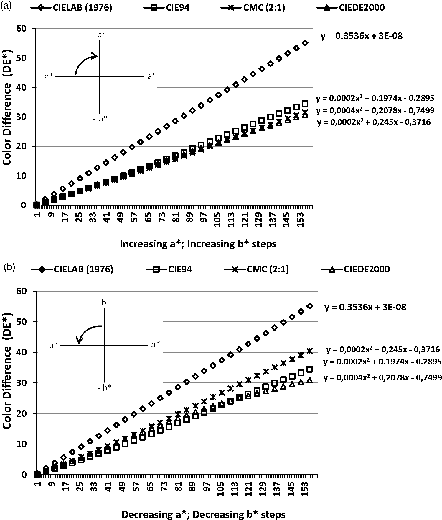
The a* and b* coordinates were changed correspondingly between numerical values of 0.25 and 40 by regularly increasing and decreasing by 0.25 units in the first hue region (hue quarter 0–90°) of the a*–b* color plane in Figure 5(a) and (b).

Figure 5(a) presents the computed color difference results of the four ΔE* formulas in the first hue region of the a*–b* color plane where both a* and b* coordinates increased from 0.25 to 40 by regular steps of 0.25 units. The starting point a* = b* = 0.25 (L* = 50) was taken as the reference color and the coordinates obtained by 0.25 step changes (increases) were taken as sample colors until the point a* = b* = 40 was reached. The highest ΔE* values were obtained by computing according to CMC and the lowest ΔE* values were obtained by computing according to CIEDE2000. The same ΔE* values were obtained by computing according to CIELAB1976 and CIE94 formulas. A descending curve was obtained for CIEDE2000 which implied that the CIEDE2000 formula became insensitive to the coordinate numerical increases in the farthest parts (high chroma values) of the first hue region and did not differentiate as the chroma difference increased. Opposite to the changing steps given in Figure 5(a), both a* and b* coordinates decreased from 40 to 0.25 by regular steps of 0.25 units in Figure 5(b). The starting point at a* = b* = 40 was taken as the reference color and the coordinates obtained by 0.25 step changes (decreases) were taken as sample colors until the point a* = b* = 0.25 was reached. The highest ΔE* values were obtained by computing according to CIELAB1976 and the lowest ΔE* values were obtained by computing according to CIE94. The computed results were very much different from those presented in Figure 5(a) although only the ΔE* computing direction was reversed. Only the CIELAB1976 formula did not change its computing character because of its Cartesian property and the same color difference values were obtained. However, the other three formulas computed distinctly different values in parts (a) and (b) of Figure 5, especially CMC and CIE94.

A brief discussion of Figure 5 implied that only the CIELAB1976 formula gave consistent ΔE* calculations whether a* and b* coordinates increased or decreased according to a chroma direction. The computation of ΔE* was basically performed on the chroma axis at 45° of the first hue region. However, the ΔE* computing behaviors of the other three formulas were very much different at increasing and decreasing coordinate directions. Lower color difference values were obtained by computing according to CIE94 and CMC but slightly higher ΔE* values were obtained by computing according to CIEDE2000 in part (b) than part (a) of Figure 5.

The a* and b* coordinates were changed correspondingly between numerical values of ±0.25 and ±40 by regularly increasing and decreasing by 0.25 units in the second hue region (hue quarter 90–180°) of the a*–b* color plane in Figure 6(a) and (b).

Figure 6(a) presents the computed ΔE* results of the four color difference formulas in the second hue region of the a*–b* color plane where a* coordinates decreased from −0.25 to −40 and b* coordinates increased from 0.25 to 40 by regular steps of 0.25 units. The starting point a* = −0.25 and b* = 0.25 (L* = 50) was taken as the reference color and the coordinates obtained by 0.25 step changes (increases) were taken as sample colors until the point a* = −40 and b* = 40 was reached.

Similar to the results presented in Figure 5(a), the highest ΔE* values were obtained by computing according to CMC and the lowest ΔE* values were obtained by computing according to CIEDE2000. In fact, the same corresponding color difference values were obtained by computing according to CMC and CIEDE2000 in Figure 5(a) and Figure 6(a) although Excel computed slightly different polynomial equations. In addition, almost the same corresponding color difference values were obtained by computing according to CIELAB1976 and CIE94. A descending curve was obtained for CIEDE2000 which implied that the computing according to CIEDE2000 became insensitive to the coordinate difference increases at the farthest part of the second hue region (high chroma values) and did not differentiate the chroma difference increases, similar to the results presented in Figure 5(a). Opposite to the changing steps given in Figure 6(a), a* coordinates increased from −40 to −0.25 and b* coordinates decreased from 40 to 0.25 by regular steps of 0.25 units in Figure 6(b). The starting point at a* = −40 and b* = 40 was taken as the reference color and the coordinates obtained by 0.25 unit step changes were taken as sample colors until the point a* = −0.25 and b* = 0.25 was reached. The highest ΔE* values were obtained by computing according to CIELAB1976 and the lowest ΔE* values were obtained by computing according to CIE94. Almost the same corresponding ΔE* values were obtained by computing according to the four formulas as those presented in Figure 5(b).

A brief discussion of Figure 6 implies that only CIELAB1976 formula gave consistent ΔE* calculation whether a* and b* coordinates were increased or decreased according to a chroma direction, similar to the results presented in Figure 5. The computation of ΔE* was basically performed on the same chroma axis at 135° of the second hue region. However, the ΔE* computing behaviors of the other three formulas were very much different at increasing and decreasing coordinate directions. Lower ΔE* values were obtained by computing according to CIE94 and CMC but almost the same ΔE* values were obtained by computing according to CIEDE2000 in part (b) as part (a) of Figure 6. The same corresponding ΔE* results were obtained in parts (a) of Figures 5 and 6 and in parts (b) of Figures 5 and 6.

The a* and b* coordinates were changed correspondingly between numerical values of ±0.25 and ±40 by regularly increasing and decreasing by 0.25 units in the third hue region (hue quarter 180–270°) of the a*–b* color plane in Figure 7(a) and (b).

Figure 7(a) presented the computed ΔE* results of the four ΔE* formulas in the third hue region of the a*–b* color plane where a* and b* coordinates decreased from −0.25 to −40 by regular steps of 0.25 units correspondingly. The starting point a* = −0.25 and b* = −0.25 (L* = 50) was taken as the reference color and the coordinates obtained by 0.25 step changes (decreases) were taken as sample colors until the point a* = b* = −40 was reached.

Similar to the results presented in Figure 5(a) and Figure 6(a), the highest ΔE* values were obtained by computing according to CMC and the lowest ΔE* values were obtained by computing according to CIEDE2000 in Figure 7(a). In fact, the same corresponding ΔE* values were obtained by computing according to CMC and CIEDE2000 and Excel computed almost the same polynomial equations in parts (a) of Figures 5 –7. In addition, almost the same corresponding ΔE* values were obtained by computing according to CIELAB1976 and CIE94. A descending curve was obtained for CIEDE2000 which implied that the computing according to CIEDE2000 became insensitive to the coordinate difference increases in the far part of the third hue region (high chroma values) and did not differentiate them as the chroma difference increased, similar to the results presented in Figure 5(a) and 6(a). Opposite to the changing steps given in Figure 7(a), a* and b* coordinates increased from −40 to −0.25 by regular steps of 0.25 units in Figure 7(b). The starting point at a* = b* = −40 was taken as the reference color and the coordinates obtained by 0.25 unit step changes were taken as sample colors until the point a* = b* = −0.25 was reached. Similar to the results presented in Figure 5(b) and in Figure (6), the highest ΔE* values were obtained by computing according to CIELAB1976 and the lowest ΔE* values were obtained by computing according to CIE94. Almost the same corresponding ΔE* values were obtained by computing according to the four formulas as those presented in Figure 5(b) and in Figure 6(b).

A brief discussion of Figure 7 implies that correspondingly the same ΔE* values were obtained in parts (a) and (b) as the a* and b* coordinates increased or decreased as those presented in Figures 5 and 6. CIELAB1976 formula gave consistent ΔE* calculation whether a* and b* coordinates were increased or decreased according to a chroma direction, similar to the results presented in Figures 5 and 6. The computation of ΔE* was performed on the same chroma axis at 225° of the third hue region. However, the ΔE* computing behaviors of the other three formulas was very much different in increasing and decreasing coordinate directions. The same corresponding ΔE* results were obtained in parts (a) of Figures 5 –7 and in parts (b) of Figures 5 –7.

The a* and b* coordinates were changed correspondingly between numerical values of ±0.25 and ±40 by regularly increasing and decreasing by 0.25 units in the fourth hue region (hue quarter 270–360° (0°)) of the a*–b* color plane in Figure 8(a) and (b).

Figure 8(a) presents the computed ΔE* results of the four color difference formulas in the fourth hue region of the a*–b* color plane where a* coordinates increased from 0.25 to 40 and b* coordinates decreased from −0.25 to −40 by regular steps of 0.25 units correspondingly. The starting point a* = 0.25 and b* = −0.25 (L* = 50) was taken as the reference color and the coordinates obtained by 0.25 step changes were taken as sample colors until a* = 40 and b* = −40 point was reached.

Similar to the results presented in Figures 5(a), 6(a), and 7(a), the highest ΔE* values were obtained by computing according to CMC and the lowest ΔE* values were obtained by computing according to CIEDE2000. The same corresponding ΔE* values were obtained by computing according to CMC and CIEDE2000 and Excel computed almost the same polynomial equations in parts (a) of Figures 5 –8. In addition, almost the same corresponding ΔE* values were obtained by computing according to CIELAB1976 and CIE94. A descending curve was obtained for CIEDE2000 which implied that the computing according to CIEDE2000 became insensitive to the coordinate difference increases in the farthest part of the fourth hue region (high chroma values) and did not differentiate them as the chroma difference increased, similar to the results presented in Figures 5(a), 6(a), and 7(a). Opposite to the changing steps given in Figure 8(a), a* coordinates decreased from 40 to 0.25 and b* coordinates increased from −40 to −0.25 by regular steps of 0.25 units in Figure 8(b). The starting point at a* = 40 and b* = −40 was taken as the reference color and the coordinates obtained by 0.25 unit step changes were taken as sample colors until a* = 0.25 and b* = −0.25 coordinate point was reached. Similar to the results presented in Figures 5(b), 6(b), and 7(b), the highest ΔE* values were obtained by computing according to CIELAB1976 and the lowest ΔE* values were obtained by computing according to CIE94. Almost the same corresponding ΔE* values were obtained by computing according to the four formulas with those presented in Figures 5(b), 6(b), and 7(b).

A brief discussion of Figure 8 implies that correspondingly the same ΔE* values were obtained in parts (a) and (b) as the a* and b* coordinates increased or decreased as those presented in parts (a) and (b) of Figures 5 –7, respectively. The CIELAB1976 formula gave consistent ΔE* calculation whether a* and b* coordinates were increased or decreased according to a chroma direction, similar to the results presented in Figures 5 –7. The computation of ΔE* was performed on the same chroma axis at 315° of the fourth hue region. However, the ΔE* computing behaviors of the other three formulas were very much different in increasing and decreasing coordinate directions. The same corresponding ΔE* results were obtained in parts (a) of Figures 5 –8 and in parts (b) of Figures 5 –8.

The ΔE* computing behaviors of the four ΔE* formulas were tested in the four hue regions of the a*–b* color plane depending on regular chroma changes without changing the hue angle in Figures 5 –8. As the computation was performed at constant lightness and hue (L* = 50, h = 45°, 135°, 225°, and 315°) the ΔL* and ΔH* terms were zero. As the CIELAB1976 formula considers ΔL*, Δa*, and Δb*, the same ΔE* results were computed by CIELAB1976 in Figures 1 –8. However, the computing behaviors of the other three formulas were different when Figures 1 –4 and Figures 5 –8 were compared between in-groups correspondingly. The computing directions were changed in Figures 5 –8 for the same hue but differing chroma. It was clearly observed that correspondingly the same ΔE* values were obtained in parts (a) and (b) of Figures 5 –8. The computing behaviors of the three ΔE* formulas CMC, CIE94, and CIEDE2000 changed in different manners as the color difference computing began very near the gray point (a* = b* = ±0.25) of the a*–b* color plane. As the ΔE* computation continued on increasing or decreasing chroma values, different computing behaviors of the three ΔE* formulas were obtained.

In all the hue regions the highest ΔE* results were obtained by computing according to CMC and the lowest ΔE* results were obtained by computing according to CIEDE2000 as the a* and b* color coordinates of the sample colors increased from ±0.25 to ±40 (in parts (a) of Figures 5 –8). In addition, CIELAB1976 and CIE94 computed the same ΔE* values in parts (a) of Figures 5 –8. CIEDE2000 formula computed different results (ascending or descending curves) when departing or approaching the gray point. CIEDE2000 results formed a descending curve in parts (a) of Figures 5 –8. It was revealed that CIEDE2000 formula was not sensitive to the increasing chroma differences when the computing departed from the gray point. On the other hand, CIEDE2000 ΔE* results formed an ascending curve in parts (b) of Figures 5 –8 which revealed that the CIEDE2000 formula was sensitive to the increasing chroma difference when the computation approached the gray point.

Another interesting computing behavior was observed for the three ΔE* formulas when the a* and b* coordinates changed from ±40 to ±0.25. This meant that the ΔE* computation was performed beginning from high chroma values and decreasing chroma points were taken as sample color coordinates. The same ΔE* results were obtained in parts (b) of Figures 5 –8. In parts (b) of Figures 5 –8, the highest ΔE* values were obtained by computing according to CIELAB1976 and the lowest ΔE* values were obtained by computing according to CIE94. In Figures 5 –8, only CIELAB1976 always computed the same ΔE* values in parts (a) and (b) because of its Cartesian behavior. However, the other three formulas presented different computing behaviors for sample color coordinates at increasing and decreasing chroma axis. Being on the same chroma axis and having no hue differences, all the Δ values which were taken into consideration in computing ΔE* according to CMC, CIE94, and CIEDE2000 were the same whether departing from or approaching the gray point of the a*–b* color plane. It was obvious that the computing behaviors of the three formulas differentiate according to the numerical value of the reference color and sign of Δ. In addition, the numerical results of the acceptance ellipsoid semi-axes (mainly S_C in the calculation of Figures 5 –8) mostly determine the differences in ΔE* results.^4
–6

It must also be pointed out that the CMC equation computes distinct values depending on the increasing/decreasing coordinate relations of a* and b*. This different relation could be readily observed in parts (a) of Figures 5 –8 and in parts (b) of Figures 1 –4. The common side of parts (b) of Figures 1 –4 was that a* coordinates moved to ±40 (depart from gray point) whereas b* coordinates moved to ±0.25 (approached the gray point). These computing behaviors were observed in all the hue regions of a*–b* color plane. However, such a relation was not observed in parts (a) of Figures 1 –4. The common side of parts (a) of Figures 1 –4 was that the a* coordinates decreased from ±40 to ±0.25 (approached the gray point) and b* coordinates increased from ±0.25 to ±40 (departed from the gray point). CMC computed correspondingly the same ΔE* results in parts (a) of Figures 1 and 4 and Figures 2 and 3. The common side of parts (a) of Figure 1 and 4 was that a* coordinates were always positive and the common side of parts (a) of Figures 2 and 3 was that a* coordinates were always negative. In the mentioned computation, a* coordinates approached the gray point whereas b* coordinates departed from the gray point. These results revealed that CMC formulas computed in different manners when a* and b* coordinates approached or departed from the gray point.

The above-mentioned computing behavior of CMC was also revealed in Figures 5 –8. CMC computed the highest ΔE* results in parts (a) of Figures 5 –8 where a* and b* coordinates departed from the gray point. As ΔL* and ΔH* were zero in Figures 5 –8, this computing property of CMC was associated with the S_C semi-axis value of the acceptance ellipsoid.⁴

Another computing approach was tested in Figures 9 and 10. The computed ΔE* values of the four color difference formulas were tested by beginning from a far point in hue region, passing the gray point, and ending in a far point in the cross hue region.

The a* and b* coordinates were changed correspondingly between numerical values of ±40 by regular 0.25 increasing and decreasing units across the first and the third hue regions (hue quarters 0–90° and 180–270°) of the a*–b* color plane in Figure 9(a) and (b).

Figure 9(a) presented the computed color difference results of the four color difference formulas across the first and third hue regions of the a*–b* color plane where a* and b* coordinates decreased from 40 to −40 by regular steps of 0.25 units correspondingly. The starting points a* = b* = 40 (L* = 50) was taken as the reference color and the coordinates obtained by 0.25 step changes (decreases) were taken as sample colors until the a* = b* = −40 coordinates point was reached. The highest ΔE* values were obtained by computing according to CIELAB1976. In addition, its computed ΔE* values presented a straight line because of the Cartesian property of CIELAB1976 equation as would always be expected. However, the other three formulas presented different computing results in the first and third hue regions. Their computing differences could be easily observed as the computing steps passed the gray point of the a*–b* color plane. The computed ΔE* of the three formulas formed almost a straight line from the starting point (reference color coordinate; a* = b* = 40) to the gray point (a* = b* = 0) and the shape of the lines were quite similar to those presented in Figure 5(a). However, as the computing continued from the gray point across the third region to the final color coordinate (a* = b* = −40), the computed ΔE* of the three formulas formed curved arcs which the corresponding computed ΔE* values were quite similar to those presented in Figure 7(a). Because of the difference of starting and ending color coordinates, distinct differences were obtained. The computing behaviors of the three formulas distinctly changed when the gray point was crossed during computing. The shapes of the formed arcs looked similar to the computed results which were obtained when the computation was performed in single hue areas (Figures 5(a) and 7(b)). Opposite to the changing steps given in Figure 9(a), the computed ΔE* values of the four color difference formulas were tested beginning from the third hue region and ending in the first hue region. The a* and b* coordinates were changed correspondingly between the numerical values of ±40 in regular 0.25 units.

Figure 9(b) presents the computed ΔE* results of the four color difference formulas across the third and the first hue regions of the a*–b* color plane where a* and b* coordinates increased from −40 to 40 by regular steps of 0.25 units correspondingly. The starting points a* = b* = −40 (L* = 50) was taken as the reference color and the coordinates obtained by 0.25 step changes (increases) were taken as sample colors until a* = b* = 40 coordinate point was reached. Similar to the results presented in Figure 9(a), the highest and correspondingly the same ΔE* values were obtained by computing according to CIELAB1976. In addition, CIE94 and CIEDE2000 computed the same ΔE* values in the same way in parts (a) and (b) of Figure 9. CMC formula computed distinctly different results as the computation crossed the gray point, being much different from its computing results in the second part of Figure 9(a). Although the computing directions presented in Figure 9(a) and (b) were the opposite to each other, the same computing results were obtained when computation approached the gray point, both in the first and third regions. As the computing crossed the gray point, again, a curved behavior of computing was observed for the three color difference formulas. The computed ΔE* results were the same for CIE94 and CIEDE2000 formulas. However, CMC formula computed lower ΔE* values in Figure 9(b) in the first hue region which did not match with Figure 5(a). It must also be pointed that ΔE* gaps were different in Figures 5 –8 and in Figure 9 although ΔE* computing directions were quite similar.

The cross-computing results of the four color difference formulas in the second and fourth hue regions of the a*–b* color plane are presented in Figure 10. The a* and b* coordinates were changed correspondingly between the numerical values of ±40 by regular 0.25 increasing or decreasing units across the second and the fourth hue regions (hue quarters 90–180° and 270–360°) of the a*–b* color plane in Figure 10(a) and (b).

Figure 10(a) presents the computed ΔE* results of the four color difference formulas across the second and the fourth hue regions of the a*–b* color plane where a* and b* coordinates decreased/increased from ±40 to ±40 by regular steps of 0.25 units correspondingly. The starting point a* = −40 and b* = 40 (L* = 50) was taken as the reference color and the coordinates obtained by 0.25 step changes (decreases/increases) were taken as sample colors until the a* = 40 and b* = −40 coordinate point was reached. The computing results differed especially for CMC from the corresponding results presented in Figure 9(a). The highest ΔE* values were obtained by computing according to CIELAB1976. The other three formulas computed almost linear ΔE* results as the coordinates of the sample colors approached the gray point. As the gray point was passed, the computed ΔE* results of the three formulas increased and formed curves descending to the x-axis. However, CMC formula computed much lower ΔE* results than those presented in Figure 9(a) especially as the computing passed the gray point. Opposite to the changing steps presented in Figure 10(a), the computed ΔE* values of the four color difference formulas were tested by beginning from the fourth hue region and ending in the second hue region in Figure 10(b). The a* and b* coordinates were changed correspondingly between the numerical values of ±40 by regular 0.25 units. Almost the same corresponding computing behaviors were obtained for CIE94, CIEDE2000, and CIELAB1976 in parts (a) of Figures 9 and 10.

Figure 10(b) presents the computed ΔE* results of the four color difference formulas across the fourth and second hue regions of the a*–b* color plane where a* and b* coordinates changed (increased/decreased) from ±40 to ±40 by regular steps of 0.25 units correspondingly. The starting point a* = 40 and b* = −40 (L* = 50) was taken as the reference color and the coordinates obtained by 0.25 step changes (increases/decreases) were taken as sample colors until the a* = −40 and b* = 40 coordinate point was reached. Almost the same ΔE* results were obtained by computing according to CIELAB1976, CIE94, and CIEDE2000 with regard to the results presented in Figure 9(b). The highest and correspondingly the same ΔE* values were obtained by computing according to CIELAB1976. However, being considerably different from the results presented in Figures 9(b) and 10(a), almost the same ΔE* results were obtained by computing according to CIE94 and CMC. The three color difference formulas computed almost linear changing ΔE* results as the sample color coordinates approached the gray point. As the gray point was passed, the three color difference formulas computed higher ΔE* results than the beginning part. However, the computing behavior of CMC formula differed in parts (a) and (b) of Figure 10.

In addition, CIE94 and CIEDE2000 computed the same color difference values in the same way in parts (a) and (b) of Figure 10. The CMC formula computed distinctly different results as the computation crossed the gray point, being much different in the second part of Figure 9(a). Although the computing directions presented in Figure 10(a) and (b) were opposite to each other, the same computing results were obtained when computation approached the gray point, both in the second and the fourth regions. As the computing crossed the gray point, again, a curved behavior of computing was observed for the three color difference formulas. The computed color difference results were the same for CIE94 and CIEDE2000 formulas. However, CMC formula computed lower color difference values in Figure 10(b) in the first hue region which did not match with Figure 6(a). It must also be pointed that color difference gaps were different in Figures 5 –8 and in Figure 10 although color difference computing directions were quite similar.

A brief discussion of Figures 9 and 10 implied that CIELAB1976 formula computed always the same ΔE* values whatever the beginning or ending computing hue regions changed. In addition, the other three formulas also computed correspondingly the same color difference results as the computation approached the gray point. CIE94 and CIEDE2000 computed correspondingly the same ΔE* values in parts (a) and (b) of Figures 9 and 10 independent of the computing direction in the cross-hue regions. However, as it was observed in Figures 1 –8, the CMC formula computed distinctly different results when a* coordinates changed between ±40 especially after the gray point.

In the computation presented in Figures 1 –4, hue angles and chroma changed. As a result, hue and chroma differences occurred and they were taken into consideration by the formulas during ΔE* calculation. Hue angles were the same but there were chroma differences in the computing presented in Figures 5 –10. Hue differences were zero but chroma differences were involved in computing ΔE*. The CIELAB1976 formula always computed consistent ΔE* results due to its Cartesian behavior. However, the CMC formula computed distinctly different ΔE* results from the other three formulas but it also changed the ΔE* computing behavior for the same numerical color differences computed in different directions. The computation by the CIELAB1976 formula and its computed ΔE* values could be taken as a reference because of the dependence of the formula solely on a* and b* coordinates (L* = 50 was taken as the unchanging coordinate in the computations presented in this paper) and the behavior of the other three formulas could be compared with depending on it. CMC formula computed distinctly different ΔE* results when a* coordinates were concerned. In parts (a) of Figures 5 –8, extraordinary color difference results were computed by CMC especially when a* coordinates of the sample colors departed from the gray point. But such an extraordinary computing was not obtained when a* coordinates of the sample colors approached from far coordinates to the gray point (parts (b) of Figures 5 –8). The same behavior was also observed in Figure 9(a). Other extraordinary results obtained for CIELAB1976 and CIE94 formulas were presented in parts (a) of Figures 5 –8. Both formulas computed the same ΔE* values in the computing direction where CMC computed the highest ΔE* values. It could be stated that only the CIEDE2000 formula of the polar coordinate computing formulas computed near reasonable color difference values in the computing directions. However, the CIEDE2000 formula computed similar and dissimilar ΔE* results depending on the computing directions.

The ΔE* computations presented in this paper resulted in confusing ΔE* values being obtained because the same coordinate difference gaps but opposite calculating directions were considered in this research. The three formulas other than CIELAB1976 computed some extraordinary results depending on the computing direction and hue region, although the corresponding coordinate gaps were the same. The CIE94 formula which used polar coordinates for the calculation computed the ΔE* results in a similar way to Cartesian coordinates using CIELAB1976 in the four hue regions. The CMC formula computed the highest color difference values when both a* and b* coordinates departed from the gray point (Figures 5 –8). However, this relation was not consistent in all parts of the a*–b* color plane and not for all the computing directions. CMC presented a peculiar computing behavior of color difference calculation but this peculiar behavior was not consistent in all the hue regions.

Conclusion

Questions may arise regarding the possible use of different ΔE* formulas in different parts of the CIELAB color space because of its non-uniformity. The purpose of this paper was to research the computing characteristics of the four ΔE* formulas according to regular coordinate changes in the four hue regions of CIELAB color space (at constant L* = 50). The computing applications were performed at changing chroma and hue angle differences on the four hue regions of the a*–b* color plane. The computing characteristics of the four formulas were tested for a* and b* coordinate differences.

The computations revealed that the CIELAB formula was insensitive to regular coordinate changes in the color space and a linear character of ΔE* was always obtained, as would be expected because of its Cartesian behavior.

The most varied ΔE* results were obtained by computing according to CMC and CIE94. In particular, the CMC formula showed distinct differences when computing direction changed depending on a* and b* coordinates in the four hue regions. This computing research assessed the possibility of using different color difference formulas in different hue regions of the CIELAB color space. The results revealed that the four formulas had computing weakness according to the ΔE* computing direction selected. The CMC formula should be judged as the most sensitive color difference formula to regular changes in hue regions and the chroma directions in them. The sensitivity difference among the polar coordinate formulas originated from their calculation differences of the semi-axes of the acceptance ellipsoid and these differences were also reported previously.¹² CIELAB1976 and CIEDE2000 computed more consistent results than CMC and CIE94 under the considered calculation sequences. Further research is planned which will consider lightness (L*) differences in the computing directions in CIELAB color space.

Footnotes

Acknowledgment

The authors thank M. Medeni Baykal for his kind support in the preparation of the computing software.

Declaration of conflicting interests

The author(s) declared no potential conflicts of interest with respect to the research, authorship, and/or publication of this article.

Funding

The author(s) received no financial support for the research, authorship, and/or publication of this article.

ORCID iD

Behcet Becerir

References

McLaren

(1987) Color space, color scales and color difference. In: McDonald

(ed.) Color Physics for Industry. Bradford: Society of Dyes and Colorists, pp. 106–111.

Cinko

Becerir

(2019) Dependence of color difference formulae on regular changes of color coordinates in CIELAB color space. Industria Textila 70(3): 248–254. DOI: 10.35530/IT.070.03.1637

Wang

Cui

Luo

, et al. (2012) Evaluation of color-difference formulae for different color-difference magnitudes. Color Res Appl 37(5): 316–325. DOI: 10.1002/col.20711

British Standards Institution. (1988) Method for calculation of small color differences. BS 6923:1988.

CIE. (1995) Industrial color-difference evaluation. CIE Publication No. 116-1995.

CIE. (2001) Improvement to industrial color-difference evaluation. CIE Publication No. 142-2001.

Luo

Cui

Rigg

(2001) The development of the CIE 2000 color-difference formula: CIEDE2000. Color Res Appl 26(5): 340–350. DOI: 10.1002/col.1049

Luo

Cui

Rigg

(2002) Further comments on CIEDE2000. Color Res Appl 27(2): 127–128. DOI: 10.1002/col.10021

Kuehni

RG.

(2002) CIEDE2000: milestone of final answer?. Color Res Appl 27(2): 126–127. DOI: 10.1002/col.10020

10.

Sharma

Dalal

EN.

(2005) The CIEDE2000 color-difference formula: Implementation notes, Supplementary test data, and mathematical observations. Color Res Appl 30(1): 21–30. DOI: 10.1002/col.20070

11.

Yaguchi

Shiori

(2001) Testing CIELAB-based color-difference formulae using large color differences. Opt Rev 8(6): 487–494. DOI: 10.1007/s10043-001-0487-8

12.

Melgosa

(2000) Testing CIELAB-based color difference formulas. Color Res Appl 25(1): 49–55. DOI: 10.1002/(SICI)1520-6378(200002)25:1<49::AID-COL6>3.0.CO;2-0

13.

Urban

Berns

Rosen

MR.

(2007) Constructing Euclidean color spaces on color difference formulas. In: 15th Color Imaging Conference Final Program and Proceedings. Society for Imaging Science and Technology, Albuquerque, NM, pp. 77–82. DOI: 10.2352/ISSN.2169-2629.2007.15.77

14.

CIE. (2004) A color appearance model for color management systems: CIECAM02. CIE Publication No. 159-2004.

15.

Luo

Rigg

(1986) Chromaticity-discrimination ellipses for surface colors. Color Res Appl 11(1): 25–42. DOI: 10.1002/col.5080110108

16.

Luo

Cui

(2006) Uniform color spaces based on CIECAM02 color appearance model. Color Res Appl 31(4): 320–330. DOI: 10.1002/col.20227

17.

Yang

Ming

(2012) Color image quality assessment based on CIEDE2000. Adv Multimedia 273723. DOI: 10.1155/2012/273723

18.

Kandi

Tehran

MA.

(2010) Investigating the effect of texture on the performance of color difference formulae. Color Res Appl 35(2): 94–100. DOI: 10.1002/col.20562

19.

Becerir

(2010) Assessment of color properties of reactive dyed cotton fabrics under different illuminants by using CIELAB and Hunter systems. Tekstil ve Konfeksiyon 20(2): 145–154.

20.

Sennaroglu

Oner

Senvar

(2014) Color recipe prediction in dyeing acrylic fabrics with fluorescent dyes using artificial neural network. Industria Textila 65(1): 22–28.

21.

Lindbloom

(2023) Color Difference Calculator. Retrieved January 23, 2023, from http://www.brucelindbloom.com/index.html?ColorDifferenceCalc.html

Computing characteristics of color difference formulas for regular coordinate changes in CIELAB color space

Abstract

Keywords

Materials and method

Results and discussion

Conclusion

Footnotes

Acknowledgment

Declaration of conflicting interests

Funding

ORCID iD

References