Bifurcation and computational analysis of anthracnose virus spread in plants with splashing-rain under hypersensitive response

Abstract

This study focuses on the transmission dynamics of anthracnose disease and the effectiveness of treatment strategies designed to limit its spread, particularly under splashing-rain conditions. A mathematical model is developed to investigate the progression of anthracnose in a healthy environment when incorporating control measures such as treatment interventions and systematic removal of infected plants. The model is extended to a fractional-order form using the fractal–fractional operator, allowing continuous monitoring and reliable numerical approximations. A detailed analysis is performed to examine stability, boundedness, and uniqueness, thereby ensuring the validity of the system dynamics. Transmission rates across sub-compartments are derived through global derivatives and verified using Lipschitz and linear growth conditions. Bifurcation analysis is conducted to assess the emergence and control of chaotic behavior within the system. The role of the fractional operator, including the Mittag–Leffler kernel in its generalized form, is studied via a two-step Lagrange polynomial approach. Numerical simulations illustrate the influence of various factors on disease spread and demonstrate the effectiveness of hypersensitive response strategies in controlling infections. The findings contribute to a deeper understanding of anthracnose transmission and support the development of mathematically verified management strategies for improved plant health.

Introduction

In 1875, Lindemuth ¹ discovered the common bean anthracnose in the vegetable and fruit garden at the Agricultural Institute of Popplesdorf, Germany. Saccardo and Magnus reported their observations on the etiology of anthracnose disease in Michelia ² in 1878. After extensive investigation, they identified a fungus as the causal agent and named it Gloeosporium lindemuthianum in honor of Lindemuth. When setae were found on the fungus some years later, Briosi and Cavara reclassified it from the genus Gloeosporium to Colletotrichum, where it is still found today.^1,2 As soon as scientists realized how severely the fungus was affecting common bean populations around the world, they began to study it extensively and focused mostly on finding ways to stop it from spreading. Barrus (1911) first reported the finding of several fungal strains, each with varying capacities to infect specific bean plant species. This led to the investigation of Moreland and Edgerton (1911), who discovered eleven distinct strains of the pathogen but hypothesized that there might be more. Since then, many strains that target particular bean plant kinds have been discovered. The Greek alphabet combined with numerals was used in the early 20th century to identify the different races; however, in the beginning of the 21st century, a binary code naming system was implemented. Every plant cultivar is assigned a binary number under the binary naming system, and the code for a specific disease race is derived from the summation of the binary digits of the cultivars it infects. ³

To infect the host, Colletotrichum lindemuthianum spores must adhere fast to the aerial portions of the plant after being distributed by rain splash. ⁴ The spores can spread up to 4.5 m from the host plant during a heavy downpour. ³ Following spore germination, the germ tube grows into a small appressorium, or “pressing” organ, on the newly acquired host. ⁵ A depression appears in the cell wall as a result of the spore and appressorium being pulled together by the growing germ tube. At this point, an infection peg emerges from the appressorium and penetrates the cell wall. An infection hypha expands and transforms into an infection vesicle after passing through the cell wall.^4,6 The biotrophic phase is the initial stage following infection and is characterized by the development of a wide primary hyphae from the infection vesicle. The initial hyphae typically won’t spread very far from the infection vesicle, although they may occasionally employ mechanical force to break through extra cell walls. It consistently grows along the wall, keeping the cell wall in continuous contact with one half of the hypha’s circumference. The host cell’s plasma membranes are not penetrated by the main hyphae; instead, they grow in the space between them and the cell wall. Therefore, no cells are purposefully killed by these hyphae. ⁷ During the initial phases of infection, the infection vesicle releases proteins that inhibit the host’s defense mechanisms. The gene CgDN3, which is activated by nitrogen shortage, produces one such protein. The proteins enable the fungus to grow and thrive unfettered by suppressing any hypersensitive reactions from the host. By using monosaccharide-H+ symporters to transmit hexoses and amino acids from the living host cell to the fungus, the pathogen obtains nutrition during the biotrophic phase. ⁷

Using cultural techniques and approved fungicides, an integrated approach is needed to manage anthracnose in a variety of crops. Fungicide control can be challenging in certain crops because it can be challenging to apply fungicide where it is needed for example, lettuce leaf bases. ⁸ It is often preferable to apply registered fungicides prior to an infection event, such as rain, as opposed to subsequently. Among the cultural methods used to combat anthracnose are minimizing leaf wetness times, agricultural rotation involves allowing soil spores or agricultural waste to become inactive. Empty or bury any leftover hazardous garbage. ⁹ Give horticultural crops a buffer zone to reduce the risk of disease spread from wind or water splashing and manage substitute hosts. ¹⁰ Plant cultivars that are more resilient, Pruning trees can improve ventilation and lower humidity. To detect illness symptoms early, do routine inspections. ¹¹

A knowledge of fractional calculus is necessary in various scientific fields, especially in engineering and physics. Fractional-order models are preferred over ordinary integer order models as they can accommodate the genetic and memory components of systems. ¹² The computation of the corruption system solution using the power-law, Mittag-Leffler (ML), and exponential decay kernels is done using the fractional derivative. Studying and analyzing the dynamics of corruption is crucial since it directly affects public rights, destroying the right of the legitimate owner in the process. ¹³

The purpose of this research is to explore the application of fractional-order differential equations in modeling plant disease dynamics, particularly fungal infections such as anthracnose. Recent studies have demonstrated the effectiveness of fractional operators in capturing memory effects, environmental persistence, and delayed infection responses in various biological systems. For instance, fractional-order models have been applied to describe the spread of fungal pathogens, plant-virus interactions, and other epidemiological processes in agriculture.^8,9,14–16 These studies highlight the importance of incorporating non-local operators to improve the realism and predictive power of mathematical models dealing with complex biological and environmental interactions.

In many scientific fields, ordinary differential equations (ODEs) have been extended to non-integer orders, giving rise to fractional differential operators (FDOs). These operators are widely employed in both theoretical and applied research for modeling complex physical processes. Unlike classical derivatives, FDOs are nonlocal operators, meaning that the evaluation of a time-fractional derivative at a specific instant depends on the entire history of the system. Various fractional operators have been developed for mathematical modeling, including the Atangana–Toufik method, ¹⁷ the Caputo and Caputo–Fabrizio derivatives,^18,19 the Atangana–Baleanu–Caputo and Liouville–Caputo derivatives, ²⁰ as well as the fractional difference operator and its modified version.^21,22 The foundation of fractional calculus can be traced back to 1695, when Leibniz and L’Hospital first introduced the notion of derivatives of non-integer order. The formal definitions of fractional derivatives were later established in the 19th century by Liouville and Riemann. ¹⁴ Over the past three decades, fractional calculus has become an essential tool for addressing real-world problems. In particular, FDOs are useful in reducing modeling errors arising from neglected parameters, and they naturally capture memory effects, which are inherent in many biological and physical systems. In previous work, Karim et al. ²³ developed a fractional-order leukemia model using the fractal–fractional operator (FFO) and employed HPM and RK4 for analytical and numerical solutions. Their methodology provides motivation for the fractional-order modeling approach adopted in our study.

This study investigates anthracnose disease using a novel strategy designed to control its spread, with particular focus on populations containing both infected and protected individuals. The central objective is to develop a new mathematical model that integrates recovery effects with early detection-based control strategies. Anthracnose is a destructive plant disease that poses a serious threat to agricultural productivity and plant health. To provide a clear structure, the “Introduction” section presents the introduction and historical context. The “Formulation of anthracnose virus” section introduces the proposed mathematical model under the stated hypotheses, incorporating relevant control measures. In the “Model reproduction number and equilibrium points” section, the basic reproduction number is derived, and the equilibrium and endemic states are analyzed. The “Examining the Local stability on equilibrium points” section examines the local stability of the system using equilibrium points and the Jacobian matrix, while the “Evaluation of the proposed model” section establishes analytical properties such as positivity, boundedness, nonlocal operators, and the positive invariant region. The flip bifurcation analysis of the proposed model is addressed in the “Flip bifurcation analysis” section using eigenvalue techniques with graphical support. The “Effects of global derivatives on solution uniqueness and existence” section explores the role of the global derivative via the Riemann–Stieltjes integral and corresponding norms. The “Choas control” section demonstrates the control of chaotic dynamics in the system, and the “Solutions via the FFO” section constructs numerical solutions by employing a fractional operator with a ML kernel. A detailed physical interpretation of simulation results obtained through MATLAB is provided in the “Simulation explanation” section, and the “Conclusion” section concludes the study with the key findings.

Preliminaries

In this section, we present some fundamental definitions related to the fractal–fractional (FF) derivative and integral operators with different kernels.

Definition 1 (Atangana ¹⁵ )

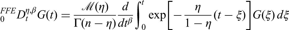
Let $G(t)$ be a continuous and fractal-differentiable function of order $\eta$ on the interval $(x,y)$ . The FF derivative of order $\eta$ with fractal dimension $\beta$ in the sense of the Riemann–Liouville formulation is defined as follows:

Using a power-law kernel:

$${}_0^{FFP}{D}_t^{\eta ,\beta }G(t)=\frac{1}{\mathrm{\Gamma }(n-\eta )}\frac{d}{d{t}^{\beta }}{\int }_0^t(t-\xi {)}^{n-\eta -1}G(\xi )d\xi$$

where $\eta >n-1$ , $\beta <n$ , and $n\in \mathbb{N}$ . Moreover, the fractal derivative is given by the following equation:

$$\frac{DG(\xi )}{D{\xi }^{\beta }}=\underset{t\to \xi }{lim}\frac{G(t)-G(\xi )}{t^{\beta }-{\xi }^{\beta }}$$

Using an exponential decay kernel:

$${}_0^{FFE}{D}_t^{\eta ,\beta }G(t)=\frac{\mathcal{M}(\eta )}{\mathrm{\Gamma }(n-\eta )}\frac{d}{d{t}^{\beta }}{\int }_0^t\exp [-\frac{\eta }{1-\eta }(t-\xi )]G(\xi )d\xi$$

where $\eta >0$ , $\beta \le n\in \mathbb{N}$ , and the normalization function satisfies $\mathcal{M}(0)=\mathcal{M}(1)=1$ .

Using a ML kernel:

$${}_0^{FFM}{D}_t^{\eta ,\beta }G(t)=\frac{\mathcal{A}\mathcal{B}(\eta )}{1-\eta }\frac{d}{d{t}^{\beta }}{\int }_0^t{E}_{\eta }[-\frac{\eta }{1-\eta }(t-\xi {)}^{\eta }]G(\xi )d\xi$$

where $\mathcal{A}\mathcal{B}(\eta )=1-\eta +\frac{\eta }{\mathrm{\Gamma }(\eta )}$ is the normalization function, $E_{\eta }(\cdot )$ denotes the ML function, and $0<\eta ,\beta \le 1$ .

Definition 2

Let $G(t)$ be continuous on $(x,y)$ with $0\le \eta ,\beta \le 1$ . The FF integral of $G(t)$ of order $\eta$ and fractal dimension $\beta$ is defined as follows:

With a power-law kernel:

$${}_0^{FFP}{I}^{\eta ,\beta }G(t)=\frac{1}{\mathrm{\Gamma }(\eta )}{\int }_0^t(t-\xi {)}^{\eta -1}{\xi }^{1-\beta }G(\xi )d\xi$$

With an exponential decay kernel:

$${}_0^{FFE}{I}^{\eta ,\beta }G(t)=\frac{\beta (1-\eta )t^{\beta -1}G(t)}{\mathcal{M}(\eta )}+\frac{\eta \beta }{\mathcal{M}(\eta )}{\int }_0^t{\xi }^{\eta -1}G(\xi )d\xi$$

With a ML kernel:

$${}_0^{FFM}{I}^{\eta ,\beta }G(t)=\frac{\beta (1-\eta )t^{\beta -1}G(t)}{\mathcal{A}\mathcal{B}(\eta )}+\frac{\eta \beta }{\mathcal{A}\mathcal{B}(\eta )\mathrm{\Gamma }(\eta )}{\int }_0^t(t-\xi {)}^{\eta -1}{\xi }^{\beta -1}G(\xi )d\xi$$

Novelty and contribution of the present work

The novelty of this study lies in developing a FF anthracnose disease model that incorporates both rain-splash transmission and plant hypersensitive response-two crucial but rarely combined biological mechanisms in existing models. Unlike previous integer-order or purely fractional models, the present work employs the FFO with a ML kernel to capture long-term memory and spatial heterogeneity effects inherent in fungal disease propagation. The study further conducts bifurcation and chaos analyses to reveal how environmental fluctuations and hypersensitive defense can drive transitions between stable and chaotic regimes. These findings go beyond earlier efforts by linking mathematical complexity with real biological behavior, offering new insights for optimizing control strategies such as fungicide timing and resistance management under varying rainfall conditions.

Formulation of anthracnose virus

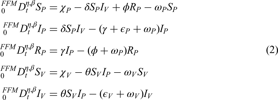
To describe the transmission of anthracnose under splashing-rain conditions, we first outline the biological process governing the interaction between healthy, infected, and removed plants. The model considers environmental factors such as rainfall, humidity, and the hypersensitive response (HR) mechanism. Healthy plants become infected through contact with spores dispersed by rain droplets, while HR restricts further spread by isolating infected cells. These biological interactions are then represented mathematically through a system of nonlinear differential equations.

This study proposes a new mathematical model for anthracnose dynamics that incorporates control measures considering various effects and the early detection of infected plants caused by splashing-rain transmission. To the best of our knowledge, no prior work has developed a model of this form. The proposed model considers distinct compartments for both plants and vectors, thereby capturing the complex interactions that drive the spread of anthracnose in agricultural environments.

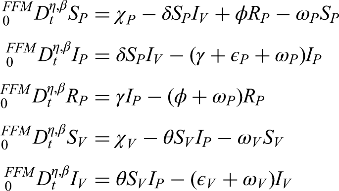
In the plant population, three classes are defined: susceptible plants ( $P_S$ ), infected plants subjected to hypersensitive response and phytosanitary practices ( $P_I$ ), and recovered plants ( $P_R$ ). Thus, the total plant population is expressed as follows:

$$N_P=P_S+P_I+P_R$$

The vector population, responsible for transmitting the bacterial anthracnose pathogen via splashing-rain mechanisms, is divided into two classes: susceptible vectors ( $S_V$ ) and infected vectors ( $I_V$ ). Hence, the total vector population is given by the following equation:

$$N_V=S_V+I_V$$

The size of the vector population $N_V$ is assumed constant, owing to the balance between immigration and emigration rates, while the plant population $N_P$ varies dynamically over time. Anthracnose transmission occurs in a non-circulative and non-persistent manner, without latency in either plant or vector populations. The rate at which healthy suckers are replanted balances the rate of roguing (removal) of diseased plants. Furthermore, a fraction of fertilized susceptible plants transitions into the protected plant class, whereas unfertilized susceptible plants remain vulnerable and may eventually move into the infected compartment.

The methodology of this study is based on the formulation and analysis of a nonlinear compartmental model describing the spread of anthracnose disease in plants under splashing-rain conditions. The model divides the total plant population into epidemiological compartments and integrates the FFO with the ML kernel to incorporate both memory and fractal effects in the disease dynamics. Analytical techniques are used to study the existence, uniqueness, boundedness, and stability of solutions through Lipschitz and linear growth conditions. Furthermore, bifurcation analysis is conducted to identify the transition from stable to oscillatory or chaotic behavior, while a two-step Lagrange polynomial scheme is applied for numerical approximation. Consensus on parameter values and control strategies is reached through iterative adjustment and comparison with reported biological patterns of anthracnose spread.

This compartmental model provides a robust basis for analyzing the dynamics of anthracnose spread and the role of control strategies in maintaining plant health.

The parameter values used in this study were selected based on relevant literature and biological reasoning. Parameters such as plant birth rate ( ${\chi }_P$ ), natural death rates ( ${\omega }_P,{\omega }_V$ ), and disease-induced death rates ( ${ϵ}_P,{ϵ}_V$ ) were adopted from similar fractional-order epidemiological models of plant–pathogen interactions.^8–10 The transmission rates ( $\delta$ , $\theta$ ) and recovery rate ( $\gamma$ ) were estimated to reflect typical anthracnose spread dynamics under splashing-rain conditions. Parameters ${\delta }_1=0.8$ , $\eta =0.3$ , $d_1=0.2$ , ${\delta }_2=0.05$ , $\xi =0.48$ , $\alpha =0.024$ , $\gamma =0.25$ , and $\beta =0.33$ were chosen to ensure system stability and realistic biological interpretation during numerical simulations. A sensitivity analysis was also conducted to confirm the robustness of these values.

Flowchart of the proposed anthracnose disease model showing the transitions among plant compartments. Each arrow represents the transmission pathway of infection through splashing rain, indicating how susceptible plants become infected and how hypersensitive response reduces further spread. Figure 1 illustrate the biological model of anthracnose spread, where rainfall-driven spore movement plays a key role. The compartments reflect healthy, infected, and resistant plants, emphasizing how environmental factors facilitate transmission.

$$\begin{array}{rl}D{S}_P& ={\chi }_P-\delta S_P{I}_V+\varphi R_P-{\omega }_P{S}_P\\ D{I}_P& =\delta S_P{I}_V-(\gamma +{ϵ}_P+{\omega }_P)I_P\\ D{R}_P& =\gamma I_P-(\varphi +{\omega }_P)R_P\\ D{S}_V& ={\chi }_V-\theta S_V{I}_P-{\omega }_V{S}_V\\ D{I}_V& =\theta S_V{I}_P-({ϵ}_V+{\omega }_V)I_V\end{array}$$

(1)

Figure 1.

The newly developed model is illustrated in the flowchart.

Figure 2.

Parameter estimation.

Figure 3.

Reproductive number graphs with different parameters. (a) $R_0$ with respect to $\theta$ ; (b) $R_0$ with respect to ${\chi }_P$ ; (c) $R_0$ with respect to ${\chi }_V$ ; (d) $R_0$ with respect to $\delta$ ; (e) $R_0$ with respect to ${\omega }_P$ ; (f) $R_0$ with respect to ${\omega }_V$ ; (g) $R_0$ with respect to ${ϵ}_P$ ; and (h) $R_0$ with respect to $\gamma$ .

Figure 4.

Reproductive number graphs with different parameters. (a) With respect to parameter $\theta$ and ${\chi }_P$ ; (b) with respect to parameter ${\chi }_P$ and ${\chi }_V$ ; (c) with respect to parameter ${\chi }_V$ and $\delta$ ; (d) with respect to parameter $\delta$ and $\varphi$ ; (e) with respect to parameter $\varphi$ and ${\omega }_P$ ; (f) with respect to parameter ${\omega }_P$ and ${\omega }_V$ ; (g) with respect to parameter ${\omega }_V$ and $\gamma$ ; (h) with respect to parameter $\gamma$ and ${ϵ}_P$ ; and (i) with respect to parameter ${ϵ}_P$ and $\theta$ .

initially set up as follows: $S_P(0)=S_P^0$ , $I_P(0)=I_P^0$ , $R_P(0)=R_P^0$ , $S_V(0)=S_V^0$ , and $I_V(0)=I_V^0$ .

One key assumption of this model is that the total vector population remains constant during the study period. This simplification allows for a clearer analysis of plant-pathogen interactions without introducing additional environmental complexity. Similar assumptions have been adopted in earlier works on plant disease modeling where vector fluctuations were minimal over short time scales.^8,9,19 However, in real conditions, vector populations are influenced by environmental factors such as rainfall and humidity, which promote spore dispersal and survival. Future extensions of this model may incorporate dynamic vector equations to better capture these environmental effects.

Using the notion of a FF derivative on the differential equation system above, we now obtain

$$\begin{array}{rl}{}_0^{FFM}{D}_t^{\eta ,\beta }{S}_P& ={\chi }_P-\delta S_P{I}_V+\varphi R_P-{\omega }_P{S}_P\\ {}_0^{FFM}{D}_t^{\eta ,\beta }{I}_P& =\delta S_P{I}_V-(\gamma +{ϵ}_P+{\omega }_P)I_P\\ {}_0^{FFM}{D}_t^{\eta ,\beta }{R}_P& =\gamma I_P-(\varphi +{\omega }_P)R_P\\ {}_0^{FFM}{D}_t^{\eta ,\beta }{S}_V& ={\chi }_V-\theta S_V{I}_P-{\omega }_V{S}_V\\ {}_0^{FFM}{D}_t^{\eta ,\beta }{I}_V& =\theta S_V{I}_P-({ϵ}_V+{\omega }_V)I_V\end{array}$$

(2)

In this instance, the FFO for ML is ${}_0^{FFM}{D}_t^{\eta ,\beta }$ , where $0<\eta \le 1$ and $0<\beta \le 1$ . The system under description is associated with the initial conditions $S_P(0)=S_P^0$ , $I_P(0)=I_P^0$ , $R_P(0)=R_P^0$ , $S_V(0)=S_V^0$ , and $I_V(0)=I_V^0$ .

The use of fractional calculus in this study is motivated by the inherent memory and hereditary characteristics observed in plant disease dynamics. In anthracnose infection, spores can persist on plant surfaces or in the soil for extended periods, and environmental conditions such as moisture and humidity influence delayed infection responses. Fractional-order operators capture these memory effects by considering the past states of the system in the current rate of change. This approach provides a more realistic description of disease progression compared to classical integer-order models, where such persistence and delayed effects are neglected.^14–16

Significance of exact and numerical solutions

The study of nonlinear differential equations is fundamental in applied mathematics, science, and engineering because such equations describe complex real-world phenomena that rarely admit simple analytical forms. Exact solutions, when obtainable, provide deep theoretical insights into the qualitative behavior of the system, such as equilibrium stability, threshold dynamics, and bifurcation structures. They serve as benchmarks for validating numerical schemes and help identify critical parameter regimes where system transitions occur.

However, due to the inherent nonlinearity and memory effects introduced by FFOs, exact analytical solutions are often difficult or impossible to derive. In such cases, numerical approaches become essential tools for exploring system behavior under realistic biological and environmental conditions. Numerical simulations allow researchers to visualize transient dynamics, compare fractional and integer-order responses, and investigate the influence of parameter variations on disease progression. Therefore, the combination of exact and numerical analyses not only strengthens the mathematical rigor of the proposed model but also enhances its applicability to real anthracnose management by providing predictive and computational tools for decision-making.

Methodology and data fitting approach

In this study, the proposed anthracnose transmission model was developed through a systematic process combining biological evidence, literature consensus, and mathematical reasoning. The compartmental structure was formulated based on previously established fungal disease models that account for susceptible, infected, and recovered plant and vector populations. Expert consensus and published epidemiological studies on anthracnose and related plant-fungal systems were consulted to validate the inclusion of key biological interactions such as rain-splash transmission, hypersensitive response, and recovery mechanisms. The transition from integer-order to fractal-fractional formulations was adopted to capture memory-dependent effects observed in anthracnose persistence under variable environmental conditions. The fitting procedure minimized the sum of squared errors between model outputs (infected plant population) and observed data points, yielding optimized parameter estimates for transmission rates $(\delta ,\theta )$ and recovery rate $(\gamma )$ . The resulting fitted curves demonstrated strong agreement with empirical patterns, supporting the model’s validity and its capacity to reproduce realistic anthracnose dynamics shown in Figure 2.

Model reproduction number and equilibrium points

In this section, we derive the equilibrium states of the proposed anthracnose model (2). Two types of equilibria are obtained: the disease-free equilibrium (DFE) and the endemic equilibrium (EE).

The DFE, where the infection is completely absent in both the plant and vector populations, is given by the following equation:

$$E_1=(S_P\to \frac{{\chi }_P}{{\omega }_P},I_P\to 0,R_P\to 0,S_V\to \frac{{\chi }_V}{{\omega }_V},I_V\to 0)$$

The EE, where anthracnose persists in the system, is denoted by the following equation:

$$E_2=(S_P*,I_P*,R_P*,S_V*,I_V*)$$

where each state variable assumes a positive steady-state value in the presence of infection.

$$\begin{array}{rl}{S}_P*& =\frac{({\omega }_V+{ϵ}_V)(\gamma +{\omega }_P+{ϵ}_P)(\theta {\chi }_P({\omega }_P+\varphi )+{\omega }_V(\gamma {\omega }_P+({\omega }_P+{ϵ}_P)({\omega }_P+\varphi )))}{\theta ({\omega }_P(\delta {\chi }_V(\gamma +{\omega }_P+\varphi )+{ϵ}_V(\gamma +{\omega }_P)({\omega }_P+\varphi )+{\omega }_V(\gamma +{\omega }_P)({\omega }_P+\varphi ))+{ϵ}_P({\omega }_P+\varphi )({\omega }_P({\omega }_V+{ϵ}_V)+\delta {\chi }_V))}\\ I_P*& =-\frac{({\omega }_P+\varphi )({\omega }_P{\omega }_V({\omega }_V+{ϵ}_V)(\gamma +{\omega }_P+{ϵ}_P)-\delta \theta {\chi }_P{\chi }_V)}{\theta ({\omega }_P(\delta {\chi }_V(\gamma +{\omega }_P+\varphi )+{ϵ}_V(\gamma +{\omega }_P)({\omega }_P+\varphi )+{\omega }_V(\gamma +{\omega }_P)({\omega }_P+\varphi ))+{ϵ}_P({\omega }_P+\varphi )({\omega }_P({\omega }_V+{ϵ}_V)+\delta {\chi }_V))}\\ R_P*& =\frac{\gamma \delta \theta {\chi }_P{\chi }_V-\gamma {\omega }_P{\omega }_V({\omega }_V+{ϵ}_V)(\gamma +{\omega }_P+{ϵ}_P)}{\theta ({\omega }_P(\delta {\chi }_V(\gamma +{\omega }_P+\varphi )+{ϵ}_V(\gamma +{\omega }_P)({\omega }_P+\varphi )+{\omega }_V(\gamma +{\omega }_P)({\omega }_P+\varphi ))+{ϵ}_P({\omega }_P+\varphi )({\omega }_P({\omega }_V+{ϵ}_V)+\delta {\chi }_V))}\\ S_V*& =\frac{{\omega }_P(\delta {\chi }_V(\gamma +{\omega }_P+\varphi )+{ϵ}_V(\gamma +{\omega }_P)({\omega }_P+\varphi )+{\omega }_V(\gamma +{\omega }_P)({\omega }_P+\varphi ))+{ϵ}_P({\omega }_P+\varphi )({\omega }_P({\omega }_V+{ϵ}_V)+\delta {\chi }_V)}{\delta (\theta {\chi }_P({\omega }_P+\varphi )+{\omega }_V(\gamma {\omega }_P+({\omega }_P+{ϵ}_P)({\omega }_P+\varphi )))}\\ I_V*& =\frac{({\omega }_P+\varphi )(\delta \theta {\chi }_P{\chi }_V-{\omega }_P{\omega }_V({\omega }_V+{ϵ}_V)(\gamma +{\omega }_P+{ϵ}_P))}{\delta ({\omega }_V+{ϵ}_V)(\theta {\chi }_P({\omega }_P+\varphi )+{\omega }_V(\gamma {\omega }_P+({\omega }_P+{ϵ}_P)({\omega }_P+\varphi )))}\end{array}$$

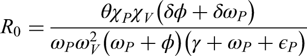
Reproductive number is

$$R_0=\frac{\theta {\chi }_P{\chi }_V(\delta \varphi +\delta {\omega }_P)}{{\omega }_P{\omega }_V^2({\omega }_P+\varphi )(\gamma +{\omega }_P+{ϵ}_P)}$$

Sensitivity analysis

Sensitivity analysis is useful for understanding how different conditions, especially those involving uncertain data, impact a model’s stability. It also helps identify important process variables. For instance, by calculating the partial derivatives of the threshold with respect to relevant parameters, we can assess the sensitivity of $R_0$ as follows:

$$\frac{\mathrm{\partial }{R}_0}{\mathrm{\partial }\theta }=\frac{{\chi }_P{\chi }_V(\delta \varphi +\delta {\omega }_P)}{{\omega }_P{\omega }_V^2({\omega }_P+\varphi )(\gamma +{\omega }_P+{ϵ}_P)}>0$$

$$\begin{array}{rl}\frac{\mathrm{\partial }{R}_0}{\mathrm{\partial }{\chi }_P}& =\frac{\theta {\chi }_V(\delta \varphi +\delta {\omega }_P)}{{\omega }_P{\omega }_V^2({\omega }_P+\varphi )(\gamma +{\omega }_P+{ϵ}_P)}>0\\ \frac{\mathrm{\partial }{R}_0}{\mathrm{\partial }{\chi }_V}& =\frac{\theta {\chi }_P(\delta \varphi +\delta {\omega }_P)}{{\omega }_P{\omega }_V^2({\omega }_P+\varphi )(\gamma +{\omega }_P+{ϵ}_P)}>0\end{array}$$

$$\begin{array}{rl}\frac{\mathrm{\partial }{R}_0}{\mathrm{\partial }\delta }& =\frac{\theta {\chi }_P{\chi }_V}{{\omega }_P{\omega }_V^2(\gamma +{\omega }_P+{ϵ}_P)}>0\\ \frac{\mathrm{\partial }{R}_0}{\mathrm{\partial }\varphi }& =\frac{\delta \theta {\chi }_P{\chi }_V}{{\omega }_P{\omega }_V^2({\omega }_P+\varphi )(\gamma +{\omega }_P+{ϵ}_P)}-\frac{\theta {\chi }_P{\chi }_V(\delta \varphi +\delta {\omega }_P)}{{\omega }_P{\omega }_V^2{({\omega }_P+\varphi )}^2(\gamma +{\omega }_P+{ϵ}_P)}>0\end{array}$$

$$\begin{array}{rl}\frac{\mathrm{\partial }{R}_0}{\mathrm{\partial }{\omega }_P}& =-\frac{\delta \theta {\chi }_P{\chi }_V(\gamma +2{\omega }_P+{ϵ}_P)}{{\omega }_P^2{\omega }_V^2{(\gamma +{\omega }_P+{ϵ}_P)}^2}<0\\ \frac{\mathrm{\partial }{R}_0}{\mathrm{\partial }\gamma }& =-\frac{\theta {\chi }_P{\chi }_V(\delta \varphi +\delta {\omega }_P)}{{\omega }_P{\omega }_V^2({\omega }_P+\varphi ){(\gamma +{\omega }_P+{ϵ}_P)}^2}<0\end{array}$$

$$\begin{array}{rl}\frac{\mathrm{\partial }{R}_0}{\mathrm{\partial }{ϵ}_P}& =-\frac{\theta {\chi }_P{\chi }_V(\delta \varphi +\delta {\omega }_P)}{{\omega }_P{\omega }_V^2({\omega }_P+\varphi ){(\gamma +{\omega }_P+{ϵ}_P)}^2}<0\\ \frac{\mathrm{\partial }{R}_0}{\mathrm{\partial }{\omega }_V}& =-\frac{2\theta {\chi }_P{\chi }_V(\delta \varphi +\delta {\omega }_P)}{{\omega }_P{\omega }_V^3({\omega }_P+\varphi )(\gamma +{\omega }_P+{ϵ}_P)}<0\end{array}$$

It is important to note that adjusting the settings can significantly affect the value of $R_0$ . In our study, parameters like $\gamma$ , ${\omega }_P$ , ${\omega }_V$ , and ${ϵ}_P$ represent expansion, while $\theta ,$ ${\chi }_P,$ ${\chi }_V$ , $\delta$ , and $\varphi$ signify contraction. Therefore, it is essential to prioritize prevention over treatment for effective infection control.

It is evident from all of the aforementioned subfigures that the value of $R_0$ is very responsive in terms of how its rate of change behaves. The behavior of $R_0$ w.r.t ${\chi }_P\mathrm{\&}\theta$ , ${\chi }_V\mathrm{\&}{\delta }_2$ , and ${\chi }_P\mathrm{\&}{\chi }_V$ is approximately similar with minor effects at these parameters. Similarly, the behavior of $R_0$ w.r.t ${\omega }_P\mathrm{\&}{\omega }_V$ , ${\omega }_V\mathrm{\&}\gamma$ , and $\gamma \mathrm{\&}{ϵ}_P$ approximately same behavior with some minor effects. Furthermore, the behavior of $R_0$ w.r.t $\delta \mathrm{\&}\varphi$ , $\varphi \mathrm{\&}{\omega }_P$ , and ${ϵ}_P\mathrm{\&}\theta$ having approximately different behavior with minor effects. On the other hand, every subfigure indicates that the rate of change of every parameter is bounded, which is essential for stable conditions shown in Figures 3 and 4.

Examining the local stability on equilibrium points

We now present theorems and corresponding proofs that establish the local stability properties of the equilibrium points of the proposed fractional-order anthracnose model.

Theorem 1

The fractional-order anthracnose model is locally asymptotically stable at the DFE if the basic reproduction number $R_0<1$ . Conversely, the DFE becomes unstable whenever $R_0>1$ .

Proof.

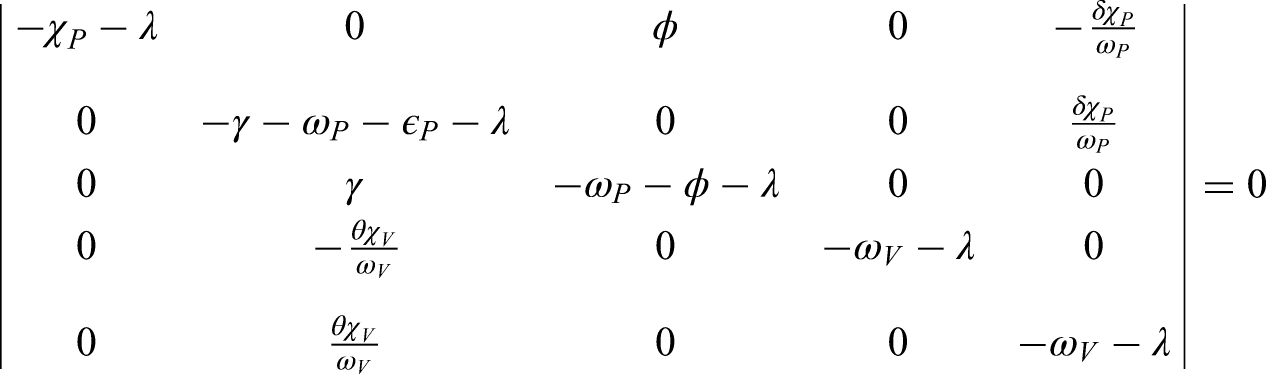
To analyze the local stability of the system at its equilibrium points, we consider the Jacobian matrix $J$ associated with the model (2). By evaluating $J$ at the disease-free equilibrium $E_1$ , we obtain the characteristic polynomial that governs the local dynamics of the system.

The eigenvalues of $J$ determine the stability of the DFE. If all eigenvalues of $J$ have negative real parts, the equilibrium is locally asymptotically stable. Standard linear stability theory for fractional-order systems states that the disease-free equilibrium is stable provided that

$$|\arg ({\lambda }_i)|>\frac{\eta \pi }{2},\mathrm{\forall }{\lambda }_i\in \sigma (J)$$

where $\sigma (J)$ denotes the spectrum of $J$ and $\eta$ is the fractional order.

It follows that the stability condition is directly linked to the basic reproduction number $R_0$ . In particular, if $R_0<1$ , all eigenvalues satisfy the above stability criterion, and hence the DFE is locally asymptotically stable. On the other hand, when $R_0>1$ , at least one eigenvalue violates the condition, leading to instability of the DFE.

$$\begin{array}{r}J|E(S_P{I}_P{R}_P{S}_V{I}_V)=\left(\begin{array}{ccccc}-{\chi }_P& 0& \varphi & 0& -\delta S_P\\ 0& -\gamma -{\omega }_P-{ϵ}_P& 0& 0& \delta S_P\\ 0& \gamma & -{\omega }_P-\varphi & 0& 0\\ 0& -\theta S_V& 0& -{\omega }_V& 0\\ 0& \theta S_V& 0& 0& -{\omega }_V\end{array}\right)\end{array}$$

At $E(P_{S}000S_v{I}_v)=\{\frac{{\chi }_P}{{\omega }_P},0,0,\frac{{\chi }_P}{{\omega }_P},0\}$ the Jacobian matrix becomes

$$\begin{array}{r}J|E(S_{P}00S_{V}0)=\left(\begin{array}{ccccc}-{\chi }_P& 0& \varphi & 0& -\frac{\delta {\chi }_P}{{\omega }_P}\\ 0& -\gamma -{\omega }_P-{ϵ}_P& 0& 0& \frac{\delta {\chi }_P}{{\omega }_P}\\ 0& \gamma & -{\omega }_P-\varphi & 0& 0\\ 0& -\frac{\theta {\chi }_V}{{\omega }_V}& 0& -{\omega }_V& 0\\ 0& \frac{\theta {\chi }_V}{{\omega }_V}& 0& 0& -{\omega }_V\end{array}\right)\end{array}$$

For the characteristic equation

$$|J_0-\lambda I|=0$$

$$\begin{array}{r}\left|\begin{array}{ccccc}-{\chi }_P-\lambda & 0& \varphi & 0& -\frac{\delta {\chi }_P}{{\omega }_P}\\ 0& -\gamma -{\omega }_P-{ϵ}_P-\lambda & 0& 0& \frac{\delta {\chi }_P}{{\omega }_P}\\ 0& \gamma & -{\omega }_P-\varphi -\lambda & 0& 0\\ 0& -\frac{\theta {\chi }_V}{{\omega }_V}& 0& -{\omega }_V-\lambda & 0\\ 0& \frac{\theta {\chi }_V}{{\omega }_V}& 0& 0& -{\omega }_V-\lambda \end{array}\right|=0\end{array}$$

Matrix with the characteristic equation is

$$\frac{(\lambda +{\chi }_P)(\lambda +{\omega }_V)(-\lambda -{\omega }_P-\varphi )({\omega }_P{\omega }_V(\lambda +{\omega }_V)(\gamma +\lambda +{\omega }_P+{ϵ}_P)-\delta \theta {\chi }_P{\chi }_V)}{{\omega }_P{\omega }_V}=0$$

The determinant matrix $(\lambda )$ can be solved to get the following eigenvalues:

$$\lambda =-{\chi }_P$$

(3)

$$\begin{array}{rl}\lambda & =-{\omega }_P-\varphi \\ \lambda & =-{\omega }_V\\ \lambda & =\frac{-\gamma {\omega }_P{\omega }_V+{\omega }_P^2(-{\omega }_V)-{\omega }_P{\omega }_V^2-{\omega }_P{ϵ}_P{\omega }_V}{2{\omega }_P{\omega }_V}\\ \lambda & =-\frac{\gamma {\omega }_P{\omega }_V+{\omega }_P^2{\omega }_V+{\omega }_P{\omega }_V^2+{\omega }_P{ϵ}_P{\omega }_V}{2{\omega }_P{\omega }_V}\end{array}$$

The system is locally asymptotically stable since all eigenvalues of the Jacobian associated with system (2) possess negative real parts.

Evaluation of the proposed model

Positivity and boundedness of solutions

To ensure the biological relevance of the model, it is necessary to verify that the solutions remain positive and bounded for all $t>0$ . We assume that the conditions guaranteeing positivity of the solutions are satisfied under realistic parameter values. These conditions are then analyzed to establish their validity and the admissible limits of the system. Accordingly, we obtain the following results:

$$\begin{array}{rl}{I}_P(t)& \ge I_P(0)e^{-(\gamma +{ϵ}_P+{\omega }_P)t},\mathrm{\forall }t\ge 0\\ R_P(t)& \ge R_P(0)e^{-(\varphi +{\omega }_P)t},\mathrm{\forall }t\ge 0\\ I_V(t)& \ge I_V(0)e^{-({ϵ}_V+{\omega }_V)t},\mathrm{\forall }t\ge 0\end{array}$$

Let $D_X$ represent $X$ ’s domain. Describe the standard

$$\Vert X{\Vert }_{\mathrm{\infty }}=\underset{t\in D_X}{sup}|X(t)|$$

With this norm, the function $P_S(t)$ has;

$$\begin{array}{rl}{}_0^{FFM}{D}_t^{\eta ,\beta }{S}_P& ={\chi }_P-\delta S_P{I}_V+\varphi R_P-{\omega }_P{S}_P\\ & \ge -(\delta I_V+{\omega }_P)S_P\ge -(\delta \underset{t\in D_{I_V}}{sup}{I}_V+{\omega }_P)S_P=-(\delta \Vert I_V{\Vert }_{\mathrm{\infty }}+{\omega }_P)S_P\end{array}$$

For ordinary derivative, we have

$$S_P(t)=S_P(0)e^{-(\delta \Vert I_V{\Vert }_{\mathrm{\infty }}+{\omega }_P)t},\mathrm{\forall }t\ge 0$$

Similarly, for $S_V$ , we have

$$\begin{array}{rl}{}_0^{FFM}{D}_t^{\eta ,\beta }{S}_V& ={\chi }_V-\theta S_V{I}_P-{\omega }_V{S}_V\\ & \ge -(\theta I_P+{\omega }_V)S_V\ge -(\theta \underset{t\in D_{I_P}}{sup}{I}_P+{\omega }_V)S_V=-(\theta \Vert I_P{\Vert }_{\mathrm{\infty }}+{\omega }_V)S_V\end{array}$$

For ordinary derivative, we have

$$S_V(t)=S_V(0)e^{-(\theta \Vert I_P{\Vert }_{\mathrm{\infty }}+{\omega }_V)t},\mathrm{\forall }t\ge 0$$

Positive solutions obtained through the use of non-local operators are presented below.

Positivity of solutions under non-local operators

If the initial conditions are non-negative, then all solutions of system (2) involving non-local operators remain positive. ¹⁶

$\bullet$ In the case of the FFO with a power-law kernel, we have

$$X(t)\ge 0,\mathrm{\forall }t\ge 0$$

which ensures the biological feasibility of the model

$$\begin{array}{rl}{S}_P(t)& \ge S_P(0)E_{\eta }(-{\phi }^{1-\beta }(\delta \Vert I_V{\Vert }_{\mathrm{\infty }}+{\omega }_P)t^{\eta })\\ I_P(t)& \ge I_P(0)E_{\eta }(-{\phi }^{1-\beta }(\gamma +{ϵ}_P+{\omega }_P)t^{\eta })\\ R_P(t)& \ge R_P(0)E_{\eta }(-{\phi }^{1-\beta }(\varphi +{\omega }_P)t^{\eta })\\ S_V(t)& \ge S_V(0)E_{\eta }(-{\phi }^{1-\beta }(\theta \Vert I_P{\Vert }_{\mathrm{\infty }}+{\omega }_V)t^{\eta })\\ I_V(t)& \ge I_V(0)E_{\eta }(-{\phi }^{1-\beta }({ϵ}_V+{\omega }_V)t^{\eta })\end{array}$$

where the time component is $\phi$ .

• For a FFO with an exponential kernel, we find $\mathrm{\forall }t\ge 0$ .

$$\begin{array}{rl}{S}_P(t)& \ge S_P(0)\exp (-\frac{{\chi }^{1-\beta }\eta (\delta \Vert I_V{\Vert }_{\mathrm{\infty }}+{\omega }_P)t}{\mathcal{M}(\eta )-(1-\eta )[\delta \Vert I_V{\Vert }_{\mathrm{\infty }}+{\omega }_P]})\\ I_P(t)& \ge I_P(0)\exp (-\frac{{\chi }^{1-\beta }\eta (\gamma +{ϵ}_P+{\omega }_P)t}{\mathcal{M}(\eta )-(1-\eta )[\gamma +{ϵ}_P+{\omega }_P]})\\ R_P(t)& \ge R_P(0)\exp (-\frac{{\chi }^{1-\beta }\eta (\varphi +{\omega }_P)t}{\mathcal{M}(\eta )-(1-\eta )[(\varphi +{\omega }_P)]})\\ S_V(t)& \ge S_V(0)\exp (-\frac{{\chi }^{1-\beta }\eta (\theta \Vert I_P{\Vert }_{\mathrm{\infty }}+{\omega }_V)t}{\mathcal{M}(\eta )-(1-\eta )[\theta \Vert I_P{\Vert }_{\mathrm{\infty }}+{\omega }_V]})\\ I_V(t)& \ge I_V(0)\exp (-\frac{{\chi }^{1-\beta }\eta ({ϵ}_V+{\omega }_V)t}{\mathcal{M}(\eta )-(1-\eta )[{ϵ}_V+{\omega }_V]})\end{array}$$

• We obtain $\mathrm{\forall }t\ge 0$ using a ML kernel for the FFO.

$$\begin{array}{rl}{S}_P(t)& \ge S_P(0)E_{\eta }(-\frac{{\chi }^{1-\beta }\eta (\delta \Vert I_V{\Vert }_{\mathrm{\infty }}+{\omega }_P)t}{\mathcal{A}\mathcal{B}(\eta )-(1-\eta )[\delta \Vert I_V{\Vert }_{\mathrm{\infty }}+{\omega }_P]})\\ I_P(t)& \ge I_P(0)E_{\eta }(-\frac{{\chi }^{1-\beta }\eta (\gamma +{ϵ}_P+{\omega }_P)t}{\mathcal{A}\mathcal{B}(\eta )-(1-\eta )[\gamma +{ϵ}_P+{\omega }_P]})\\ R_P(t)& \ge R_P(0)E_{\eta }(-\frac{{\chi }^{1-\beta }\eta (\varphi +{\omega }_P)t}{\mathcal{A}\mathcal{B}(\eta )-(1-\eta )[\varphi +{\omega }_P]})\\ S_V(t)& \ge S_V(0)E_{\eta }(-\frac{{\chi }^{1-\beta }\eta (\theta \Vert I_P{\Vert }_{\mathrm{\infty }}+{\omega }_V)t}{\mathcal{A}\mathcal{B}(\eta )-(1-\eta )[\theta \Vert I_P{\Vert }_{\mathrm{\infty }}+{\omega }_V]})\\ I_V(t)& \ge I_V(0)E_{\eta }(-\frac{{\chi }^{1-\beta }\eta ({ϵ}_V+{\omega }_V)t}{\mathcal{A}\mathcal{B}(\eta )-(1-\eta )[{ϵ}_V+{\omega }_V]})\end{array}$$

Positively invariant region

Lemma 1

Define

$${\mathrm{\Psi }}^P=\{(S_P,I_P,R_P)\in {\mathbb{R}}_{+}^3:0\le N_P(t)\le \frac{{\chi }_P}{{\omega }_P}\}$$

(4)

$${\mathrm{\Psi }}^V=\{(S_V,I_V)\in {\mathbb{R}}_{+}^2:0\le N_V(t)\le \frac{{\chi }_V}{{\omega }_V}\}$$

(5)and let

$$\mathrm{\Psi }={\mathrm{\Psi }}^P\times {\mathrm{\Psi }}^V$$

For non-negative initial conditions, the region $\mathrm{\Psi }$ attracts all solutions of the proposed system in ${\mathbb{R}}_{+}^5$ , provided that

$$N_P(0)\le \frac{{\chi }_P}{{\omega }_P},N_V(0)\le \frac{{\chi }_V}{{\omega }_V}$$

Proof.

We now establish that system (2) admits positive solutions, and the details are as follows:

$$\begin{array}{rl}{}_0^{FFM}{D}_t^{\eta ,\beta }{S}_P{|}_{S_P=0}& ={\chi }_P+\varphi R_P\ge 0\\ {}_0^{FFM}{D}_t^{\eta ,\beta }{I}_P{|}_{I_P=0}& =\delta S_P{I}_V\ge 0\\ {}_0^{FFM}{D}_t^{\eta ,\beta }{R}_P{|}_{R_P=0}& =\gamma I_P\ge 0\\ {}_0^{FFM}{D}_t^{\eta ,\beta }{S}_V{|}_{S_V=0}& ={\chi }_V\ge 0\\ {}_0^{FFM}{D}_t^{\eta ,\beta }{I}_V{|}_{I_V=0}& =\theta S_V{I}_P\ge 0\end{array}$$

(6)According to the system (6), the area ${\mathbb{R}}_{+}^5$ contains the vector field for each hyperplane that includes the non-negative orthant with $t\ge 0$ . The entire population is as follows once the component parts of the human population are included in model (2):

$$\begin{array}{rl}{}_0^{FFM}{D}_t^{\eta ,\beta }{N}_P(t)& ={\chi }_P-{\omega }_P(S_P+I_P+R_P)-{ϵ}_P{I}_P\\ & \ge {\chi }_P-{\omega }_P(S_P+I_P+R_P)={\chi }_P-{\omega }_P{N}_P\end{array}$$

We also write as follows:

$${}_0^{FFM}{D}_t^{\eta ,\beta }{N}_P(t)\le {\chi }_P-{\omega }_P{N}_P$$

Suppose that $N_P(0)\le \frac{{\chi }_P}{{\omega }_P}$

$$\Rightarrow N_P(t)\le \frac{{\chi }_P}{{\omega }_P}$$

Similarly for bacterial population

$${}_0^{FFM}{D}_t^{\eta ,\beta }{N}_V(t)={\chi }_V-{\omega }_V(S_V+I_V)-{ϵ}_V{I}_V\ge {\chi }_V-{\omega }_V(S_V+I_V)={\chi }_V-{\omega }_V{N}_V$$

We also write as follows:

$${}_0^{FFM}{D}_t^{\eta ,\beta }{N}_V(t)\le {\chi }_V-{\omega }_V{N}_V$$

Suppose that $N_V(0)\le \frac{{\chi }_V}{{\omega }_V}$

$$\Rightarrow N_V(t)\le \frac{{\chi }_V}{{\omega }_V}$$

Consequently, for any $t>-0$ , a solution of the fractional model (2) survives in $\mathrm{\Psi }$ . This indicates that the closed set $\mathrm{\Psi }$ is positively invariant for the fractional model. Consequently, our model (2) may be investigated inside the feasible region:

$$\mathrm{\Psi }=\{(S_P,I_P,R_P,S_V,I_V)\in {\mathbb{R}}_{+}^5:0<N_P(t)\le \frac{{\chi }_P}{{\omega }_P},0<N_V(t)\le \frac{{\chi }_V}{{\omega }_V}\}$$

Flip bifurcation analysis

In this section, we employ bifurcation theory^24–26 to analyze the possibility of a flip bifurcation at the equilibrium point

$$E=(\frac{{\chi }_P}{{\omega }_P},0,0,\frac{{\chi }_V}{{\omega }_V},0)$$

Analysis of bifurcation at the equilibrium points of the anthracnose model.

Computation of the eigenvalues reveals that none of them equals $\pm 1$ , suggesting the potential occurrence of a flip bifurcation within the system. The parameter set is denoted by the following equation:

$$(\varphi ,{\chi }_P,{\chi }_V,{\omega }_P,{\omega }_V,\delta ,\gamma ,{ϵ}_P,{ϵ}_V)$$

At the equilibrium $E_1$ , we have

$$F|E_1=\{(\varphi ,{\chi }_P,{\chi }_V,{\omega }_P,{\omega }_V,\delta ,\gamma ,{ϵ}_P,{ϵ}_V):{\omega }_P=\frac{\varphi }{2},{\omega }_V=0\}$$

(6)

The following theorem formally establishes the non-existence of a flip bifurcation for system (2) at the specified parameter set.

Theorem 2

Consider system (2) with respect to the parameter set

$$(\varphi ,{\chi }_P,{\chi }_V,{\omega }_P,{\omega }_V,\delta ,\gamma ,{ϵ}_P,{ϵ}_V)\in F(E_1)$$

Then, the system does not exhibit a flip bifurcation.

Proof.

To investigate the bifurcation behavior, we restrict system (2) to the invariant manifold defined by $I_P=R_P=I_V=0$ . This reduction yields the following simplified system, which forms the basis for further bifurcation analysis:

$$S_P^{t+1}={\chi }_P-{\omega }_P{S}_P$$

(7)

$$S_V^{t+1}={\chi }_V-{\omega }_V{S}_V$$

(8)From equation (7), one denotes map

$$f(S_P)={\chi }_P-{\omega }_P{S}_P$$

(9)

$$g(S_V)={\chi }_V-{\omega }_V{S}_V$$

(10)Now if ${\omega }_P={\omega }_P*=\frac{\varphi }{2},{\omega }_V={\omega }_V*=0$ , and $S_P=S_P*=\frac{{\chi }_P}{{\omega }_P},S_V=S_V*=\frac{{\chi }_V}{{\omega }_V}$ then from equation (9) we get

$$\frac{\mathrm{\partial }f}{\mathrm{\partial }{S}_P}=-{\omega }_P=-\frac{\varphi }{2}\ne 0$$

(11)

$$\frac{\mathrm{\partial }g}{\mathrm{\partial }{S}_V}=-({\omega }_V)=0$$

(12)

$$\frac{\mathrm{\partial }f}{\mathrm{\partial }{\omega }_P}=-S_P=-\frac{{\chi }_P}{{\omega }_P}$$

(13)

$$\frac{\mathrm{\partial }g}{\mathrm{\partial }{\omega }_V}=-S_V=-\frac{{\chi }_V}{{\omega }_V}$$

(14)and

$$\frac{{\mathrm{\partial }}^{2}f}{\mathrm{\partial }{S}_P^2}=0$$

(15)

$$\frac{{\mathrm{\partial }}^{2}f}{\mathrm{\partial }{S}_V^2}=0$$

(16)The above computations demonstrate that model 2 does not exhibit a flip bifurcation at $E_1$ , since the parametric condition (16) fails to satisfy the non-degeneracy requirement for

$$(\varphi ,{\chi }_P,{\chi }_V,{\omega }_P,{\omega }_V,\delta ,\gamma ,{ϵ}_P,{ϵ}_V)\in F(E_1)$$

Bifurcation diagrams showing the effect of key parameters $\delta$ and $\gamma$ on disease dynamics. Variations in $\delta$ (infection rate by splashing rain) and $\gamma$ (rate of hypersensitive response) determine whether the system remains stable or enters oscillatory/chaotic behavior, reflecting how changes in rainfall or plant resistance influence infection control. As shown in Figure 5, increasing $\delta$ amplifies disease transmission due to higher rain-induced spore dispersal, while increasing $\gamma$ enhances plant resistance, reducing infection prevalence. These results provide insight into how adjusting environmental conditions or applying control strategies (e.g. fungicide timing) could stabilize disease levels.

Figure 5.

Bifurcation graphs. (a) $S_P$ under parameter $\varphi$ ; (b) $S_P$ under parameter ${\omega }_P$ ; (c) $I_P$ under parameter $\delta$ ; (d) $I_P$ under parameter $\gamma$ ; (e) $R_P$ under parameter $\gamma$ ; (f) $R_P$ under parameter ${\omega }_P$ ; (g) $S_V$ under parameter $\theta$ ; (h) $S_V$ under parameter ${\omega }_V$ ; (i) $I_V$ under parameter ${\omega }_V$ ; and (j) $I_V$ under parameter $\theta$ .

The proposed model investigates recovery strategies through fungicide treatment for anthracnose disease. It is formulated as a continuous time-dependent system, capturing the complex impacts of the disease on trees. Based on the model assumptions, the following parameter values are considered: ${\delta }_1=0.8,$ $\eta =0.3,$ $d_1=0.2,$ ${\delta }_2=0.05,$ $\xi =0.48,$ $\alpha =0.024,$ $\gamma =0.25,$ and $\beta =0.33$ . The stability and boundedness of the system, as illustrated in Figure 2, are established using the linearization technique. Furthermore, a bifurcation diagram of the continuous-time model is constructed with respect to varying parameter ranges, such as ${\delta }_1\in [0,1]$ . Incorporating fungicide-based recovery measures allows the determination of stable states within the continuous model. Figure 2 also presents time-steady graphs that depict the variation of parameter values with respect to the overall requirement rate, thereby validating our theoretical results.

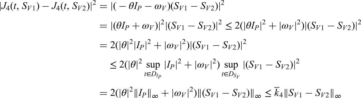
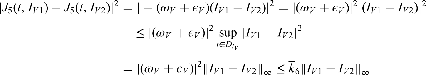
Effects of global derivatives on solution uniqueness and existence

The Riemann-Stieltjes integral is widely recognized as one of the most commonly employed integrals in the literature. For instance, consider

$$Z(a)=\int Z(a)dx$$

This can be extended in the Riemann-Stieltjes sense as follows:

$$Z_g(a)=\int Z(a)dgx$$

With respect to $g(a)$ , the global derivative of $z(a)$ is defined as follows:

$$D_{g}z(a)=\underset{h\to 0}{lim}\frac{z(a+h)-z(a)}{g(a+h)-g(a)}$$

In the case where both the numerator and denominator diverge, the expression reduces to

$$D_{g}z(a)=\underset{h\to 0}{lim}\frac{z^{\prime }(a)}{g^{\prime }(a)}$$

Since $g^{\prime }(a)\ne 0$ , the global derivative can replace the classical derivative for all $a\in {\mathbb{D}}_g^{\prime }$ , allowing us to study its effect on the dynamics of the maize foliar virus.

$$\begin{array}{rl}{D}_g{S}_P& ={\chi }_P-\delta S_P{I}_V+\varphi R_P-{\omega }_P{S}_P\\ D_g{I}_P& =\delta S_P{I}_V-(\gamma +{ϵ}_P+{\omega }_P)I_P\\ D_g{R}_P& =\gamma I_P-(\varphi +{\omega }_P)R_P\\ D_g{S}_V& ={\chi }_V-\theta S_V{I}_P-{\omega }_V{S}_V\\ D_g{I}_V& =\theta S_V{I}_P-({ϵ}_V+{\omega }_V)I_V\end{array}$$

For hygienic reasons, let’s suppose that $g$ is differentiable.

$$\begin{array}{rl}{S}_P^{\prime }& =g^{\prime }[{\chi }_P-\delta S_P{I}_V+\varphi R_P-{\omega }_P{S}_P]\\ I_P^{\prime }& =g^{\prime }[\delta S_P{I}_V-(\gamma +{ϵ}_P+{\omega }_P)I_P]\\ R_P^{\prime }& =g^{\prime }[\gamma I_P-(\varphi +{\omega }_P)R_P]\\ S_V^{\prime }& =g^{\prime }[{\chi }_V-\theta S_V{I}_P-{\omega }_V{S}_V]\\ I_V^{\prime }& =g^{\prime }[\theta S_V{I}_P-({ϵ}_V+{\omega }_V)I_V]\end{array}$$

Proper selection of the function $g$ will yield a certain outcome. For instance, if $g=t^{\kappa }$ , where $\kappa$ is a real number, fractal movement will be observed. The circumstances for our action were

$$\Vert g^{\prime }{\Vert }_{\mathrm{\infty }}=\underset{t\in D_g^{\prime }}{sup}g<N$$

where

$$\zeta =S_P,I_P,R_P,S_V,I_V$$

The two conditions listed below must be verified.

1. $|J(t,S_P,I_P,R_P,S_V,I_V)|<K(1+|S_P{|}^2)$

2. $\mathrm{\forall }{S}_{P1},S_{P2}$ , we have

   $$\Vert J(t,S_{P1},I_P,R_P,S_V,I_V)-J(t,S_{P2},I_P,R_P,S_V,I_V)\Vert <k\Vert S_{P1}-S_{P2}{\Vert }_{\mathrm{\infty }}$$

Initially,

$$\begin{array}{rl}|J_1(t,\zeta ){|}^2& =|g^{\prime }[{\chi }_P+\varphi R_P-\delta S_P{I}_V-{\omega }_P{S}_P]{|}^2=|g^{\prime }{|}^2{|[{\chi }_P+\varphi R_P-\delta S_P{I}_V-{\omega }_P{S}_P]|}^2\\ & \le 2|g^{\prime }{|}^2[|{\chi }_P{|}^2+|\varphi R_P-\delta S_P{I}_V-{\omega }_P{S}_P{|}^2]\le 2|g^{\prime }{|}^2[|{\chi }_P{|}^2\\ & +2|\varphi R_P{|}^2+|-\delta S_P{I}_V-{\omega }_P{S}_P{|}^2]\\ & =2|g^{\prime }{|}^2[|{\chi }_P{|}^2+2|\varphi R_P{|}^2+|(\delta I_V+{\omega }_P)S_P{|}^2]\\ & =2|g^{\prime }{|}^2(|{\chi }_P{|}^2+2|\varphi R_P{|}^2)[1+\frac{|(\delta I_V+{\omega }_P)S_P{|}^2}{|{\chi }_P{|}^2+2|\varphi R_P{|}^2}]<k_1(1+|S_P{|}^2)\end{array}$$

$$\begin{array}{rl}|J_2(t,\zeta ){|}^2& =|g^{\prime }[\delta S_P{I}_V-(\gamma +{ϵ}_P+{\omega }_P)I_P]{|}^2=|g^{\prime }{|}^2|[\delta S_P{I}_V-(\gamma +{ϵ}_P+{\omega }_P)I_P]{|}^2\\ & \le 2|g^{\prime }{|}^2[|\delta S_P{I}_V{|}^2+|(\gamma +{ϵ}_P+{\omega }_P)I_P{|}^2]\\ & =2|g^{\prime }{|}^2|\delta S_P{I}_V{|}^2[1+\frac{|(\gamma +{ϵ}_P+{\omega }_P)I_P{|}^2}{|\delta S_P{I}_V{|}^2}]<k_2(1+|I_P{|}^2)\end{array}$$

$$\begin{array}{rl}|J_3(t,\zeta ){|}^2& =|g^{\prime }[\gamma I_P-(\varphi +{\omega }_P)R_P]{|}^2=|g^{\prime }{|}^2[|\gamma I_P-(\varphi +{\omega }_P)R_P{|}^2]\\ & \le 2|g^{\prime }{|}^2[|\gamma I_P{|}^2+|(\varphi +{\omega }_P)R_P{|}^2]=2|g^{\prime }{|}^2|\gamma I_P{|}^2[1+\frac{|(\varphi +{\omega }_P)R_P{|}^2}{|\gamma I_P{|}^2}]\\ & <k_3(1+|R_P{|}^2)\end{array}$$

$$\begin{array}{rl}|J_4(t,\zeta ){|}^2& =|g^{\prime }[{\chi }_V-\theta S_V{I}_P-{\omega }_V{S}_V]{|}^2=|g^{\prime }{|}^2[|{\chi }_V-\theta S_V{I}_P-{\omega }_V{S}_V{|}^2]\\ & \le 2|g^{\prime }{|}^2[|{\chi }_V{|}^2+|-\theta S_V{I}_P-{\omega }_V{S}_V{|}^2]=2|g^{\prime }{|}^2[|{\chi }_V{|}^2+|(\theta I_P+{\omega }_V)S_V{|}^2]\\ & =2|g^{\prime }{|}^2|{\chi }_V{|}^2[1+\frac{|(\theta I_P+{\omega }_V)S_V{|}^2}{|{\chi }_V{|}^2}]<k_4(1+|S_V{|}^2)\end{array}$$

$$\begin{array}{rl}|J_5(t,\zeta ){|}^2& =|g^{\prime }[\theta S_V{I}_P-({ϵ}_V+{\omega }_V)I_V]{|}^2=|g^{\prime }{|}^2[|\theta S_V{I}_P-({ϵ}_V+{\omega }_V)I_V{|}^2]\\ & \le 2|g^{\prime }{|}^2[|\theta S_V{I}_P{|}^2+|({ϵ}_V+{\omega }_V)I_V{|}^2]\\ & =2|g^{\prime }{|}^2|\theta S_V{I}_P{|}^2[1+\frac{|({ϵ}_V+{\omega }_V)I_V{|}^2}{|\theta S_V{I}_P{|}^2}]<k_5(1+|I_V{|}^2)\end{array}$$

Under the conditions

$$\frac{|(\delta I_V+{\omega }_P)S_P{|}^2}{|{\chi }_P{|}^2+2|\varphi R_P{|}^2}<1;\frac{|(\gamma +{ϵ}_P+{\omega }_P)I_P{|}^2}{|\delta S_P{I}_V{|}^2}<1;\frac{|(\varphi +{\omega }_P)R_P{|}^2}{|\gamma I_P{|}^2}<1;\frac{|(\theta I_P+{\omega }_V)S_V{|}^2}{|{\chi }_V{|}^2}<1;\frac{|({ϵ}_V+{\omega }_V)I_V{|}^2}{|\theta S_V{I}_P{|}^2}<1$$

where

$$k_1=2|g^{\prime }{|}^2(|{\chi }_P{|}^2+2|\varphi R_P{|}^2);k_2=2|g^{\prime }{|}^2|\delta S_P{I}_V{|}^2;k_3=2|g^{\prime }{|}^2|\gamma I_P{|}^2$$

$$k_4=2|g^{\prime }{|}^2|{\chi }_V{|}^2;k_5=2|g^{\prime }{|}^2|\theta S_V{I}_P{|}^2$$

Thus, the conditions for linear growth are satisfied.

Furthermore, use the following technique to verify Lipschitz’s condition. When

$$\begin{array}{rl}|J_1(t,S_{P1})-J_1(t,S_{P2}){|}^2& =|(-\delta I_V-{\omega }_P)(S_{P1}-S_{P2}){|}^2=|(\delta I_V+{\omega }_P)S_{P1}-S_{P2}{|}^2\\ & =|(\delta I_V+{\omega }_P){|}^2|S_{P1}-S_{P2}{|}^2\le 2(|\delta I_V{|}^2+|{\omega }_P{|}^2)|S_{P1}-S_{P2}{|}^2\\ & =2(|\delta {|}^2|I_V{|}^2+|{\omega }_P{|}^2)|S_{P1}-S_{P2}{|}^2\\ & \le 2(|\delta {|}^2\underset{t\in D_{I_V}}{sup}|I_V{|}^2+|{\omega }_P{|}^2)\underset{t\in D_{S_P}}{sup}|S_{P1}-S_{P2}{|}^2\\ & =2(|\delta {|}^2\Vert I_V{\Vert }_{\mathrm{\infty }}+|{\omega }_P{|}^2)\Vert S_{P1}-S_{P2}{\Vert }_{\mathrm{\infty }}\le {\overline{k}}_1\Vert S_{P1}-S_{P2}{\Vert }_{\mathrm{\infty }}\end{array}$$

$$\begin{array}{rl}|J_2(t,I_{P1})-J_2(t,I_{P2}){|}^2& =|-(\gamma +{ϵ}_P+{\omega }_P)(I_{P1}-I_{P2}){|}^2\\ & =|(\gamma +{ϵ}_P+{\omega }_P){|}^2|(I_{P1}-I_{P2}){|}^2\\ & \le |-(\gamma +{ϵ}_P+{\omega }_P){|}^2\underset{t\in D_{I_P}}{sup}|(I_{P1}-I_{P2}){|}^2\\ & =|(\gamma +{ϵ}_P+{\omega }_P){|}^2\Vert (I_{P1}-I_{P2}){\Vert }_{\mathrm{\infty }}\le {\overline{k}}_2\Vert (I_{P1}-I_{P2}){\Vert }_{\mathrm{\infty }}\end{array}$$

$$\begin{array}{rl}|J_3(t,R_{P1})-J_3(t,R_{P2}){|}^2& =|-(\varphi +{\omega }_P)(R_{P1}-R_{P2}){|}^2\\ & =|(\varphi +{\omega }_P){|}^2|(R_{P1}-R_{P2}){|}^2\le |(\varphi +{\omega }_P){|}^2\underset{t\in D_{R_P}}{sup}|(R_{P1}-R_{P2}){|}^2\\ & =|(\varphi +{\omega }_P){|}^2\Vert (R_{P1}-R_{P2}){\Vert }_{\mathrm{\infty }}\le {\overline{k}}_3\Vert R_{P1}-R_{P2}{\Vert }_{\mathrm{\infty }}\end{array}$$

$$\begin{array}{rl}|J_4(t,S_{V1})-J_4(t,S_{V2}){|}^2& =|(-\theta I_P-{\omega }_V)(S_{V1}-S_{V2}){|}^2\\ & =|(\theta I_P+{\omega }_V){|}^2|(S_{V1}-S_{V2}){|}^2\le 2(|\theta I_P{|}^2+|{\omega }_V{|}^2)|(S_{V1}-S_{V2}){|}^2\\ & =2(|\theta {|}^2|I_P{|}^2+|{\omega }_V{|}^2)|(S_{V1}-S_{V2}){|}^2\\ & \le 2(|\theta {|}^2\underset{t\in D_{I_P}}{sup}|I_P{|}^2+|{\omega }_V{|}^2)\underset{t\in D_{S_V}}{sup}|(S_{V1}-S_{V2}){|}^2\\ & =2(|\theta {|}^2\Vert I_P{\Vert }_{\mathrm{\infty }}+|{\omega }_V{|}^2)\Vert (S_{V1}-S_{V2}){\Vert }_{\mathrm{\infty }}\le {\overline{k}}_4\Vert S_{V1}-S_{V2}{\Vert }_{\mathrm{\infty }}\end{array}$$

$$\begin{array}{rl}|J_5(t,I_{V1})-J_5(t,I_{V2}){|}^2& =|-({\omega }_V+{ϵ}_V)(I_{V1}-I_{V2}){|}^2=|({\omega }_V+{ϵ}_V){|}^2|(I_{V1}-I_{V2}){|}^2\\ & \le |({\omega }_V+{ϵ}_V){|}^2\underset{t\in D_{I_V}}{sup}|I_{V1}-I_{V2}{|}^2\\ & =|({\omega }_V+{ϵ}_V){|}^2\Vert I_{V1}-I_{V2}{\Vert }_{\mathrm{\infty }}\le {\overline{k}}_6\Vert I_{V1}-I_{V2}{\Vert }_{\mathrm{\infty }}\end{array}$$

$${\overline{k}}_1=2(|\rho {|}^2\Vert I_v{\Vert }_{\mathrm{\infty }}+|\alpha {|}^2);{\overline{k}}_2=|((\gamma +{ϵ}_P+{\omega }_P)){|}^2;{\overline{k}}_3=|(\varphi +{\omega }_P){|}^2;{\overline{k}}_4=2(|\theta {|}^2\Vert I_P{\Vert }_{\mathrm{\infty }}+|{\omega }_V{|}^2);{\overline{k}}_5=|({\omega }_V+{ϵ}_V){|}^2$$

Then, given the condition, system 2 has a particular solution.

$$\begin{array}{r}max[\frac{|(\delta I_V+{\omega }_P)S_P{|}^2}{|{\chi }_P{|}^2+2|\varphi R_P{|}^2},\frac{|(\gamma +{ϵ}_P+{\omega }_P)I_P{|}^2}{|\delta S_P{I}_V{|}^2},\frac{|(\varphi +{\omega }_P)R_P{|}^2}{|\gamma I_P{|}^2},\frac{|(\theta I_P+{\omega }_V)S_V{|}^2}{|{\chi }_V{|}^2},\frac{|({ϵ}_V+{\omega }_V)I_V{|}^2}{|\theta S_V{I}_P{|}^2}]<1\end{array}$$

Choas control

The presence of chaotic behavior in the system suggests that the spread of anthracnose disease can exhibit irregular and unpredictable fluctuations under certain environmental or parameter conditions (e.g. changes in rainfall intensity or spore survival rate). This means that small variations in these factors may lead to significantly different infection outcomes, reflecting the complex and sensitive nature of plant–pathogen interactions in real field conditions. The linear feedback regulate technique is used to stabilize system (2) based on its points of equilibrium while accounting for a managed design FF order system. ³

$$\begin{array}{rl}{}_0^{FFM}{D}_t^{\eta ,\beta }{S}_P& ={\chi }_P-\delta S_P{I}_V+\varphi R_P-{\omega }_P{S}_P\\ {}_0^{FFM}{D}_t^{\eta ,\beta }{I}_P& =\delta S_P{I}_V-(\gamma +{ϵ}_P+{\omega }_P)I_P\\ {}_0^{FFM}{D}_t^{\eta ,\beta }{R}_P& =\gamma I_P-(\varphi +{\omega }_P)R_P\\ {}_0^{FFM}{D}_t^{\eta ,\beta }{S}_V& ={\chi }_V-\theta S_V{I}_P-{\omega }_V{S}_V\\ {}_0^{FFM}{D}_t^{\eta ,\beta }{I}_V& =\theta S_V{I}_P-({ϵ}_V+{\omega }_V)I_V\end{array}$$

To confirm the stability of the model at the points, assume the following for the Jacobian matrix, represented by the letter $J$ :

$$\begin{array}{r}J|E(S_P{I}_P{R}_P{S}_V{I}_V)=\left(\begin{array}{ccccc}-{\chi }_P& 0& \varphi & 0& -\delta S_P\\ 0& -\gamma -{\omega }_P-{ϵ}_P& 0& 0& \delta S_P\\ 0& \gamma & -{\omega }_P-\varphi & 0& 0\\ 0& -\theta S_V& 0& -{\omega }_V& 0\\ 0& \theta S_V& 0& 0& -{\omega }_V\end{array}\right)\end{array}$$

The following is the characteristic polynomial with respect to the equilibrium point:

$$C(\lambda )=\frac{(\lambda +{\chi }_P)(\lambda +{\omega }_V)(-\lambda -{\omega }_P-\varphi )({\omega }_P{\omega }_V(\lambda +{\omega }_V)(\gamma +\lambda +{\omega }_P+{ϵ}_P)-\delta \theta {\chi }_P{\chi }_V)}{{\omega }_P{\omega }_V}$$

Using the values of the parameters from the model formulation Table 1,

$$C(\lambda )={\lambda }^5+0.1153{\lambda }^4+0.0023042{\lambda }^3+0.0000174324{\lambda }^2-5.1436154421052615\lambda +3.619361999999999$$

The chaos graphs for state variables of the model are shown in Figure 6.

Figure 6.

Graphs for choas. (a) Choas graph for $S_P$ ; (b) choas graph for $I_P$ ; (c) choas graph for $R_P$ ; (d) choas graph for $S_v$ ; (e) choas graph for $I_v$ ; (f) Choas graph for $I_v$ and $I_P$ ; (g) choas graph for $S_P$ and $I_P$ ; and (h) choas graph for $R_P$ and $I_P$ .

Table 1.

The definition and numerical values of the parameter.

${\chi }_P$	Plants birth rate	0.0075
$\delta$	Rate of change b/w $S_P$ and $I_P$ due to $I_v$	0.002
${\omega }_P$	Natural death rate of plants	0.0005
$\varphi$	Rate of change b/w $S_P$ and $R_P$	0.0005
${ϵ}_P$	Disease death rate of plants	0.0001
$\gamma$	Rate of change b/w $I_P$ and $R_P$	0.091
${\chi }_V$	Vectors birth rate	0.0031
$\theta$	Rate of change b/w $S_V$ and $I_V$ due to $I_P$	0.005
${\omega }_V$	Natural death rate of vectors	0.0076
${ϵ}_V$	Disease death rate of vectors	0.06

The parameter ranges for $\delta$ and $\gamma$ were selected based on biologically realistic values reflecting rain-induced spore dispersal and plant resistance response. The bifurcation and chaos behavior observed within these ranges illustrates how small environmental or physiological variations can lead to large fluctuations in disease intensity, emphasizing the system’s sensitivity to external conditions.

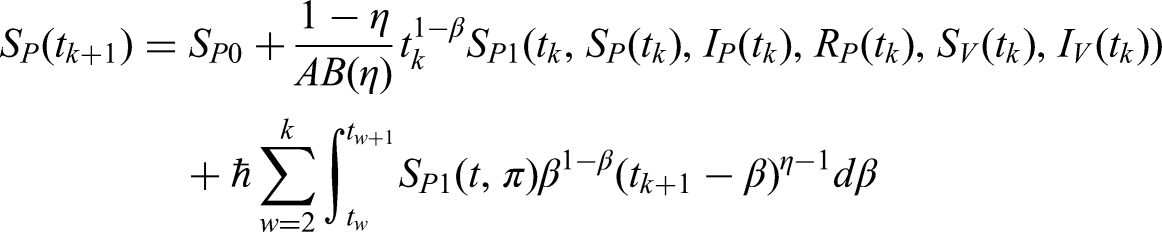
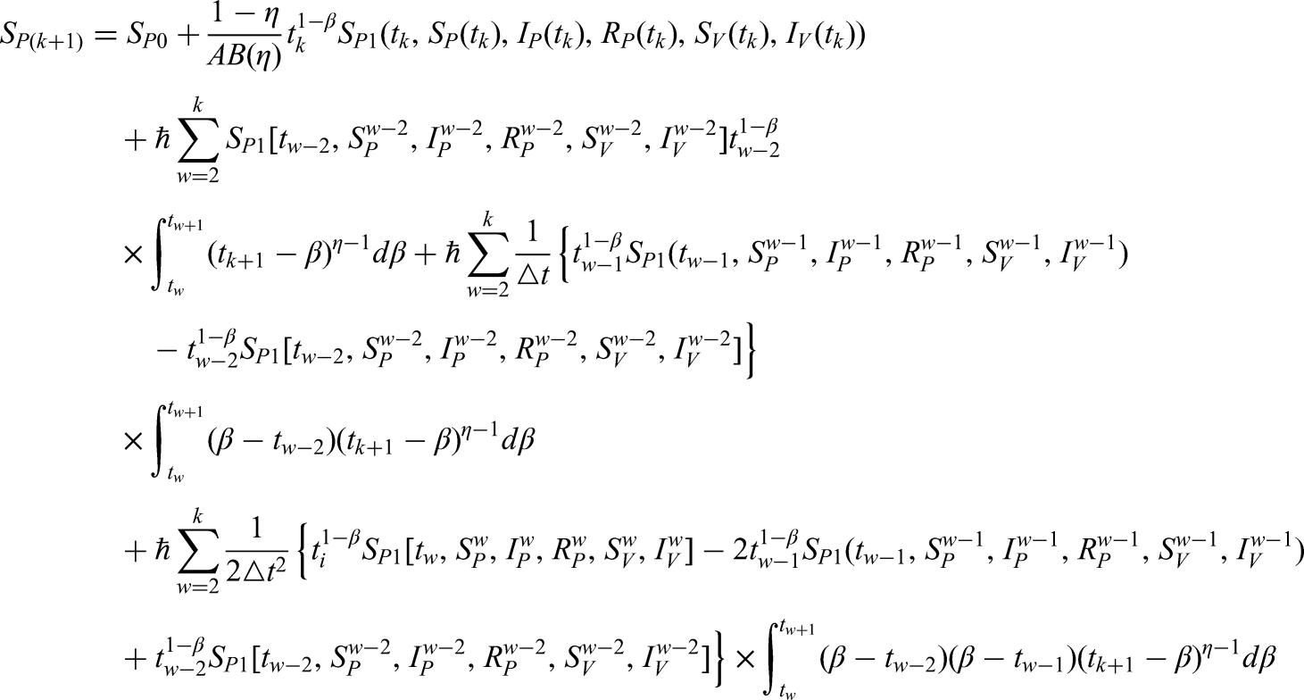
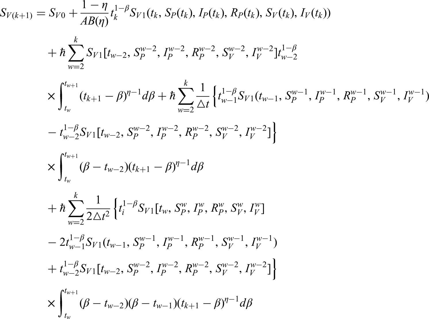
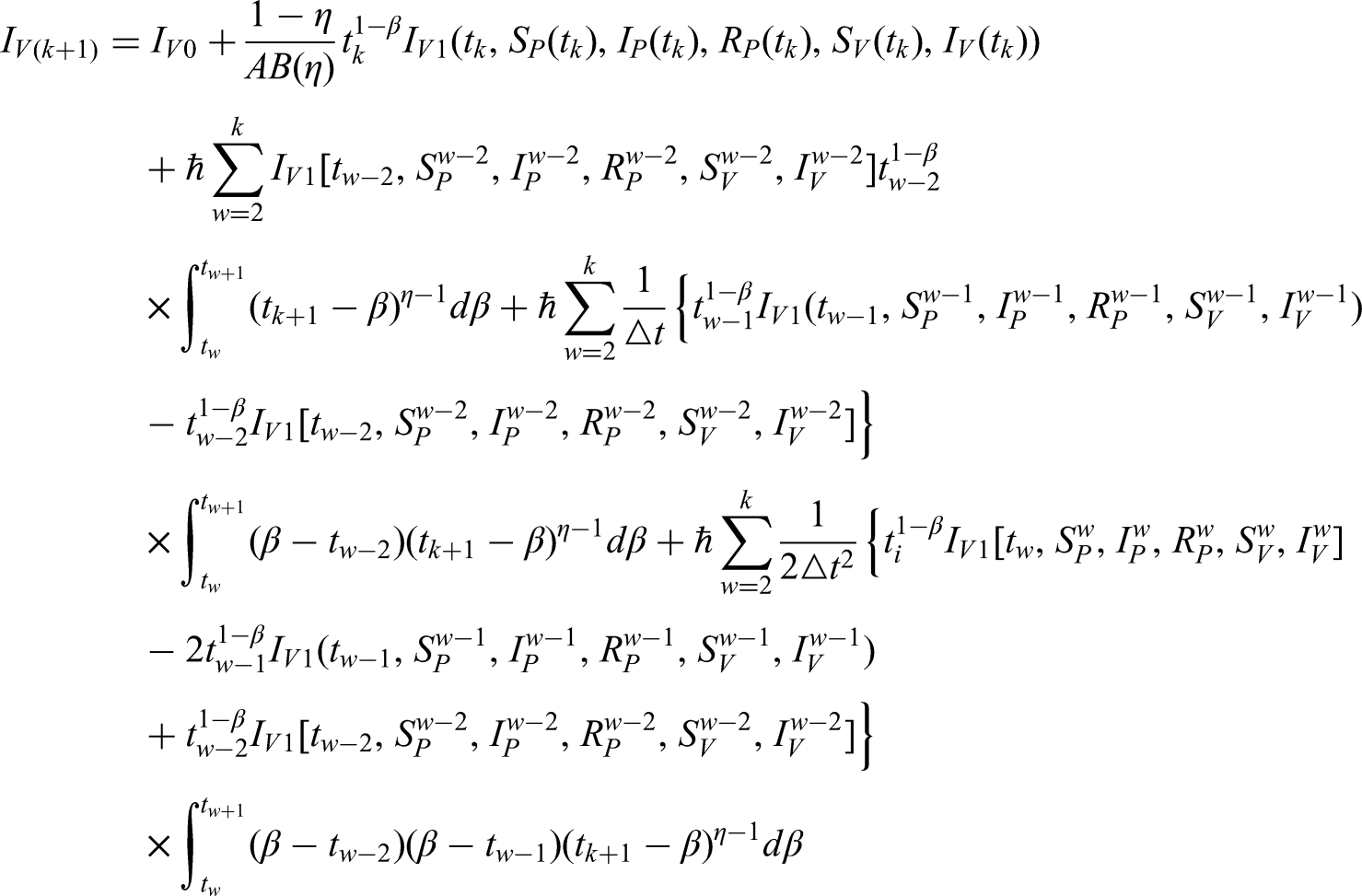
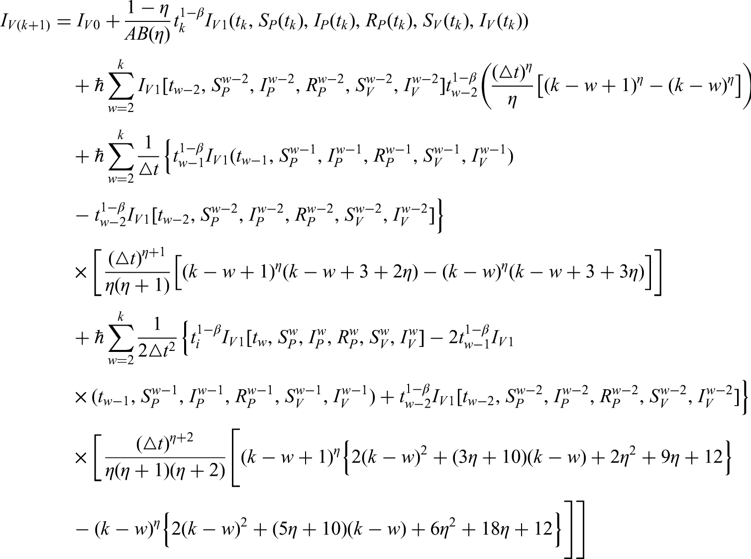
Solutions via the FFO

In this section, we employ a numerical approach to solve the newly formulated model given in equation (2). Specifically, the classical derivative operator is replaced by the ML kernel, while a variable-order version is also considered. For clarity, equation 2 can be rewritten in the following form:

$$\begin{array}{rl}{}_0^{FFM}{D}_t^{\eta ,\beta }{S}_P& ={\chi }_P-\delta S_P{I}_V+\varphi R_P-{\omega }_P{S}_P\\ {}_0^{FFM}{D}_t^{\eta ,\beta }{I}_P& =\delta S_P{I}_V-(\gamma +{ϵ}_P+{\omega }_P)I_P\\ {}_0^{FFM}{D}_t^{\eta ,\beta }{R}_P& =\gamma I_P-(\varphi +{\omega }_P)R_P\\ {}_0^{FFM}{D}_t^{\eta ,\beta }{S}_V& ={\chi }_V-\theta S_V{I}_P-{\omega }_V{S}_V\\ {}_0^{FFM}{D}_t^{\eta ,\beta }{I}_V& =\theta S_V{I}_P-({ϵ}_V+{\omega }_V)I_V\end{array}$$

The following results are obtained after using the FF integral and the ML kernel.

$$S_P(t_{k+1})=S_{P0}+\frac{1-\eta }{AB(\eta )}{t}_k^{1-\beta }{S}_{P1}(t_k,S_P(t_k),I_P(t_k),R_P(t_k),S_V(t_k),I_V(t_k))+\hslash \sum _{w=2}^k{\int }_{t_w}^{t_{w+1}}{S}_{P1}(t,\pi ){\beta }^{1-\beta }(t_{k+1}-\beta {)}^{\eta -1}d\beta$$

$$\begin{array}{rl}{I}_P(t_{\eta +1})& =I_{P0}+\frac{1-\eta }{AB(\eta )}{t}_k^{1-\beta }{I}_{P1}(t_k,S_P(t_k),I_P(t_k),R_P(t_k),S_V(t_k),I_V(t_k))\\ & +\hslash \sum _{w=2}^k{\int }_{t_w}^{t_{w+1}}{I}_{P1}(t,\pi ){\beta }^{1-\beta }(t_{k+1}-\beta {)}^{\eta -1}d\beta \\ R_P(t_{\eta +1})& =R_{P0}+\frac{1-\eta }{AB(\eta )}{t}_k^{1-\beta }{R}_{P1}(t_k,S_P(t_k),I_P(t_k),R_P(t_k),S_V(t_k),I_V(t_k))\\ & +\hslash \sum _{w=2}^k{\int }_{t_w}^{t_{w+1}}{R}_{P1}(t,\pi ){\beta }^{1-\beta }(t_{k+1}-\beta {)}^{\eta -1}d\beta \end{array}$$

$$\begin{array}{rl}{S}_V(t_{\eta +1})& =S_{V0}+\frac{1-\eta }{AB(\eta )}{t}_k^{1-\beta }{S}_{V1}(t_k,S_P(t_k),I_P(t_k),R_P(t_k),S_V(t_k),I_V(t_k))\\ & +\hslash \sum _{w=2}^k{\int }_{t_w}^{t_{w+1}}{S}_{V1}(t,\pi ){\beta }^{1-\beta }(t_{k+1}-\beta {)}^{\eta -1}d\beta \\ I_V(t_{\eta +1})& =I_{V0}+\frac{1-\eta }{AB(\eta )}{t}_k^{1-\beta }{I}_{V1}(t_k,S_P(t_k),I_P(t_k),R_P(t_k),S_V(t_k),I_V(t_k))\\ & +\hslash \sum _{w=2}^k{\int }_{t_w}^{t_{w+1}}{I}_{V1}(t,\pi ){\beta }^{1-\beta }(t_{k+1}-\beta {)}^{\eta -1}d\beta \end{array}$$

where $\pi =S_P,I_P,R_P,S_V,I_V$ and $\hslash =\frac{\eta }{AB(\eta )\mathrm{\Gamma }(\eta )}$ . Here, we recall the Newton polynomial:

$$\begin{array}{rl}\mathcal{A}(t,\pi )& \simeq \mathcal{A}(t_{k-2},S_{P(k-2)},P_{E(k-2)},I_{P(k-2)},R_{P(k-2)},S_{V(k-2)},I_{V(k-2)})\\ & +\frac{1}{\mathrm{△}t}\{\mathcal{A}(t_{k-1},S_{P(k-1)},P_{E(k-1)},I_{P(k-1)},R_{P(k-1)},S_{V(k-1)},I_{V(k-1)})\\ & -\mathcal{A}(t_{k-2},S_{P(k-2)},P_{E(k-2)},I_{P(k-2)},R_{P(k-2)},S_{V(k-2)},I_{V(k-2)})\}\times (\beta -t_{k-2})\\ & +\frac{1}{2\mathrm{△}{t}^2}\{\mathcal{A}(t,S_{Pk},P_{Ek},I_{Pk},R_{Pk},S_{Vk},I_{Vk})\\ & -2\mathcal{A}((t_{k-1},S_{P(k-1)},P_{E(k-1)},I_{P(k-1)},R_{P(k-1)},S_{V(k-1)},I_{V(k-1)}))\\ & -\mathcal{A}(t_{k-2},S_{P(k-2)},P_{E(k-2)},I_{P(k-2)},R_{P(k-2)},S_{V(k-2)},\\ & I_{V(k-2)})\}\times (\beta -t_{k-2})(\beta -t_{k-1})\end{array}$$

(17)

By replacing the Newton polynomial (17) in the previous equations, we get

$$\begin{array}{rl}{S}_{P(k+1)}& =S_{P0}+\frac{1-\eta }{AB(\eta )}{t}_k^{1-\beta }{S}_{P1}(t_k,S_P(t_k),I_P(t_k),R_P(t_k),S_V(t_k),I_V(t_k))\\ & +\hslash \sum _{w=2}^k{S}_{P1}[t_{w-2},S_P^{w-2},I_P^{w-2},R_P^{w-2},S_V^{w-2},I_V^{w-2}]t_{w-2}^{1-\beta }\\ & \times {\int }_{t_w}^{t_{w+1}}(t_{k+1}-\beta {)}^{\eta -1}d\beta +\hslash \sum _{w=2}^k\frac{1}{\mathrm{△}t}\{t_{w-1}^{1-\beta }{S}_{P1}(t_{w-1},S_P^{w-1},I_P^{w-1},R_P^{w-1},S_V^{w-1},I_V^{w-1})\\ & -t_{w-2}^{1-\beta }{S}_{P1}[t_{w-2},S_P^{w-2},I_P^{w-2},R_P^{w-2},S_V^{w-2},I_V^{w-2}]\}\\ & \times {\int }_{t_w}^{t_{w+1}}(\beta -t_{w-2})(t_{k+1}-\beta {)}^{\eta -1}d\beta \\ & +\hslash \sum _{w=2}^k\frac{1}{2\mathrm{△}{t}^2}\{t_i^{1-\beta }{S}_{P1}[t_w,S_P^w,I_P^w,R_P^w,S_V^w,I_V^w]-2t_{w-1}^{1-\beta }{S}_{P1}(t_{w-1},S_P^{w-1},I_P^{w-1},R_P^{w-1},S_V^{w-1},I_V^{w-1})\\ & +t_{w-2}^{1-\beta }{S}_{P1}[t_{w-2},S_P^{w-2},I_P^{w-2},R_P^{w-2},S_V^{w-2},I_V^{w-2}]\}\times {\int }_{t_w}^{t_{w+1}}(\beta -t_{w-2})(\beta -t_{w-1})(t_{k+1}-\beta {)}^{\eta -1}d\beta \end{array}$$

$$\begin{array}{rl}{I}_{P(k+1)}& =I_{P0}+\frac{1-\eta }{AB(\eta )}{t}_k^{1-\beta }{I}_{P1}(t_k,S_P(t_k),I_P(t_k),R_P(t_k),S_V(t_k),I_V(t_k))\\ & +\hslash \sum _{w=2}^k{I}_{P1}[t_{w-2},S_P^{w-2},I_P^{w-2},R_P^{w-2},S_V^{w-2},I_V^{w-2}]t_{w-2}^{1-\beta }\\ & \times {\int }_{t_w}^{t_{w+1}}(t_{k+1}-\beta {)}^{\eta -1}d\beta +\hslash \sum _{w=2}^k\frac{1}{\mathrm{△}t}\{t_{w-1}^{1-\beta }{I}_{P1}(t_{w-1},S_P^{w-1},I_P^{w-1},R_P^{w-1},S_V^{w-1},I_V^{w-1})\\ & -t_{w-2}^{1-\beta }{I}_{P1}[t_{w-2},S_P^{w-2},I_P^{w-2},R_P^{w-2},S_V^{w-2},I_V^{w-2}]\}\\ & \times {\int }_{t_w}^{t_{w+1}}(\beta -t_{w-2})(t_{k+1}-\beta {)}^{\eta -1}d\beta +\hslash \sum _{w=2}^k\frac{1}{2\mathrm{△}{t}^2}\{t_i^{1-\beta }\\ & I_{P1}[t_w,S_P^w,I_P^w,R_P^w,S_V^w,I_V^w]-2t_{w-1}^{1-\beta }{I}_{P1}(t_{w-1},S_P^{w-1},I_P^{w-1},R_P^{w-1},S_V^{w-1},I_V^{w-1})\\ & +t_{w-2}^{1-\beta }{I}_{P1}[t_{w-2},S_P^{w-2},I_P^{w-2},R_P^{w-2},S_V^{w-2},I_V^{w-2}]\}\\ & \times {\int }_{t_w}^{t_{w+1}}(\beta -t_{w-2})(\beta -t_{w-1})(t_{k+1}-\beta {)}^{\eta -1}d\beta \end{array}$$

$$\begin{array}{rl}{R}_{P(k+1)}& =R_{P0}+\frac{1-\eta }{AB(\eta )}{t}_k^{1-\beta }{R}_{P1}(t_k,S_P(t_k),I_P(t_k),R_P(t_k),S_V(t_k),I_V(t_k))\\ & +\hslash \sum _{w=2}^k{R}_{P1}[t_{w-2},S_P^{w-2},I_P^{w-2},R_P^{w-2},S_V^{w-2},I_V^{w-2}]t_{w-2}^{1-\beta }\\ & \times {\int }_{t_w}^{t_{w+1}}(t_{k+1}-\beta {)}^{\eta -1}d\beta +\hslash \sum _{w=2}^k\frac{1}{\mathrm{△}t}\{t_{w-1}^{1-\beta }{R}_{P1}(t_{w-1},S_P^{w-1},I_P^{w-1},R_P^{w-1},S_V^{w-1},I_V^{w-1})\\ & -t_{w-2}^{1-\beta }{R}_{P1}[t_{w-2},S_P^{w-2},I_P^{w-2},R_P^{w-2},S_V^{w-2},I_V^{w-2}]\}\\ & \times {\int }_{t_w}^{t_{w+1}}(\beta -t_{w-2})(t_{k+1}-\beta {)}^{\eta -1}d\beta +\hslash \sum _{w=2}^k\frac{1}{2\mathrm{△}{t}^2}\{t_i^{1-\beta }{R}_{P1}[t_w,S_P^w,I_P^w,R_P^w,S_V^w,I_V^w]\\ & -2t_{w-1}^{1-\beta }{R}_{P1}(t_{w-1},S_P^{w-1},I_P^{w-1},R_P^{w-1},S_V^{w-1},I_V^{w-1})\\ & +t_{w-2}^{1-\beta }{R}_{P1}[t_{w-2},S_P^{w-2},I_P^{w-2},R_P^{w-2},S_V^{w-2},I_V^{w-2}]\}\\ & \times {\int }_{t_w}^{t_{w+1}}(\beta -t_{w-2})(\beta -t_{w-1})(t_{k+1}-\beta {)}^{\eta -1}d\beta \end{array}$$

$$\begin{array}{rl}{S}_{V(k+1)}& =S_{V0}+\frac{1-\eta }{AB(\eta )}{t}_k^{1-\beta }{S}_{V1}(t_k,S_P(t_k),I_P(t_k),R_P(t_k),S_V(t_k),I_V(t_k))\\ & +\hslash \sum _{w=2}^k{S}_{V1}[t_{w-2},S_P^{w-2},I_P^{w-2},R_P^{w-2},S_V^{w-2},I_V^{w-2}]t_{w-2}^{1-\beta }\\ & \times {\int }_{t_w}^{t_{w+1}}(t_{k+1}-\beta {)}^{\eta -1}d\beta +\hslash \sum _{w=2}^k\frac{1}{\mathrm{△}t}\{t_{w-1}^{1-\beta }{S}_{V1}(t_{w-1},S_P^{w-1},I_P^{w-1},R_P^{w-1},S_V^{w-1},I_V^{w-1})\\ & -t_{w-2}^{1-\beta }{S}_{V1}[t_{w-2},S_P^{w-2},I_P^{w-2},R_P^{w-2},S_V^{w-2},I_V^{w-2}]\}\\ & \times {\int }_{t_w}^{t_{w+1}}(\beta -t_{w-2})(t_{k+1}-\beta {)}^{\eta -1}d\beta \\ & +\hslash \sum _{w=2}^k\frac{1}{2\mathrm{△}{t}^2}\{t_i^{1-\beta }{S}_{V1}[t_w,S_P^w,I_P^w,R_P^w,S_V^w,I_V^w]\\ & -2t_{w-1}^{1-\beta }{S}_{V1}(t_{w-1},S_P^{w-1},I_P^{w-1},R_P^{w-1},S_V^{w-1},I_V^{w-1})\\ & +t_{w-2}^{1-\beta }{S}_{V1}[t_{w-2},S_P^{w-2},I_P^{w-2},R_P^{w-2},S_V^{w-2},I_V^{w-2}]\}\\ & \times {\int }_{t_w}^{t_{w+1}}(\beta -t_{w-2})(\beta -t_{w-1})(t_{k+1}-\beta {)}^{\eta -1}d\beta \end{array}$$

$$\begin{array}{rl}{I}_{V(k+1)}& =I_{V0}+\frac{1-\eta }{AB(\eta )}{t}_k^{1-\beta }{I}_{V1}(t_k,S_P(t_k),I_P(t_k),R_P(t_k),S_V(t_k),I_V(t_k))\\ & +\hslash \sum _{w=2}^k{I}_{V1}[t_{w-2},S_P^{w-2},I_P^{w-2},R_P^{w-2},S_V^{w-2},I_V^{w-2}]t_{w-2}^{1-\beta }\\ & \times {\int }_{t_w}^{t_{w+1}}(t_{k+1}-\beta {)}^{\eta -1}d\beta +\hslash \sum _{w=2}^k\frac{1}{\mathrm{△}t}\{t_{w-1}^{1-\beta }{I}_{V1}(t_{w-1},S_P^{w-1},I_P^{w-1},R_P^{w-1},S_V^{w-1},I_V^{w-1})\\ & -t_{w-2}^{1-\beta }{I}_{V1}[t_{w-2},S_P^{w-2},I_P^{w-2},R_P^{w-2},S_V^{w-2},I_V^{w-2}]\}\\ & \times {\int }_{t_w}^{t_{w+1}}(\beta -t_{w-2})(t_{k+1}-\beta {)}^{\eta -1}d\beta +\hslash \sum _{w=2}^k\frac{1}{2\mathrm{△}{t}^2}\{t_i^{1-\beta }{I}_{V1}[t_w,S_P^w,I_P^w,R_P^w,S_V^w,I_V^w]\\ & -2t_{w-1}^{1-\beta }{I}_{V1}(t_{w-1},S_P^{w-1},I_P^{w-1},R_P^{w-1},S_V^{w-1},I_V^{w-1})\\ & +t_{w-2}^{1-\beta }{I}_{V1}[t_{w-2},S_P^{w-2},I_P^{w-2},R_P^{w-2},S_V^{w-2},I_V^{w-2}]\}\\ & \times {\int }_{t_w}^{t_{w+1}}(\beta -t_{w-2})(\beta -t_{w-1})(t_{k+1}-\beta {)}^{\eta -1}d\beta \end{array}$$

The following techniques can be used to calculate the integral in the equations that were previously discussed.

$$\begin{array}{cc}& {\int }_{t_w}^{t_{w+1}}(t_{k+1}-\beta {)}^{\eta -1}d\beta =\frac{(\mathrm{△}t{)}^{\eta }}{\eta }[(k-w+1{)}^{\eta }-(k-w{)}^{\eta }]\\ & \begin{array}{rl}{\int }_{t_w}^{t_{w+1}}(\beta -t_{w-2})(t_{k+1}-\beta {)}^{\eta -1}d\beta & =\frac{(\mathrm{△}t{)}^{\eta +1}}{\eta (\eta +1)}[(k-w+1{)}^{\eta }(k-w+3+2\eta )\\ & -(k-w{)}^{\eta }(k-w+3+3\eta )]\end{array}\\ & \begin{array}{rl}& {\int }_{t_w}^{t_{w+1}}(\beta -t_{w-2})(\beta -t_{w-1})(t_{k+1}-\beta {)}^{\eta -1}d\beta \\ & =\frac{(\mathrm{△}t{)}^{\eta +2}}{\eta (\eta +1)(\eta +2)}[(k-w+1{)}^{\eta }\{2(k-w{)}^2+(3\eta +10)(k-w)+2{\eta }^2\end{array}\\ & +9\eta +12\}-(k-w{)}^{\eta }\{2(k-w{)}^2+(5\eta +10)(k-w)+6{\eta }^2+18\eta +12\}]\end{array}$$

Hence, we get finally

$$\begin{array}{rl}{S}_{P(k+1)}& =S_{P0}+\frac{1-\eta }{AB(\eta )}{t}_k^{1-\beta }{S}_{P1}(t_k,S_P(t_k),I_P(t_k),R_P(t_k),S_V(t_k),I_V(t_k))\\ & +\hslash \sum _{w=2}^k{S}_{P1}[t_{w-2},S_P^{w-2},I_P^{w-2},R_P^{w-2},S_V^{w-2},\\ & I_V^{w-2}]t_{w-2}^{1-\beta }\times \left(\frac{(\mathrm{△}t{)}^{\eta }}{\eta }[(k-w+1{)}^{\eta }-(k-w{)}^{\eta }]\right)\\ & +\hslash \sum _{w=2}^k\frac{1}{\mathrm{△}t}\{t_{w-1}^{1-\beta }{S}_{P1}(t_{w-1},S_P^{w-1},I_P^{w-1},R_P^{w-1},S_V^{w-1},I_V^{w-1})\\ & -t_{w-2}^{1-\beta }{S}_{P1}[t_{w-2},S_P^{w-2},I_P^{w-2},R_P^{w-2},S_V^{w-2},I_V^{w-2}]\}\\ & \times [\frac{(\mathrm{△}t{)}^{\eta +1}}{\eta (\eta +1)}[(k-w+1{)}^{\eta }(k-w+3+2\eta )-(k-w{)}^{\eta }(k-w+3+3\eta )]]\\ & +\hslash \sum _{w=2}^k\frac{1}{2\mathrm{△}{t}^2}\{t_i^{1-\beta }{S}_{P1}[t_w,S_P^w,I_P^w,R_P^w,S_V^w,I_V^w]-2t_{w-1}^{1-\beta }{S}_{P1}(t_{w-1},S_P^{w-1},I_P^{w-1},R_P^{w-1},\\ & S_V^{w-1},I_V^{w-1})+t_{w-2}^{1-\beta }{S}_{P1}[t_{w-2},S_P^{w-2},I_P^{w-2},R_P^{w-2},S_V^{w-2},I_V^{w-2}]\}\\ & \times [\frac{(\mathrm{△}t{)}^{\eta +2}}{\eta (\eta +1)(\eta +2)}[(k-w+1{)}^{\eta }\{2(k-w{)}^2+(3\eta +10)(k-w)+2{\eta }^2+9\eta +12\}\\ & -(k-w{)}^{\eta }\{2(k-w{)}^2+(5\eta +10)(k-w)+6{\eta }^2+18\eta +12\}]]\end{array}$$

$$\begin{array}{rl}{I}_{P(k+1)}& =I_{P0}+\frac{1-\eta }{AB(\eta )}{t}_k^{1-\beta }{I}_{P1}(t_k,S_P(t_k),I_P(t_k),R_P(t_k),S_V(t_k),I_V(t_k))\\ & +\hslash \sum _{w=2}^k{I}_{P1}[t_{w-2},S_P^{w-2},I_P^{w-2},R_P^{w-2},S_V^{w-2},I_V^{w-2}]t_{w-2}^{1-\beta }\left(\frac{(\mathrm{△}t{)}^{\eta }}{\eta }[(k-w+1{)}^{\eta }-(k-w{)}^{\eta }]\right)\\ & +\hslash \sum _{w=2}^k\frac{1}{\mathrm{△}t}\{t_{w-1}^{1-\beta }{I}_{P1}(t_{w-1},S_P^{w-1},I_P^{w-1},R_P^{w-1},S_V^{w-1},I_V^{w-1})\\ & -t_{w-2}^{1-\beta }{I}_{P1}[t_{w-2},S_P^{w-2},I_P^{w-2},R_P^{w-2},S_V^{w-2},I_V^{w-2}]\}\\ & \times [\frac{(\mathrm{△}t{)}^{\eta +1}}{\eta (\eta +1)}[(k-w+1{)}^{\eta }(k-w+3+2\eta )-(k-w{)}^{\eta }(k-w+3+3\eta )]]\\ & +\hslash \sum _{w=2}^k\frac{1}{2\mathrm{△}{t}^2}\{t_i^{1-\beta }{I}_{P1}[t_w,S_P^w,I_P^w,R_P^w,S_V^w,I_V^w]-2t_{w-1}^{1-\beta }{I}_{P1}(t_{w-1},S_P^{w-1},I_P^{w-1},R_P^{w-1},\\ & \times S_V^{w-1},I_V^{w-1})+t_{w-2}^{1-\beta }{I}_{P1}[t_{w-2},S_P^{w-2},I_P^{w-2},R_P^{w-2},S_V^{w-2},I_V^{w-2}]\}\\ & \times [\frac{(\mathrm{△}t{)}^{\eta +2}}{\eta (\eta +1)(\eta +2)}[(k-w+1{)}^{\eta }\{2(k-w{)}^2+(3\eta +10)(k-w)+2{\eta }^2+9\eta +12\}\\ & -(k-w{)}^{\eta }\{2(k-w{)}^2+(5\eta +10)(k-w)+6{\eta }^2+18\eta +12\}]]\end{array}$$

$$\begin{array}{rl}{R}_{P(k+1)}& =R_{P0}+\frac{1-\eta }{AB(\eta )}{t}_k^{1-\beta }{R}_{P1}(t_k,S_P(t_k),I_P(t_k),R_P(t_k),S_V(t_k),I_V(t_k))\\ & +\hslash \sum _{w=2}^k{R}_{P1}[t_{w-2},S_P^{w-2},I_P^{w-2},R_P^{w-2},S_V^{w-2},I_V^{w-2}]t_{w-2}^{1-\beta }\times \left(\frac{(\mathrm{△}t{)}^{\eta }}{\eta }[(k-w+1{)}^{\eta }-(k-w{)}^{\eta }]\right)\\ & +\hslash \sum _{w=2}^k\frac{1}{\mathrm{△}t}\{t_{w-1}^{1-\beta }{R}_{P1}(t_{w-1},S_P^{w-1},I_P^{w-1},R_P^{w-1},S_V^{w-1},I_V^{w-1})\\ & -t_{w-2}^{1-\beta }{R}_{P1}[t_{w-2},S_P^{w-2},I_P^{w-2},R_P^{w-2},S_V^{w-2},I_V^{w-2}]\}\\ & \times [\frac{(\mathrm{△}t{)}^{\eta +1}}{\eta (\eta +1)}[(k-w+1{)}^{\eta }(k-w+3+2\eta )-(k-w{)}^{\eta }(k-w+3+3\eta )]]\\ & +\hslash \sum _{w=2}^k\frac{1}{2\mathrm{△}{t}^2}\{t_i^{1-\beta }{R}_{P1}[t_w,S_P^w,I_P^w,R_P^w,S_V^w,I_V^w]-2t_{w-1}^{1-\beta }{R}_{P1}(t_{w-1},S_P^{w-1},I_P^{w-1},R_P^{w-1},\\ & \times S_V^{w-1},I_V^{w-1})+t_{w-2}^{1-\beta }{R}_{P1}[t_{w-2},S_P^{w-2},I_P^{w-2},R_P^{w-2},S_V^{w-2},I_V^{w-2}]\}\\ & \times [\frac{(\mathrm{△}t{)}^{\eta +2}}{\eta (\eta +1)(\eta +2)}[(k-w+1{)}^{\eta }\{2(k-w{)}^2+(3\eta +10)(k-w)+2{\eta }^2+9\eta +12\}\\ & -(k-w{)}^{\eta }\{2(k-w{)}^2+(5\eta +10)(k-w)+6{\eta }^2+18\eta +12\}]]\end{array}$$

$$\begin{array}{rl}{S}_{V(k+1)}& =S_{V0}+\frac{1-\eta }{AB(\eta )}{t}_k^{1-\beta }{S}_{V1}(t_k,S_P(t_k),I_P(t_k),R_P(t_k),S_V(t_k),I_V(t_k))\\ & +\hslash \sum _{w=2}^k{S}_{V1}[t_{w-2},S_P^{w-2},I_P^{w-2},R_P^{w-2},S_V^{w-2},I_V^{w-2}]t_{w-2}^{1-\beta }\left(\frac{(\mathrm{△}t{)}^{\eta }}{\eta }[(k-w+1{)}^{\eta }-(k-w{)}^{\eta }]\right)\\ & +\hslash \sum _{w=2}^k\frac{1}{\mathrm{△}t}\{t_{w-1}^{1-\beta }{S}_{V1}(t_{w-1},S_P^{w-1},I_P^{w-1},R_P^{w-1},S_V^{w-1},I_V^{w-1})\\ & -t_{w-2}^{1-\beta }{S}_{V1}[t_{w-2},S_P^{w-2},I_P^{w-2},R_P^{w-2},S_V^{w-2},I_V^{w-2}]\}\\ & \times [\frac{(\mathrm{△}t{)}^{\eta +1}}{\eta (\eta +1)}[(k-w+1{)}^{\eta }(k-w+3+2\eta )-(k-w{)}^{\eta }(k-w+3+3\eta )]]\\ & +\hslash \sum _{w=2}^k\frac{1}{2\mathrm{△}{t}^2}\{t_i^{1-\beta }{S}_{V1}[t_w,S_P^w,I_P^w,R_P^w,S_V^w,I_V^w]-2t_{w-1}^{1-\beta }{S}_{V1}(t_{w-1},S_P^{w-1},I_P^{w-1},R_P^{w-1},\\ & \times S_V^{w-1},I_V^{w-1})+t_{w-2}^{1-\beta }{S}_{V1}[t_{w-2},S_P^{w-2},I_P^{w-2},R_P^{w-2},S_V^{w-2},I_V^{w-2}]\}\\ & \times [\frac{(\mathrm{△}t{)}^{\eta +2}}{\eta (\eta +1)(\eta +2)}[(k-w+1{)}^{\eta }\{2(k-w{)}^2+(3\eta +10)(k-w)+2{\eta }^2+9\eta +12\}\\ & -(k-w{)}^{\eta }\{2(k-w{)}^2+(5\eta +10)(k-w)+6{\eta }^2+18\eta +12\}]]\end{array}$$

$$\begin{array}{rl}{I}_{V(k+1)}& =I_{V0}+\frac{1-\eta }{AB(\eta )}{t}_k^{1-\beta }{I}_{V1}(t_k,S_P(t_k),I_P(t_k),R_P(t_k),S_V(t_k),I_V(t_k))\\ & +\hslash \sum _{w=2}^k{I}_{V1}[t_{w-2},S_P^{w-2},I_P^{w-2},R_P^{w-2},S_V^{w-2},I_V^{w-2}]t_{w-2}^{1-\beta }\left(\frac{(\mathrm{△}t{)}^{\eta }}{\eta }[(k-w+1{)}^{\eta }-(k-w{)}^{\eta }]\right)\\ & +\hslash \sum _{w=2}^k\frac{1}{\mathrm{△}t}\{t_{w-1}^{1-\beta }{I}_{V1}(t_{w-1},S_P^{w-1},I_P^{w-1},R_P^{w-1},S_V^{w-1},I_V^{w-1})\\ & -t_{w-2}^{1-\beta }{I}_{V1}[t_{w-2},S_P^{w-2},I_P^{w-2},R_P^{w-2},S_V^{w-2},I_V^{w-2}]\}\\ & \times [\frac{(\mathrm{△}t{)}^{\eta +1}}{\eta (\eta +1)}[(k-w+1{)}^{\eta }(k-w+3+2\eta )-(k-w{)}^{\eta }(k-w+3+3\eta )]]\\ & +\hslash \sum _{w=2}^k\frac{1}{2\mathrm{△}{t}^2}\{t_i^{1-\beta }{I}_{V1}[t_w,S_P^w,I_P^w,R_P^w,S_V^w,I_V^w]-2t_{w-1}^{1-\beta }{I}_{V1}\\ & \times (t_{w-1},S_P^{w-1},I_P^{w-1},R_P^{w-1},S_V^{w-1},I_V^{w-1})+t_{w-2}^{1-\beta }{I}_{V1}[t_{w-2},S_P^{w-2},I_P^{w-2},R_P^{w-2},S_V^{w-2},I_V^{w-2}]\}\\ & \times [\frac{(\mathrm{△}t{)}^{\eta +2}}{\eta (\eta +1)(\eta +2)}[(k-w+1{)}^{\eta }\{2(k-w{)}^2+(3\eta +10)(k-w)+2{\eta }^2+9\eta +12\}\\ & -(k-w{)}^{\eta }\{2(k-w{)}^2+(5\eta +10)(k-w)+6{\eta }^2+18\eta +12\}]]\end{array}$$

Simulation explanation

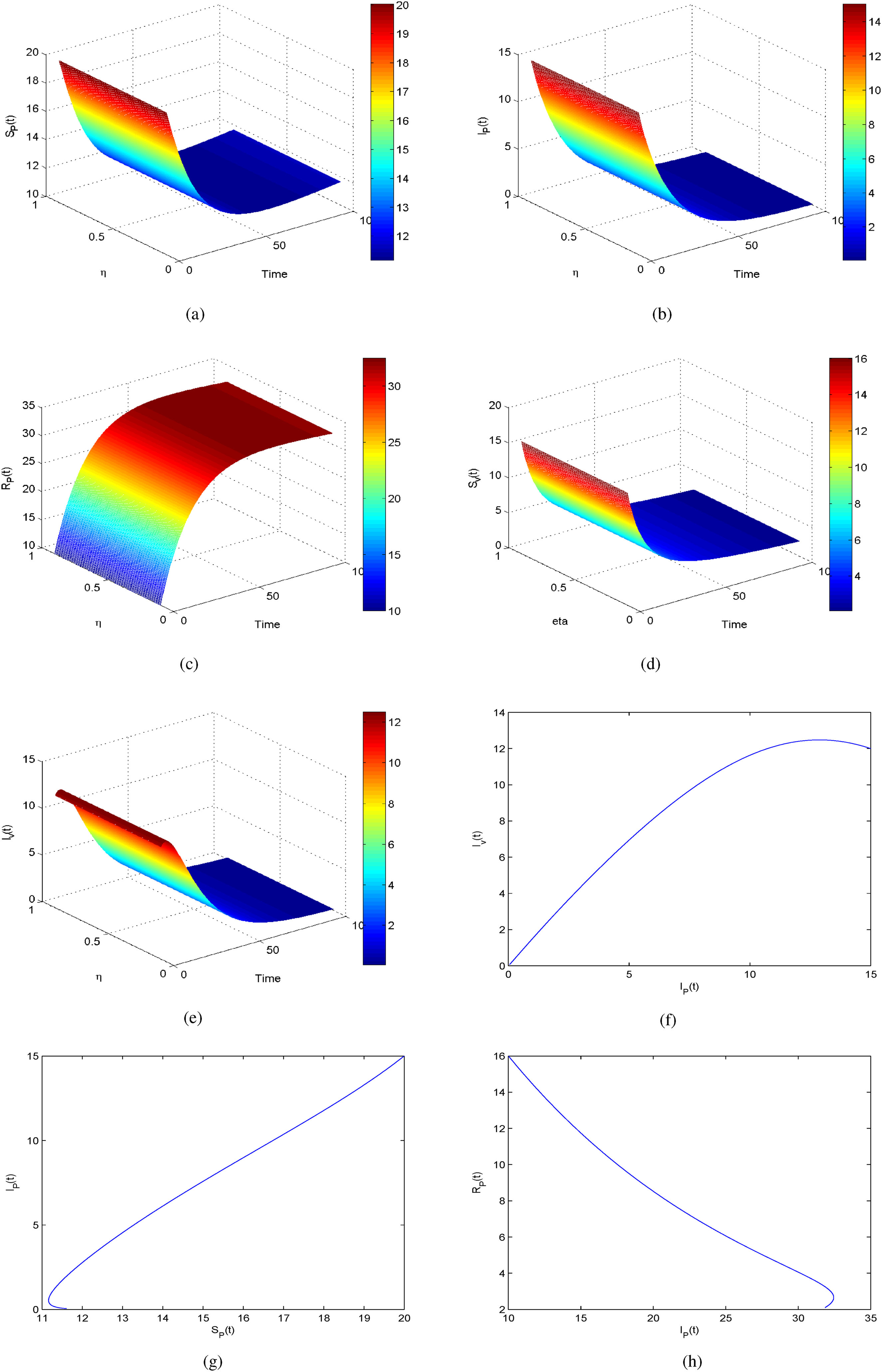
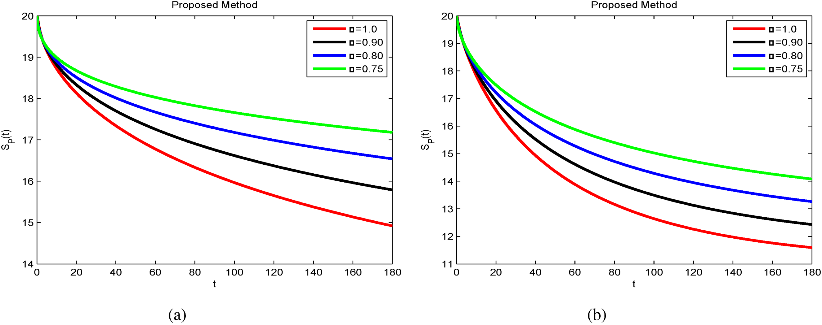
This section presents numerical simulations to validate the theoretical results obtained for the anthracnose disease model. By incorporating non-integer parameter values, significant and insightful outcomes are achieved. As the fractional order decreases, the solutions for $S_P$ , $I_P$ , $R_P$ , $S_V$ , and $I_V$ (see Figures 7 to 11) converge towards the desired behavior. The simulations were performed in MATLAB, with initial conditions set as $S_P(0)=20$ , $I_P(0)=15$ , $R_P(0)=10$ , $S_V(0)=16$ , and $I_V(0)=12$ across the corresponding sub-compartments.

Figure 7.

Numerical simulation of the $S_P(t)$ compartment of the system under varying fractal dimension $\beta$ and fractional order $\eta$ . (a) $\beta =0.6$ and (b) $\beta =0.4$ .

Figure 8.

Numerical simulation of the $I_P(t)$ compartment of the system under varying fractal dimension $\beta$ and fractional order $\eta$ . (a) $\beta =0.6$ and (b) $\beta =0.4$ .

Figure 9.

Numerical simulation of the $R_P(t)$ compartment of the system under varying fractal dimension $\beta$ and fractional order $\eta$ . (a) $\beta =0.6$ and (b) $\beta =0.4$ .

Figure 10.

Numerical simulation of the $S_V(t)$ compartment of the system under varying fractal dimension $\beta$ and fractional order $\eta$ . (a) $\beta =0.6$ and (b) $\beta =0.4$ .

Figure 11.

Numerical simulation of the $I_V(t)$ compartment of the system under varying fractal dimension $\beta$ and fractional order $\eta$ . (a) $\beta =0.6$ and (b) $\beta =0.4$ .

The simulation outcomes of the proposed anthracnose model, obtained under both integer-order operator and FFO, are illustrated in Figures 7 to 11. Each figure highlights the dynamic behavior of specific compartments influenced by splashing-rain transmission and hypersensitive response mechanisms.

Figure 7 presents the temporal evolution of susceptible plants ( $S_P$ ). The population of healthy plants declines gradually as infection spreads, before stabilizing at a lower steady state. This indicates that the disease pressure reduces the pool of susceptible plants until recovery mechanisms dominate.

Figure 8 depicts the infected plant compartment ( $I_P$ ). Initially, infection levels rise sharply due to exposure to infected vectors, but then decline as recovery and hypersensitive response effects counteract disease progression. The fractional-order curves demonstrate slower decay compared to the integer-order case, highlighting the influence of memory effects on prolonged infection persistence.

Figure 9 shows the recovered plant population ( $R_P$ ), which increases monotonically over time and eventually stabilizes at equilibrium. The higher recovery rate under fractional dynamics suggests enhanced disease control when memory-dependent processes are considered.

Figure 10 illustrates the susceptible vector class ( $S_V$ ). A decreasing trend is observed as vectors acquire infection through contact with infected plants. The fractional model reveals smoother transitions and delayed stabilization, implying environmental feedback in vector behavior.

Figure 11 represents the infected vector population ( $I_V$ ). The infected vectors diminish progressively, signifying the eventual containment of the disease through natural death and reduced plant infection sources. The slower convergence in the fractional model captures the long-term influence of environmental persistence on vector infection.

Overall, the fractional-order results depict smoother, delayed responses across compartments, reflecting the realistic biological memory effects in anthracnose dynamics. These findings emphasize that incorporating FFOs provides a more accurate description of infection decay and recovery behavior compared to the classical integer-order model.

Furthermore, Figures 7(a) to 11(a) and 7(b) to 11(b) confirm that while the overall behaviors remain similar, reducing the fractional order from $0.6$ to $0.4$ produces more accurate and reliable results. Notably, Figure 9(a) and (b) indicates that the recovered population grows significantly when fractional values decrease, reflecting the effectiveness of early stage fungicide treatment and continuous monitoring. These findings highlight the predictive capability of the model in reducing the prevalence of infected plants and vectors in the environment. Compared with the classical derivative approach, the FFO produces more precise and stable solutions across all sub-compartments. The results further suggest that lowering the fractional order enhances the accuracy and reliability of the model predictions.

Conclusion

In this work, we proposed a nonlinear compartmental model to describe the transmission dynamics of anthracnose disease in plants caused by splashing-rain. The model incorporates the FFO to obtain reliable results and better capture environmental interactions. Our analysis highlights that recovery without external medical intervention can significantly reduce the prevalence of infection, thereby facilitating early elimination of the disease from the environment. Both qualitative and numerical investigations confirm the stability, boundedness, and uniqueness of solutions for the proposed fractional-order system. Simulation results verify that the anthracnose disease persists under certain conditions but can be effectively reduced through appropriate control measures such as cutting and burying infected plants. The model also demonstrates that bifurcation does not occur under different parameter variations, and chaos control ensures that the system remains within a bounded domain. The influence of the fractional operator is further explored using numerical simulations based on Lagrange polynomial approximations. These results reveal how fractional dynamics provide a more accurate representation of nonlocal interactions and HRs, thereby strengthening plant resistance against pathogen spread through splashing rain. Overall, the proposed model enhances understanding of anthracnose dynamics by improving long-term forecasts and offering practical strategies for disease management. The findings emphasize the role of fractional modeling in predicting the behavior of plant diseases and contribute valuable insights for future research and effective control strategies aimed at reducing the impact of anthracnose in agricultural environments. The developed model provides a predictive tool to determine optimal fungicide application timing under varying rainfall conditions. It can assist farmers and agricultural managers in implementing timely interventions to minimize anthracnose spread and improve crop resilience. Future research can address these limitations by integrating climate-dependent and spatially explicit parameters to capture environmental variability more accurately. The inclusion of stochastic components or delay terms could also enhance model realism by accounting for unpredictable weather fluctuations and latent infection periods. Additionally, parameter estimation based on experimental or field surveillance data would improve model calibration and predictive reliability. Finally, coupling the present model with optimal control theory could guide the timing and dosage of fungicide applications, providing practical recommendations for sustainable disease management under varying rainfall conditions.