A method for calculating differential constitutive equation of linear viscoelastic composite model

Abstract

The stress–strain behaviors of viscoelastic materials are often simulated using a model composed of various combinations of springs and dampers. With the increase in the number of springs and dampers, the viscoelastic characteristics of the model will approach those of the actual material. This study discusses how to obtain the differential constitutive equation of a viscoelastic model composed of any number of springs and dampers. First, the general viscoelastic model is regarded as the combination of various Kelvin units. The viscoelastic model is then transformed into a digraph. Based on the relationships between the independent path of the digraph and the strain equation of the viscoelastic model and between the closed enclosure and the stress equation, the derivation of the constitutive equation is transformed into operations involving the incidence matrix of the digraph. Finally, the coefficients of the linear differential operator of the constitutive equation of the viscoelastic model can be obtained by block matrix operations. This method is suitable for computer programming and has a certain significance for accurately constructing viscoelastic models of engineering materials.

Introduction

Viscoelastic materials are widely used in various applications. These materials include industrial materials, such as plastics and rubber, geological materials, such as soil and asphalt, and biological materials, such as muscle and blood. Materials with viscoelastic properties are too numerous to enumerate. Because viscoelastic materials have both elastic and viscous properties, their mechanical properties depend on the environmental temperature and the loading time, rate, and amplitude. It is very important for engineering applications and theoretical research to establish a suitable model to accurately describe the viscoelastic behaviors of materials. The description of the viscoelastic properties and the expressions of the constitutive equations of materials are also important subjects of viscoelastic theory.

To simulate the stress–strain behaviors of viscoelastic materials, models composed of springs, dashpots, and their various combinations are often used. Examples of such models include the Maxwell model, Kelvin model, Poynting–Thomson model, Burgers model, generalized Maxwell model, and generalized Kelvin model. Over the years, a variety of models have been developed to characterize the viscoelastic properties of materials, and many studies have been carried to determine mathematical descriptions of the constitutive equations of viscoelastic materials. ¹ Using these models, many scholars have conducted extensive research in various engineering fields. For example, Ren et al. ² used the improved Burgers model to explore the vibration characteristics of viscoelastic composite structures. Huang et al. ³ also used the modified Burgers model to describe the viscoelastic constitutive behavior of asphalt concrete. Xu et al. ⁴ modeled the viscoelastic behaviors of asphalt binders and asphalt mastics using the FDM-4 model, which was composed of a Maxwell element in series with two Abel dashpots. Baglieri et al. ⁵ studied the viscoelastic characteristics of a set of polymer-modified bituminous binders based on a three-parameter viscoelastic model that consisted of a dashpot in series with a springpot. Nguyen et al. ⁶ investigated the effective viscoelastic properties of materials containing micro-cracks with random orientations and parallel distributions using the generalized Maxwell model. The various models have different advantages and disadvantages. For example, the Maxwell model can simulate the phenomenon of stress relaxation but cannot represent the creep process. The Kelvin model can simulate creep but cannot represent stress relaxation.^7,8 In general, with the increase in the number of springs and dampers, the viscoelastic characteristics that the model can simulate approach those of the actual material. ⁹ However, for the viscoelastic model composed of any number of springs and dampers linked in any way, determining how to derive the differential constitutive equation is not shown in various viscoelastic theory textbooks. Compared with classical viscoelastic models, the fractional viscoelastic models have also been studied by many researchers. Su et al. ¹⁰ established the generalized fractional models with the Laplace transform method. A number of scholars continue to study the Laplace transform or extend its application scenario. ¹¹ Regardless of whether it is a linear viscoelasticity model or a fractional viscoelastic model, the Laplace transform is a very good method.

In this study, the differential constitutive equation of the Poynting–Thomson model is taken as an example. Based on the corresponding relation between the viscoelastic model and digraph, the general form of the differential constitutive equation of an arbitrary viscoelastic composite model expressed in matrix form is derived. The stress–strain differential equations of a more complex model composed of 10 springs and dampers are quickly solved using this algorithm. This method is suitable for computer programming and has significance for accurately constructing the viscoelastic models of practical materials and accurately describing the viscoelastic characteristics and stress–strain behaviors of engineering materials.

Matrix form of constitutive equation of Poynting–Thomson model

The differential constitutive equation of the Poynting–Thomson model is given in textbooks on viscoelastic theory,^8,9 but the derivation process is not given. Of course, owing to the small number of springs and dampers, the derivation process is not difficult. Below, the general form of differential constitutive equation of an arbitrary viscoelastic model is summarized and established by formulating the differential constitutive equation of the Poynting–Thomson model in matrix form.

As shown in Figure 1, the stress–strain law of a Kelvin basic unit is as follows:

$$\sigma =E\epsilon +\eta \frac{d\epsilon }{\mathrm{dt}}$$

(1)

Figure 1.

Kelvin unit.

To ensure that the method can be applied to any linear viscoelastic composite model, the general viscoelastic model is regarded as a combination of various Kelvin units. When there is a separate spring or damper in the viscoelastic model that cannot form the Kelvin unit, a spring with an elastic parameter of 0 or a damper with the viscous parameter of 0 can be added. For example, the Poynting–Thomson model shown in Figure 2 can be extended to a model composed of Kelvin units by adding a corresponding spring and damper, as shown in Figure 3(a), and then all the non-Kelvin units in the model are extended to Kelvin units, as shown in Figure 3(b). First, the differential constitutive equation of the viscoelastic model shown in Figure 3 is formulated, and η₁, η₂, and E₃ are set to 0, which is equivalent to the original Poynting–Thomson model shown in Figure 2. Each Kelvin unit is transformed into a directed edge, and then a directed graph can be formed. Figure 4 shows the digraph G₁ = (V, E) corresponding to the Poynting–Thomson model.

Figure 2.

Poynting–Thomson model.

Figure 3.

(a) The standard form of the Poynting–Thomson model and (b) corresponding to the Kelvin unit model.

Figure 4.

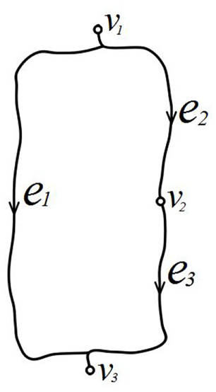
Digraph corresponding to the Poynting–Thomson model.

Let the total strain of the Poynting–Thomson model in Figure 3 be ε, and the strains of Kelvin unit 1, Kelvin unit 2, and Kelvin unit 3 be ε₁, ε₂, and ε₃ respectively. The relationship between the total strain ε of the model and the strain ε _i of each Kelvin unit can be determined based on the route from the starting point to the end point in the digraph. There is a corresponding relationship between them. The extended standard model of the Poynting–Thomson model shown in Figure 3 has two equations for the total strain ε and the strain ε _i of each Kelvin unit, namely,

$$\epsilon ={\epsilon }_1$$

(2)

$$\epsilon ={\epsilon }_2+{\epsilon }_3$$

(3)

In the digraph corresponding to the Poynting–Thomson model shown in Figure 4, there are two independent routes from the starting point to the end point. They are as follows: route (1) starting point → e₁ → end point; route (2) starting point → e₂ → e₃ → end point, as shown in Figure 5.

Figure 5.

Routes of digraph G₁ = (V, E).

The incidence matrix of the digraph G₁ = (V, E) shown in Figure 4 is as follows:

$$M=\begin{array}{cc}\multicolumn{1}{c}{\left[\begin{array}{ccc}{e}_1\hfill & e_2\hfill & e_3\hfill \\ 1\hfill & 1\hfill & 0\hfill \\ \multicolumn{1}{c}{0}& -1\hfill & 1\hfill \\ \multicolumn{1}{c}{-1}& 0\hfill & -1\hfill \end{array}\right]}& \begin{array}{c}{v}_1\hfill \\ \multicolumn{1}{c}{v_2}\\ \multicolumn{1}{c}{v_3}\end{array}\hfill \end{array}$$

(4)

Each column of the above matrix, M, corresponds to a directed edge of the digraph G₁ = (V, E), with each row corresponding to all of the vertices. If vertex v_i is the head of the edge e_j, then the ith row and the jth column of matrix M is 1. If vertex v_i is the tail of the edge, e_j, then the ith row and the jth column of matrix M is −1. Except for these two cases, everything else is 0.

Solution for x of the route matrix of a digraph is the linearly independent solutions of the following equation (when the element of x can only be 1 or 0):

$$M·x=\begin{array}{ccc}b,\hfill & \mathrm{where}\hfill & \begin{array}{cc}b=\left[\begin{array}{c}1\hfill \\ \multicolumn{1}{c}{0}\\ \multicolumn{1}{c}{-1}\end{array}\right]\hfill & \begin{array}{c}{v}_1\hfill \\ \multicolumn{1}{c}{v_2}\\ \multicolumn{1}{c}{v_3}\end{array}\hfill \end{array}\hfill \end{array}$$

(5)

The nonhomogeneous term b on the right side of the above equations represents the route from vertex v₁ to vertex v₃. The starting vertex, v₁, is in the first row, whereupon the first row of the nonhomogeneous term b is 1. The ending vertex, v₃, is in the third row, so the third row is −1, and the remaining elements are 0. The solution is as follows:

$$x_1=\left[\begin{array}{c}1\hfill \\ \multicolumn{1}{c}{0}\\ \multicolumn{1}{c}{0}\end{array}\right]\mathrm{or}{x}_2=\left[\begin{array}{c}0\hfill \\ \multicolumn{1}{c}{1}\\ \multicolumn{1}{c}{1}\end{array}\right]$$

(6)

Thus, the route matrix R of the digraph G₁ = (V, E) is as follows:

$$R=\left[\begin{array}{ccc}1\hfill & 0\hfill & 0\hfill \\ \multicolumn{1}{c}{0}& 1\hfill & 1\hfill \end{array}\right]$$

(7)

The first and second rows of the route matrix above are the transposes of x₁ and x₂ (namely, the linearly independent solutions of equation (5)). The meaning of the route matrix is as follows: each row in the matrix represents a route from the beginning to the end. If the route passes through a certain directed edge, the corresponding column of the route matrix is 1, and if the route does not pass, it is 0. As shown in Figure 5, route (1) passes through the edge e₁, column 1 of the first row of the route matrix R is 1, and the remaining columns of the first row are 0. Route (2) passes through the edges e₂ and e₃, columns 2 and 3 of the second row of the route matrix R are 1, and the remaining columns of the second row are 0. The number of rows in the matrix R is the number of independent routes. The number of columns of the matrix R is the number of edges of the digraph G₁ = (V, E).

At the same time, the strain equations (equations (2) and (3)) of the viscoelastic model can be expressed in matrix form as follows:

$$\left[\begin{array}{c}\epsilon \hfill \\ \multicolumn{1}{c}{\epsilon }\end{array}\right]=\left[\begin{array}{ccc}1\hfill & 0\hfill & 0\hfill \\ \multicolumn{1}{c}{0}& 1\hfill & 1\hfill \end{array}\right]\left[\begin{array}{c}{\epsilon }_1\hfill \\ \multicolumn{1}{c}{{\epsilon }_2}\\ \multicolumn{1}{c}{{\epsilon }_3}\end{array}\right]=R\left[\begin{array}{c}{\epsilon }_1\hfill \\ \multicolumn{1}{c}{{\epsilon }_2}\\ \multicolumn{1}{c}{{\epsilon }_3}\end{array}\right]$$

(8)

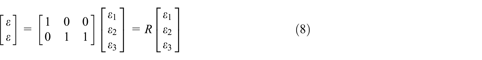
Equation (8) shows the corresponding relationship between the strain equations of the viscoelastic model and the route matrix of the digraph.

The total stress of the Poynting–Thomson model in Figure 3 is denoted as σ, and the stresses of Kelvin units 1, 2, and 3 are denoted as σ₁, σ₂, and σ₃, respectively. The relationship between the total stress σ of the model and the strain ε _i of each Kelvin unit can be determined based on the closed enclosures including the starting points in the digraph G₁ = (V, E). The closed enclosure must satisfy the following condition: the direction of the directed edge intersecting the closed enclosure should point outward. There is a corresponding relationship between them. The extended standard model of the Poynting–Thomson model shown in Figure 3 has two equations that relate the total stress σ and the strain ε _i of each Kelvin unit:

$$\sigma ={\sigma }_1+{\sigma }_2=E_1{\epsilon }_1+{\eta }_1\frac{d{\epsilon }_1}{\mathrm{dt}}+E_2{\epsilon }_2+{\eta }_2\frac{d{\epsilon }_2}{\mathrm{dt}}$$

(9)

$$\sigma ={\sigma }_1+{\sigma }_3=E_1{\epsilon }_1+{\eta }_1\frac{d{\epsilon }_1}{\mathrm{dt}}+E_3{\epsilon }_3+{\eta }_3\frac{d{\epsilon }_3}{\mathrm{dt}}$$

(10)

In the digraph corresponding to the Poynting–Thomson model shown in Figure 4, there are two closed enclosures including the starting point in the digraph G₁ = (V, E). They are as follows: (1) The closed enclosure that intersects the edges e₁ and e₂ and (2) the closed enclosure that intersects the edges e₁ and e₃, as shown in Figure 6.

Figure 6.

Closed enclosures of the digraph G₁ = (V, E).

The enclosure matrix of the digraph G₁ = (V, E) is as follows:

$$E=\left[\begin{array}{ccc}1\hfill & 1\hfill & 0\hfill \\ \multicolumn{1}{c}{1}& 0\hfill & 1\hfill \end{array}\right]$$

(11)

The meaning of the enclosure matrix is as follows. Each row in the matrix E above represents a closed enclosure including the starting point. If the closed enclosure intersects a certain directed edge, the corresponding column of the enclosure matrix is 1, and if the closed enclosure is not intersected, it is 0. As shown in Figure 6, circle ① intersects the edges e₁ and e₂, columns 1 and 2 of the first row of the enclosure matrix E are 1, and the remaining columns of the first row are 0; circle ② intersects the edges e₁ and e₃, columns 1 and 3 of the second row of the enclosure matrix E are 1, and the remaining columns of the second row are 0. The number of rows of the enclosure matrix E is the number of closed enclosures. The number of columns of the enclosure matrix E is the number of edges of the digraph G₁ = (V, E).

Because every closed enclosure of matrix E must intersect every route of matrix R, the dot product of every row vector of matrix E and each row vector of matrix R is 1. When the route matrix R is known, the enclosure matrix E can be obtained by solving the following equation for x (where the element of x can only be 1 or 0):

$$R·x=\begin{array}{ccc}c,\hfill & \mathrm{where}\hfill & c=\left[\begin{array}{c}1\hfill \\ \multicolumn{1}{c}{1}\end{array}\right]\hfill \end{array}$$

(12)

where the nonhomogeneous term c is a column vector with all elements of 1. The number of elements in vector c is the same as the number of independent strain equations of the viscoelastic model, that is, the number of independent routes of digraph G₁ = (V, E).

The solution is as follows:

$$x_1=\left[\begin{array}{c}1\hfill \\ \multicolumn{1}{c}{1}\\ \multicolumn{1}{c}{0}\end{array}\right]\mathrm{or}{x}_2=\left[\begin{array}{c}1\hfill \\ \multicolumn{1}{c}{0}\\ \multicolumn{1}{c}{1}\end{array}\right]$$

(13)

As shown by equations (11) and (13), the first and second rows of the enclosure matrix E are transposes of x₁ and x₂ (i.e. the linearly independent solutions of equation (12)).

At the same time, the stress equations (equations (9) and (10)) of the viscoelastic model can be expressed in matrix form as follows:

$$\left[\begin{array}{c}\sigma \hfill \\ \multicolumn{1}{c}{\sigma }\end{array}\right]=\left[\begin{array}{cccccc}{E}_1\hfill & E_2\hfill & 0\hfill & {\eta }_1\hfill & {\eta }_2\hfill & 0\hfill \\ \multicolumn{1}{c}{E_1}& 0\hfill & E_3\hfill & {\eta }_1\hfill & 0\hfill & {\eta }_3\hfill \end{array}\right]\left[\begin{array}{c}{\epsilon }_1\hfill \\ \multicolumn{1}{c}{{\epsilon }_2}\\ \multicolumn{1}{c}{{\epsilon }_3}\\ \multicolumn{1}{c}{{\stackrel{·}{\epsilon }}_1}\\ \multicolumn{1}{c}{{\stackrel{·}{\epsilon }}_2}\\ \multicolumn{1}{c}{{\stackrel{·}{\epsilon }}_3}\end{array}\right]$$

(14)

Let

$$Y=\left[\begin{array}{ccc}{E}_1\hfill & \hfill & \hfill \\ \multicolumn{1}{c}{}& E_2\hfill & \hfill \\ \multicolumn{1}{c}{}& \hfill & E_3\hfill \end{array}\right]$$

(15)

$$V=\left[\begin{array}{ccc}{\eta }_1\hfill & \hfill & \hfill \\ \multicolumn{1}{c}{}& {\eta }_2\hfill & \hfill \\ \multicolumn{1}{c}{}& \hfill & {\eta }_3\hfill \end{array}\right]$$

(16)

$$d=\left[\begin{array}{c}1\hfill \\ \multicolumn{1}{c}{1}\end{array}\right]$$

(17)

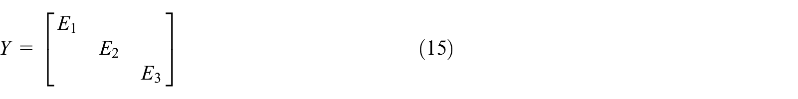
The Y matrix is a diagonal matrix, and the element $Y_{\mathrm{ii}}$ on the diagonal is the modulus of the spring in the ith Kelvin unit. The V matrix is also a diagonal matrix, and the diagonal element $V_{\mathrm{ii}}$ is the viscous coefficient of the damper in the ith Kelvin unit. Vector d is a column vector with all the elements of 1. The number of elements in vector d is the same as the number of independent stress equations of the viscoelastic model, that is, the number of closed enclosures of digraph G₁ = (V, E).

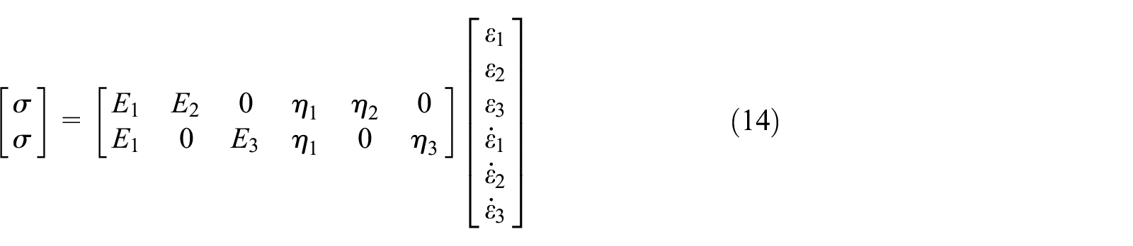
The stress equations (equations (9) and (10)) of the viscoelastic model can be also expressed in matrix form as follows:

$$d\sigma =\left[\begin{array}{cc}\mathrm{EY}\hfill & \mathrm{EV}\hfill \end{array}\right]\left[\begin{array}{c}{\epsilon }_1\hfill \\ \multicolumn{1}{c}{{\epsilon }_2}\\ \multicolumn{1}{c}{{\epsilon }_3}\\ \multicolumn{1}{c}{{\stackrel{·}{\epsilon }}_1}\\ \multicolumn{1}{c}{{\stackrel{·}{\epsilon }}_2}\\ \multicolumn{1}{c}{{\stackrel{·}{\epsilon }}_3}\end{array}\right]$$

(18)

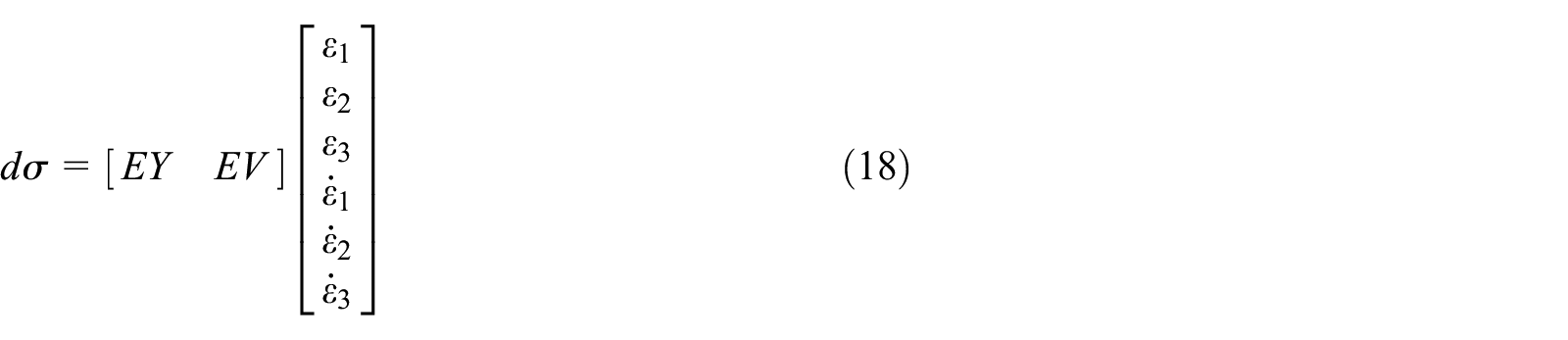
Equation (18) shows the corresponding relationship between the stress equations of the viscoelastic model and the enclosure matrix of the digraph.

Based on the strain equations (equations (2) and (3)) and the stress equations (equations (9) and (10)), the differential relationship between the stress σ and the strain ε of the viscoelastic model can be obtained by eliminating the intermediate variables ε₁, ε₂, and ε₃. The derivation process is as follows.

The first and second derivatives of equations (2) and (3) are calculated (note: for other viscoelastic models, the orders of the derivatives may be different). The relationships between the total strain ε, the first derivative of the strain ε, the second derivative of the strain ε, and the strain ε _i of each Kelvin unit can be written in matrix form as follows:

$$\left[\begin{array}{c}\epsilon \hfill \\ \multicolumn{1}{c}{\epsilon }\\ \multicolumn{1}{c}{\stackrel{·}{\epsilon }}\\ \multicolumn{1}{c}{\stackrel{·}{\epsilon }}\\ \multicolumn{1}{c}{\stackrel{··}{\epsilon }}\\ \multicolumn{1}{c}{\stackrel{··}{\epsilon }}\end{array}\right]=\left[\begin{array}{ccccccccc}1\hfill & 0\hfill & 0\hfill & \hfill & \hfill & \hfill & \hfill & \hfill & \hfill \\ \multicolumn{1}{c}{0}& 1\hfill & 1\hfill & \hfill & \hfill & \hfill & \hfill & \hfill & \hfill \\ \multicolumn{1}{c}{}& \hfill & \hfill & 1\hfill & 0\hfill & 0\hfill & \hfill & \hfill & \hfill \\ \multicolumn{1}{c}{}& \hfill & \hfill & 0\hfill & 1\hfill & 1\hfill & \hfill & \hfill & \hfill \\ \multicolumn{1}{c}{}& \hfill & \hfill & \hfill & \hfill & \hfill & 1\hfill & 0\hfill & 0\hfill \\ \multicolumn{1}{c}{}& \hfill & \hfill & \hfill & \hfill & \hfill & 0\hfill & 1\hfill & 1\hfill \end{array}\right]\left[\begin{array}{c}{\epsilon }_1\hfill \\ \multicolumn{1}{c}{{\epsilon }_2}\\ \multicolumn{1}{c}{{\epsilon }_3}\\ \multicolumn{1}{c}{{\stackrel{·}{\epsilon }}_1}\\ \multicolumn{1}{c}{{\stackrel{·}{\epsilon }}_2}\\ \multicolumn{1}{c}{{\stackrel{·}{\epsilon }}_3}\\ \multicolumn{1}{c}{{\stackrel{··}{\epsilon }}_1}\\ \multicolumn{1}{c}{{\stackrel{··}{\epsilon }}_2}\\ \multicolumn{1}{c}{{\stackrel{··}{\epsilon }}_3}\end{array}\right]$$

(19)

The coefficient matrix of equation (19) is denoted as A:

$$A=\left[\begin{array}{ccccccccc}1\hfill & 0\hfill & 0\hfill & \hfill & \hfill & \hfill & \hfill & \hfill & \hfill \\ \multicolumn{1}{c}{0}& 1\hfill & 1\hfill & \hfill & \hfill & \hfill & \hfill & \hfill & \hfill \\ \multicolumn{1}{c}{}& \hfill & \hfill & 1\hfill & 0\hfill & 0\hfill & \hfill & \hfill & \hfill \\ \multicolumn{1}{c}{}& \hfill & \hfill & 0\hfill & 1\hfill & 1\hfill & \hfill & \hfill & \hfill \\ \multicolumn{1}{c}{}& \hfill & \hfill & \hfill & \hfill & \hfill & 1\hfill & 0\hfill & 0\hfill \\ \multicolumn{1}{c}{}& \hfill & \hfill & \hfill & \hfill & \hfill & 0\hfill & 1\hfill & 1\hfill \end{array}\right]=\left[\begin{array}{ccc}R\hfill & 0\hfill & 0\hfill \\ \multicolumn{1}{c}{0}& R\hfill & 0\hfill \\ \multicolumn{1}{c}{0}& 0\hfill & R\hfill \end{array}\right]$$

(20)

For other viscoelastic models, matrix A is (j + 1) × (j + 1) block matrix, j is the order of the derivative. The blocks on the diagonal of the block matrix are the route matrix R, and the other elements are 0. The coefficient matrix A has (j + 1)× r rows and i × (j + 1) columns, where i is the number of Kelvin units, and r is the rank of route matrix R. In general, A is row full rank matrix, namely, $R(A)=(j+1)r$ .

If equation (19) is regarded as a system of linear equations in terms of ${\epsilon }_1$ , ${\epsilon }_2$ , ${\epsilon }_3$ , ${\stackrel{·}{\epsilon }}_1$ , ${\stackrel{·}{\epsilon }}_2$ , ${\stackrel{·}{\epsilon }}_3$ , ${\stackrel{··}{\epsilon }}_1$ , ${\stackrel{··}{\epsilon }}_2$ , and ${\stackrel{··}{\epsilon }}_3$ , we can obtain the following results:

$$\left[\begin{array}{c}{\epsilon }_1\hfill \\ \multicolumn{1}{c}{{\epsilon }_2}\\ \multicolumn{1}{c}{{\epsilon }_3}\\ \multicolumn{1}{c}{{\stackrel{·}{\epsilon }}_1}\\ \multicolumn{1}{c}{{\stackrel{·}{\epsilon }}_2}\\ \multicolumn{1}{c}{{\stackrel{·}{\epsilon }}_3}\\ \multicolumn{1}{c}{{\stackrel{··}{\epsilon }}_1}\\ \multicolumn{1}{c}{{\stackrel{··}{\epsilon }}_2}\\ \multicolumn{1}{c}{{\stackrel{··}{\epsilon }}_3}\end{array}\right]=\left[\begin{array}{ccc}0\hfill & 0\hfill & 0\hfill \\ \multicolumn{1}{c}{1}& 0\hfill & 0\hfill \\ \multicolumn{1}{c}{-1}& 0\hfill & 0\hfill \\ \multicolumn{1}{c}{0}& 0\hfill & 0\hfill \\ \multicolumn{1}{c}{0}& 1\hfill & 0\hfill \\ \multicolumn{1}{c}{0}& -1\hfill & 0\hfill \\ \multicolumn{1}{c}{0}& 0\hfill & 0\hfill \\ \multicolumn{1}{c}{0}& 0\hfill & 1\hfill \\ \multicolumn{1}{c}{0}& 0\hfill & -1\hfill \end{array}\right]\left[\begin{array}{c}{k}_1\hfill \\ \multicolumn{1}{c}{k_2}\\ \multicolumn{1}{c}{k_3}\end{array}\right]+\left[\begin{array}{c}\epsilon \hfill \\ \multicolumn{1}{c}{\epsilon }\\ \multicolumn{1}{c}{0}\\ \multicolumn{1}{c}{\stackrel{·}{\epsilon }}\\ \multicolumn{1}{c}{\stackrel{·}{\epsilon }}\\ \multicolumn{1}{c}{0}\\ \multicolumn{1}{c}{\stackrel{··}{\epsilon }}\\ \multicolumn{1}{c}{\stackrel{··}{\epsilon }}\\ \multicolumn{1}{c}{0}\end{array}\right]$$

(21)

Equation (21) can also be written as follows:

$$\left[\begin{array}{c}{\epsilon }_1\hfill \\ \multicolumn{1}{c}{{\epsilon }_2}\\ \multicolumn{1}{c}{{\epsilon }_3}\\ \multicolumn{1}{c}{{\stackrel{·}{\epsilon }}_1}\\ \multicolumn{1}{c}{{\stackrel{·}{\epsilon }}_2}\\ \multicolumn{1}{c}{{\stackrel{·}{\epsilon }}_3}\\ \multicolumn{1}{c}{{\stackrel{··}{\epsilon }}_1}\\ \multicolumn{1}{c}{{\stackrel{··}{\epsilon }}_2}\\ \multicolumn{1}{c}{{\stackrel{··}{\epsilon }}_3}\end{array}\right]=\mathrm{null}(A)\times \left[\begin{array}{c}{k}_1\hfill \\ \multicolumn{1}{c}{k_2}\\ \multicolumn{1}{c}{k_3}\end{array}\right]+P.S$$

(22)

where $\mathrm{null}(A^T)$ is the zero space matrix of the coefficient matrix A, k₁, k₂, and k₃ are arbitrary constants, and $P.S$ is any particular solution of equation (19). The particular solution can be constructed in the following way:

$$P.S=F\left[\begin{array}{c}\epsilon \hfill \\ \multicolumn{1}{c}{\stackrel{·}{\epsilon }}\\ \multicolumn{1}{c}{\stackrel{··}{\epsilon }}\end{array}\right],\mathrm{where}F=\left[\begin{array}{ccc}f\hfill & 0\hfill & 0\hfill \\ \multicolumn{1}{c}{0}& f\hfill & 0\hfill \\ \multicolumn{1}{c}{0}& 0\hfill & f\hfill \end{array}\right]$$

(23)

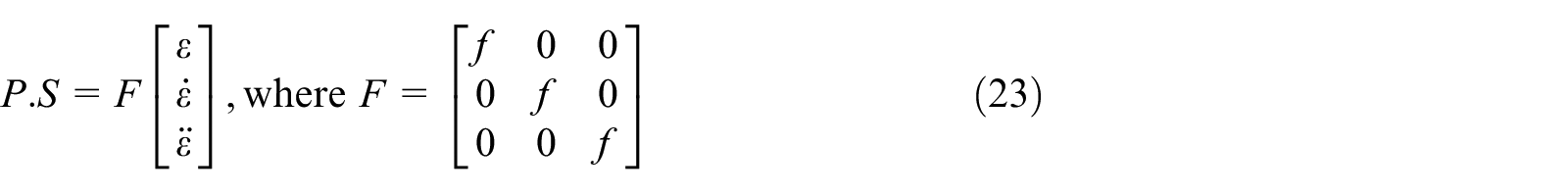
For any other viscoelastic models, F is a (j + 1) × (j + 1) block matrix, j is the order of the derivative. The block on the diagonal of the block matrix is the column vector f, and the other elements are 0. The vector f is the transpose of any row of the enclosure matrix E.

The derivatives of equations (9) and (10) are calculated. The relationship between the total stress σ, the derivative of the total stress σ, the strain ε _i of each Kelvin unit, and the derivatives of strain ε _i can be written in matrix form:

$$\left[\begin{array}{c}\sigma \hfill \\ \multicolumn{1}{c}{\sigma }\\ \multicolumn{1}{c}{\stackrel{·}{\sigma }}\\ \multicolumn{1}{c}{\stackrel{·}{\sigma }}\end{array}\right]=\left[\begin{array}{ccccccccc}{E}_1\hfill & E_2\hfill & 0\hfill & {\eta }_1\hfill & {\eta }_2\hfill & 0\hfill & \hfill & \hfill & \hfill \\ \multicolumn{1}{c}{E_1}& 0\hfill & E_3\hfill & {\eta }_1\hfill & 0\hfill & {\eta }_3\hfill & \hfill & \hfill & \hfill \\ \multicolumn{1}{c}{}& \hfill & \hfill & E_1\hfill & E_2\hfill & 0\hfill & {\eta }_1\hfill & {\eta }_2\hfill & 0\hfill \\ \multicolumn{1}{c}{}& \hfill & \hfill & E_1\hfill & 0\hfill & E_3\hfill & {\eta }_1\hfill & 0\hfill & {\eta }_3\hfill \end{array}\right]\left[\begin{array}{c}{\epsilon }_1\hfill \\ \multicolumn{1}{c}{{\epsilon }_2}\\ \multicolumn{1}{c}{{\epsilon }_3}\\ \multicolumn{1}{c}{{\stackrel{·}{\epsilon }}_1}\\ \multicolumn{1}{c}{{\stackrel{·}{\epsilon }}_2}\\ \multicolumn{1}{c}{{\stackrel{·}{\epsilon }}_3}\\ \multicolumn{1}{c}{{\stackrel{··}{\epsilon }}_1}\\ \multicolumn{1}{c}{{\stackrel{··}{\epsilon }}_2}\\ \multicolumn{1}{c}{{\stackrel{··}{\epsilon }}_3}\end{array}\right]$$

(24)

The coefficient matrix of equation (24) is denoted as B, namely,

$$B=\left[\begin{array}{ccccccccc}{E}_1\hfill & E_2\hfill & 0\hfill & {\eta }_1\hfill & {\eta }_2\hfill & 0\hfill & \hfill & \hfill & \hfill \\ \multicolumn{1}{c}{E_1}& 0\hfill & E_3\hfill & {\eta }_1\hfill & 0\hfill & {\eta }_3\hfill & \hfill & \hfill & \hfill \\ \multicolumn{1}{c}{}& \hfill & \hfill & E_1\hfill & E_2\hfill & 0\hfill & {\eta }_1\hfill & {\eta }_2\hfill & 0\hfill \\ \multicolumn{1}{c}{}& \hfill & \hfill & E_1\hfill & 0\hfill & E_3\hfill & {\eta }_1\hfill & 0\hfill & {\eta }_3\hfill \end{array}\right]=\left[\begin{array}{ccc}\mathrm{EY}\hfill & \mathrm{EV}\hfill & 0\hfill \\ \multicolumn{1}{c}{0}& \mathrm{EY}\hfill & \mathrm{EV}\hfill \end{array}\right]$$

(25)

For any other viscoelastic model, B is a j × (j + 1) block matrix, and j is the order of the derivative. The block on the diagonal of block matrix is EY. The block B_ij (j = i + 1), which is to the right of the diagonal of block matrix B, is EV. The other elements are 0. The coefficient matrix B has j × n rows and i × (j + 1) columns, where n is the rank of enclosure matrix E. In general, B is row full rank matrix, namely, R(B) = j × n.

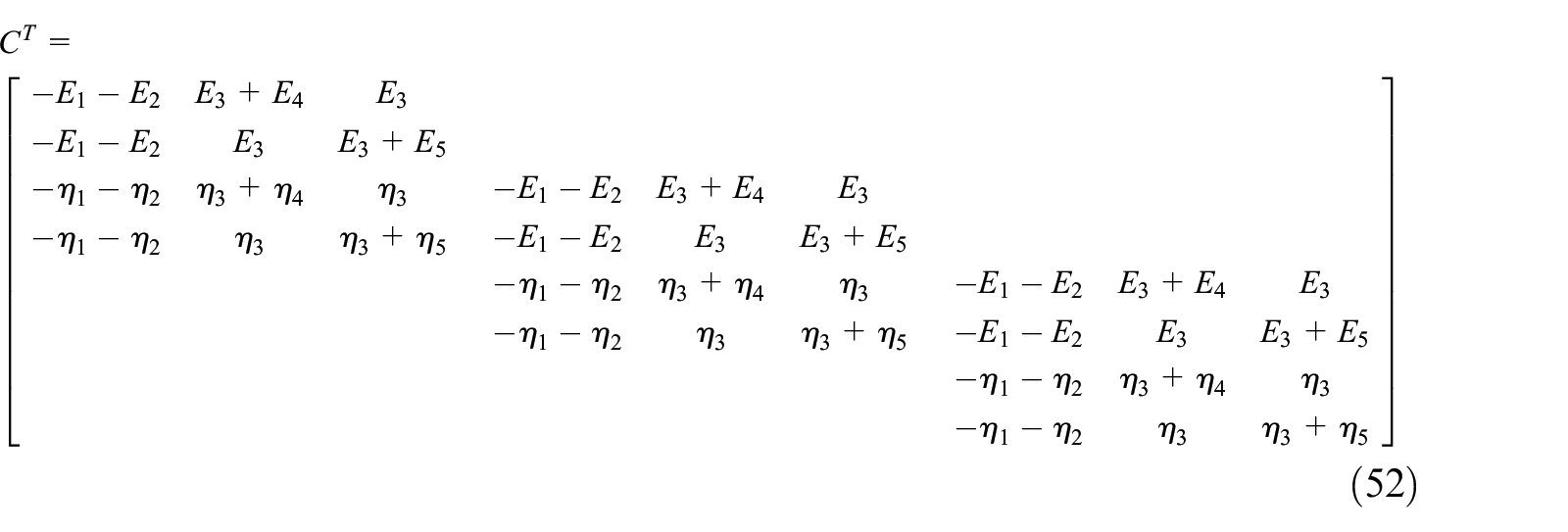
By substituting equation (22) into equation (24), we obtain the following results:

$$\left[\begin{array}{c}\sigma \hfill \\ \multicolumn{1}{c}{\sigma }\\ \multicolumn{1}{c}{\stackrel{·}{\sigma }}\\ \multicolumn{1}{c}{\stackrel{·}{\sigma }}\end{array}\right]=B\times \mathrm{null}(A)\times \left[\begin{array}{c}{k}_1\hfill \\ \multicolumn{1}{c}{k_2}\\ \multicolumn{1}{c}{k_3}\end{array}\right]+B\times P.S$$

(26)

The coefficient matrix of equation (26) is denoted as C, namely,

$$\begin{array}{c}C=B\times \mathrm{null}(A)\hfill \\ =\left[\begin{array}{ccc}\mathrm{EY}\hfill & \mathrm{EV}\hfill & 0\hfill \\ \multicolumn{1}{c}{0}& \mathrm{EY}\hfill & \mathrm{EV}\hfill \end{array}\right]\times \left[\begin{array}{ccc}\mathrm{null}(R)\hfill & 0\hfill & 0\hfill \\ \multicolumn{1}{c}{0}& \mathrm{null}(R)\hfill & 0\hfill \\ \multicolumn{1}{c}{0}& 0\hfill & \mathrm{null}(R)\hfill \end{array}\right]\hfill \\ =\left[\begin{array}{ccc}E\times Y\times \mathrm{null}(R)\hfill & E\times V\times \mathrm{null}(R)\hfill & 0\hfill \\ \multicolumn{1}{c}{0}& E\times Y\times \mathrm{null}(R)\hfill & E\times V\times \mathrm{null}(R)\hfill \end{array}\right]\hfill \\ =\left[\begin{array}{ccc}{E}_2\hfill & {\eta }_2\hfill & 0\hfill \\ \multicolumn{1}{c}{-E_3}& -{\eta }_3\hfill & 0\hfill \\ \multicolumn{1}{c}{0}& E_2\hfill & {\eta }_2\hfill \\ \multicolumn{1}{c}{0}& -E_3\hfill & -{\eta }_3\hfill \end{array}\right]\hfill \end{array}$$

(27)

In equation (27), for any other viscoelastic model, matrix $\mathrm{null}(A^T)$ has i × (j + 1) rows and (i − r) × (j + 1) columns, so matrix C has j × n rows and (i − r) × (j + 1) columns.

Let D denote a block matrix,

$$D=\left[\begin{array}{cc}d\hfill & 0\hfill \\ \multicolumn{1}{c}{0}& d\hfill \end{array}\right]=\left[\begin{array}{cc}1\hfill & 0\hfill \\ \multicolumn{1}{c}{1}& 0\hfill \\ \multicolumn{1}{c}{0}& 1\hfill \\ \multicolumn{1}{c}{0}& 1\hfill \end{array}\right]$$

(28)

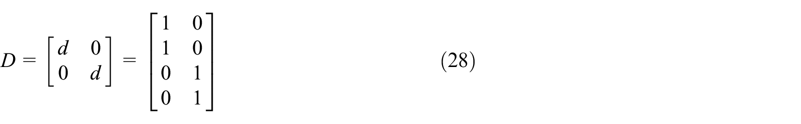
For any other viscoelastic model, D is j × j block matrix, and j is the order of the derivative. The block on the diagonal of the block matrix is vector d, and the other elements are 0.

Equation (26) can also be written in a transposed form as follows:

$${\left[\begin{array}{c}\sigma \hfill \\ \multicolumn{1}{c}{\stackrel{·}{\sigma }}\end{array}\right]}^T\times D^T={\left[\begin{array}{c}{k}_1\hfill \\ \multicolumn{1}{c}{k_2}\\ \multicolumn{1}{c}{k_3}\end{array}\right]}^T\times C^T+{[P.S]}^T\times B^T$$

(29)

To eliminate the arbitrary constants k₁, k₂, and k₃ from equation (29), we can first find the null space matrix $\mathrm{null}(C^T)$ of matrix $C^T$ . The differential relation between the stress σ and strain ε can be obtained by multiplying the terms in equation (29) by the column vector $\mathrm{null}(C^T)$ :

$$\begin{array}{c}{C}^T=\left[\begin{array}{cc}\mathrm{null}{(R)}^T\times Y^T\times E^T\hfill & 0\hfill \\ \multicolumn{1}{c}{\mathrm{null}{(R)}^T\times V^T\times E^T}& \mathrm{null}{(R)}^T\times Y^T\times E^T\hfill \\ \multicolumn{1}{c}{0}& \mathrm{null}{(R)}^T\times V^T\times E^T\hfill \end{array}\right]\hfill \\ \begin{array}{c}=\left[\begin{array}{cccc}{E}_2\hfill & -E_3\hfill & 0\hfill & 0\hfill \\ \multicolumn{1}{c}{{\eta }_2}& -{\eta }_3\hfill & E_2\hfill & -E_3\hfill \\ \multicolumn{1}{c}{0}& 0\hfill & {\eta }_2\hfill & -{\eta }_3\hfill \end{array}\right]\hfill \end{array},\hfill \end{array}$$

(30)

$$\mathrm{null}(C^T)=\left[\begin{array}{c}{E}_3\hfill \\ \multicolumn{1}{c}{E_2}\\ \multicolumn{1}{c}{{\eta }_3}\\ \multicolumn{1}{c}{{\eta }_2}\end{array}\right]$$

(31)

The column vector of $\mathrm{null}(C^T)$ is rewritten as a combination of j vectors a₁, … , a_j (j is the order of the derivative):

$$\mathrm{null}(C^T)=\left[\begin{array}{c}{E}_3\hfill \\ \multicolumn{1}{c}{E_2}\\ \multicolumn{1}{c}{{\eta }_3}\\ \multicolumn{1}{c}{{\eta }_2}\end{array}\right]=\left[\begin{array}{c}{a}_1\hfill \\ \multicolumn{1}{c}{a_2}\end{array}\right]$$

(32)

Thus, the differential constitutive equation of the viscoelastic model is as follows:

$$\left[\begin{array}{cc}{a}_1^T\hfill & a_2^T\hfill \end{array}\right]\left[\begin{array}{cc}d\hfill & 0\hfill \\ \multicolumn{1}{c}{0}& d\hfill \end{array}\right]\left[\begin{array}{c}\sigma \hfill \\ \multicolumn{1}{c}{\stackrel{·}{\sigma }}\end{array}\right]=\left[\begin{array}{cc}{a}_1^T\hfill & a_2^T\hfill \end{array}\right]\left[\begin{array}{ccc}\mathrm{EYf}\hfill & \mathrm{EVf}\hfill & 0\hfill \\ \multicolumn{1}{c}{0}& \mathrm{EYf}\hfill & \mathrm{EVf}\hfill \end{array}\right]\left[\begin{array}{c}\epsilon \hfill \\ \multicolumn{1}{c}{\stackrel{·}{\epsilon }}\\ \multicolumn{1}{c}{\stackrel{··}{\epsilon }}\end{array}\right]$$

(33)

The terms in equation (33) are simplified, expanded, and replaced, and the constitutive equation of the viscoelastic model shown in Figure 3(a) is obtained:

$$\left[\begin{array}{cc}{a}_1^{T}d\hfill & a_2^{T}d\hfill \end{array}\right]\left[\begin{array}{c}\sigma \hfill \\ \multicolumn{1}{c}{\stackrel{·}{\sigma }}\end{array}\right]=\left[\begin{array}{ccc}{a}_1^T\mathrm{EYf}\hfill & (a_1^T\mathrm{EV}+a_2^T\mathrm{EY})f\hfill & a_2^T\mathrm{EVf}\hfill \end{array}\right]\left[\begin{array}{c}\epsilon \hfill \\ \multicolumn{1}{c}{\stackrel{·}{\epsilon }}\\ \multicolumn{1}{c}{\stackrel{··}{\epsilon }}\end{array}\right]$$

(34)

$$\begin{array}{c}(E_2+E_3)\sigma +({\eta }_2+{\eta }_3)\stackrel{·}{\sigma }=(E_1{E}_2+E_1{E}_3+E_2{E}_3)\epsilon \hfill \\ +(E_1{\eta }_2+E_2{\eta }_1+E_1{\eta }_3+E_3{\eta }_1+E_2{\eta }_3+E_3{\eta }_2)\stackrel{·}{\epsilon }+({\eta }_1{\eta }_2+{\eta }_1{\eta }_3+{\eta }_2{\eta }_3)\stackrel{··}{\epsilon }\hfill \end{array}$$

(35)

Letting η₁, η₂, and E₃ be 0, the constitutive equation of the Poynting–Thomson model shown in Figure 2 is as follows:

$$E_2\sigma +{\eta }_3\stackrel{·}{\sigma }=E_1{E}_2\epsilon +(E_1{\eta }_3+E_2{\eta }_3)\stackrel{·}{\epsilon }$$

(36)

Procedure for deriving differential constitutive equation

To facilitate the implementation of this model, the process of determining the correlation coefficient matrix and deriving the differential constitutive equation of an arbitrary linear viscoelastic composite model are summarized as follows:

• (1) All the springs and dashpots in the viscoelastic model are paired into Kelvin units. The viscoelastic model is regarded as a combination of Kelvin units. When there are non-Kelvin units in the model composed of springs and dampers, the non-Kelvin units are extended to Kelvin units first.

• (2) Each Kelvin unit of the viscoelastic model is transformed into a directed edge, and then a directed graph is formed. The incidence matrix M of the digraph G = (V, E) is obtained.

• (3) The linearly independent solutions of the equation Mx = b are determined, and the route matrix R of the digraph G = (V, E) is obtained, where the nonhomogeneous term b represents the route from the starting vertex to the ending vertex.

• (4) The linearly independent solutions of the equation Rx = c are determined, and the enclosure matrix E of the digraph G = (V, E) is obtained, where the nonhomogeneous term c is a column vector with all elements of 1.

• (5) If the rank of the route matrix R is r, the rank of the enclosure matrix E is n, the number of Kelvin units in viscoelastic model is i, and the zero space matrix $\mathrm{null}(C^T)$ of $C^T$ has j × n rows j × n − (i − r) × (j + 1) columns. The zero space matrix $\mathrm{null}(C^T)$ of $C^T$ contains at least one vector that must be satisfied:

$$j·n-(i-r)(j+1)\ge 1$$

(37)

and thus,

$$j\ge \frac{1-r+i}{n+r-i}$$

(38)

Taking j as the smallest positive integer satisfying the equation (38), we can obtain the matrix $C^T$ based on equation (39) and thus obtain $\mathrm{null}(C^T)$ . In general, $C^T$ is (j + 1) × j block matrix,

$$C^T=\underset{j}{\underbrace{\left[\begin{array}{cccc}\mathrm{null}{(R)}^T\times Y\times E^T\hfill & 0\hfill & \cdots \hfill & 0\hfill \\ \multicolumn{1}{c}{\mathrm{null}{(R)}^T\times V\times E^T}& \mathrm{null}{(R)}^T\times Y\times E^T\hfill & \cdots \hfill & 0\hfill \\ \multicolumn{1}{c}{\cdots }& \cdots \hfill & \cdots \hfill & \cdots \hfill \\ \multicolumn{1}{c}{0}& 0\hfill & \cdots \hfill & \mathrm{null}{(R)}^T\times Y\times E^T\hfill \\ \multicolumn{1}{c}{0}& 0\hfill & \cdots \hfill & \mathrm{null}{(R)}^T\times V\times E^T\hfill \end{array}\right]\}}}j+1$$

(39)

• (6) Letting h be a column vector of matrix $\mathrm{null}(C^T)$ , the matrix form of the differential constitutive equation of viscoelastic model is as follows:

$$h^T\times D\times \left[\begin{array}{c}\sigma \hfill \\ \multicolumn{1}{c}{\frac{d\sigma }{\mathrm{dt}}}\\ \multicolumn{1}{c}{⋮}\\ \multicolumn{1}{c}{\frac{d^{j-1}\sigma }{d{t}^{j-1}}}\end{array}\right]=h^T\times B\times F\times \left[\begin{array}{c}\epsilon \hfill \\ \multicolumn{1}{c}{\frac{d\epsilon }{\mathrm{dt}}}\\ \multicolumn{1}{c}{⋮}\\ \multicolumn{1}{c}{\frac{d^j\epsilon }{d{t}^j}}\end{array}\right]$$

(40)

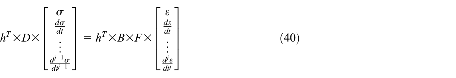
where D is the j × j block matrix, B is the j × (j + 1) block matrix, and F is the (j + 1) × (j + 1) block matrix, defined as follows:

$$D=\underset{j}{\underbrace{\left[\begin{array}{cccc}d\hfill & 0\hfill & \cdots \hfill & 0\hfill \\ \multicolumn{1}{c}{0}& d\hfill & \cdots \hfill & 0\hfill \\ \multicolumn{1}{c}{\cdots }& \cdots \hfill & \cdots \hfill & \cdots \hfill \\ \multicolumn{1}{c}{0}& 0\hfill & \cdots \hfill & d\hfill \end{array}\right]\}}}j$$

(41)

$$B=\underset{j+1}{\underbrace{\left[\begin{array}{ccccc}\mathrm{EY}\hfill & \mathrm{EV}\hfill & \dots \hfill & 0\hfill & 0\hfill \\ \multicolumn{1}{c}{0}& \mathrm{EY}\hfill & \dots \hfill & 0\hfill & 0\hfill \\ \multicolumn{1}{c}{\dots }& \dots \hfill & \dots \hfill & \dots \hfill & \dots \hfill \\ \multicolumn{1}{c}{0}& 0\hfill & \dots \hfill & \mathrm{EY}\hfill & \mathrm{EV}\hfill \end{array}\right]\}}}j$$

(42)

$$F=\underset{j+1}{\underbrace{\left[\begin{array}{ccccc}f\hfill & 0\hfill & 0\hfill & \dots \hfill & 0\hfill \\ \multicolumn{1}{c}{0}& f\hfill & 0\hfill & \dots \hfill & 0\hfill \\ \multicolumn{1}{c}{0}& 0\hfill & f\hfill & \dots \hfill & 0\hfill \\ \multicolumn{1}{c}{\dots }& \dots \hfill & \dots \hfill & \dots \hfill & \dots \hfill \\ \multicolumn{1}{c}{0}& 0\hfill & 0\hfill & \dots \hfill & f\hfill \end{array}\right]\}}}j+1$$

(43)

Calculation example

The differential constitutive equation of a viscoelastic model with 10 springs and dampers shown in Figure 7(a) is quickly determined using the method presented in Section 3.

Figure 7.

(a) Viscoelastic model with 10 springs and dampers, which can be regarded as (b) a model composed of Kelvin units.

The corresponding digraph is shown in Figure 8.

Figure 8.

Digraph corresponding to the viscoelastic model with ten springs and dampers.

The incidence matrix M of the digraph G₂ = (V, E) shown in Figure 8 is as follows:

$$M=\begin{array}{cc}\multicolumn{1}{c}{\left[\begin{array}{ccccc}{e}_1\hfill & e_2\hfill & e_3\hfill & e_4\hfill & e_5\hfill \\ 1\hfill & 1\hfill & 0\hfill & 0\hfill & 0\hfill \\ \multicolumn{1}{c}{-1}& -1\hfill & 1\hfill & 1\hfill & 0\hfill \\ \multicolumn{1}{c}{0}& 0\hfill & 0\hfill & -1\hfill & 1\hfill \\ \multicolumn{1}{c}{0}& 0\hfill & -1\hfill & 0\hfill & -1\hfill \end{array}\right]}& \begin{array}{c}{v}_1\hfill \\ \multicolumn{1}{c}{v_2}\\ \multicolumn{1}{c}{v_3}\\ \multicolumn{1}{c}{v_4}\end{array}\hfill \end{array}$$

(44)

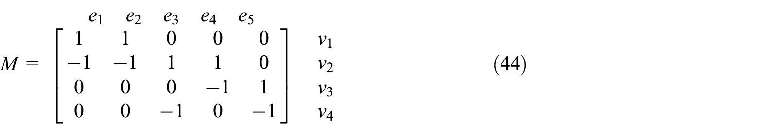
The linearly independent solutions of the equation Mx = b are determined to obtain the route matrix R of the digraph G₂ = (V, E):

$$\left[\begin{array}{ccccc}1\hfill & 1\hfill & 0\hfill & 0\hfill & 0\hfill \\ \multicolumn{1}{c}{-1}& -1\hfill & 1\hfill & 1\hfill & 0\hfill \\ \multicolumn{1}{c}{0}& 0\hfill & 0\hfill & -1\hfill & 1\hfill \\ \multicolumn{1}{c}{0}& 0\hfill & -1\hfill & 0\hfill & -1\hfill \end{array}\right]·x=\left[\begin{array}{c}1\hfill \\ \multicolumn{1}{c}{0}\\ \multicolumn{1}{c}{0}\\ \multicolumn{1}{c}{-1}\end{array}\right]$$

(45)

Three linearly independent solutions are obtained by solving equation (45):

$$x_1=\left[\begin{array}{c}1\hfill \\ \multicolumn{1}{c}{0}\\ \multicolumn{1}{c}{1}\\ \multicolumn{1}{c}{0}\\ \multicolumn{1}{c}{0}\end{array}\right]\mathrm{or}{x}_2=\left[\begin{array}{c}0\hfill \\ \multicolumn{1}{c}{1}\\ \multicolumn{1}{c}{1}\\ \multicolumn{1}{c}{0}\\ \multicolumn{1}{c}{0}\end{array}\right]\mathrm{or}{x}_3=\left[\begin{array}{c}1\hfill \\ \multicolumn{1}{c}{0}\\ \multicolumn{1}{c}{0}\\ \multicolumn{1}{c}{1}\\ \multicolumn{1}{c}{1}\end{array}\right]$$

(46)

The route matrix R of the digraph G₂ = (V, E) is as follows:

$$R={\left[\begin{array}{ccc}{x}_1\hfill & x_2\hfill & x_3\hfill \end{array}\right]}^T=\left[\begin{array}{ccccc}1\hfill & 0\hfill & 1\hfill & 0\hfill & 0\hfill \\ \multicolumn{1}{c}{0}& 1\hfill & 1\hfill & 0\hfill & 0\hfill \\ \multicolumn{1}{c}{1}& 0\hfill & 0\hfill & 1\hfill & 1\hfill \end{array}\right]$$

(47)

The linearly independent solutions of the equation Rx = c are determined to obtain the enclosure matrix E of the digraph G₂ = (V, E):

$$\left[\begin{array}{ccccc}1\hfill & 0\hfill & 1\hfill & 0\hfill & 0\hfill \\ \multicolumn{1}{c}{0}& 1\hfill & 1\hfill & 0\hfill & 0\hfill \\ \multicolumn{1}{c}{1}& 0\hfill & 0\hfill & 1\hfill & 1\hfill \end{array}\right]·x=\left[\begin{array}{c}1\hfill \\ \multicolumn{1}{c}{1}\\ \multicolumn{1}{c}{1}\end{array}\right]$$

(48)

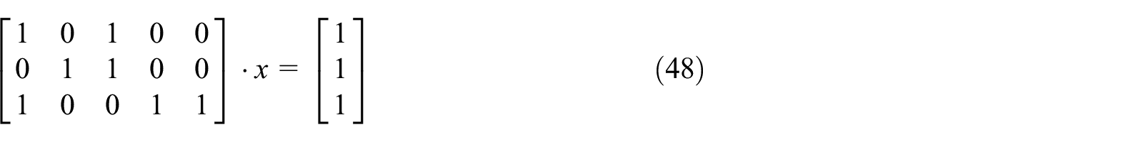
Three linearly independent solutions are obtained by solving equation (48):

$$x_1=\left[\begin{array}{c}1\hfill \\ \multicolumn{1}{c}{1}\\ \multicolumn{1}{c}{0}\\ \multicolumn{1}{c}{0}\\ \multicolumn{1}{c}{0}\end{array}\right]\mathrm{or}{x}_2=\left[\begin{array}{c}0\hfill \\ \multicolumn{1}{c}{0}\\ \multicolumn{1}{c}{1}\\ \multicolumn{1}{c}{1}\\ \multicolumn{1}{c}{0}\end{array}\right]\mathrm{or}{x}_3=\left[\begin{array}{c}0\hfill \\ \multicolumn{1}{c}{0}\\ \multicolumn{1}{c}{1}\\ \multicolumn{1}{c}{0}\\ \multicolumn{1}{c}{1}\end{array}\right]$$

(49)

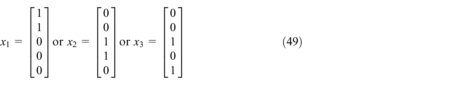
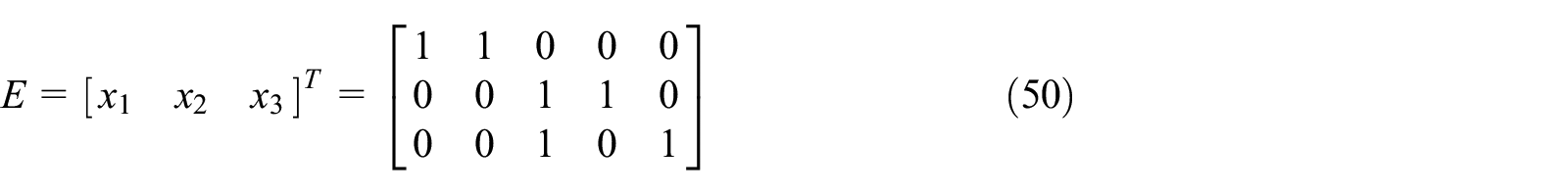
The enclosure matrix E of the digraph G₂ = (V, E) is as follows:

$$E={\left[\begin{array}{ccc}{x}_1\hfill & x_2\hfill & x_3\hfill \end{array}\right]}^T=\left[\begin{array}{ccccc}1\hfill & 1\hfill & 0\hfill & 0\hfill & 0\hfill \\ \multicolumn{1}{c}{0}& 0\hfill & 1\hfill & 1\hfill & 0\hfill \\ \multicolumn{1}{c}{0}& 0\hfill & 1\hfill & 0\hfill & 1\hfill \end{array}\right]$$

(50)

Substituting r = rank(R) = 3, n = rank(E) = 3, i = 5, into equation (38):

$$j\ge \frac{1-r+i}{n+r-i}=\frac{1-3+5}{3+3-5}=3$$

(51)

We can obtain the matrix $C^T$ based on equation (39) by taking j = 3:

$$\begin{array}{c}{C}^T=\hfill \\ \left[\begin{array}{ccc}\begin{array}{ccc}-E_1-E_2\hfill & E_3+E_4\hfill & E_3\hfill \\ \multicolumn{1}{c}{-E_1-E_2}& E_3\hfill & E_3+E_5\hfill \end{array}\hfill & \hfill & \hfill \\ \multicolumn{1}{c}{\begin{array}{ccc}-{\eta }_1-{\eta }_2\hfill & {\eta }_3+{\eta }_4\hfill & {\eta }_3\hfill \\ \multicolumn{1}{c}{-{\eta }_1-{\eta }_2}& {\eta }_3\hfill & {\eta }_3+{\eta }_5\hfill \end{array}}& \begin{array}{ccc}-E_1-E_2\hfill & E_3+E_4\hfill & E_3\hfill \\ \multicolumn{1}{c}{-E_1-E_2}& E_3\hfill & E_3+E_5\hfill \end{array}\hfill & \hfill \\ \multicolumn{1}{c}{}& \begin{array}{ccc}-{\eta }_1-{\eta }_2\hfill & {\eta }_3+{\eta }_4\hfill & {\eta }_3\hfill \\ \multicolumn{1}{c}{-{\eta }_1-{\eta }_2}& {\eta }_3\hfill & {\eta }_3+{\eta }_5\hfill \end{array}\hfill & \begin{array}{ccc}-E_1-E_2\hfill & E_3+E_4\hfill & E_3\hfill \\ \multicolumn{1}{c}{-E_1-E_2}& E_3\hfill & E_3+E_5\hfill \end{array}\hfill \\ \multicolumn{1}{c}{}& \hfill & \begin{array}{ccc}-{\eta }_1-{\eta }_2\hfill & {\eta }_3+{\eta }_4\hfill & {\eta }_3\hfill \\ \multicolumn{1}{c}{-{\eta }_1-{\eta }_2}& {\eta }_3\hfill & {\eta }_3+{\eta }_5\hfill \end{array}\hfill \end{array}\right]\hfill \end{array}$$

(52)

The zero space matrix $\mathrm{null}(C^T)$ of $C^T$ is obtained as follows:

$$\mathrm{null}(C^T)=\left[\begin{array}{c}{\mathrm{E}}_3{\mathrm{E}}_4+{\mathrm{E}}_3{\mathrm{E}}_5+{\mathrm{E}}_4{\mathrm{E}}_5\hfill \\ \multicolumn{1}{c}{{\mathrm{E}}_5{\mathrm{E}}_1+{\mathrm{E}}_5{\mathrm{E}}_2}\\ \multicolumn{1}{c}{{\mathrm{E}}_4{\mathrm{E}}_1+{\mathrm{E}}_4{\mathrm{E}}_2}\\ \multicolumn{1}{c}{{\mathrm{E}}_3{\eta }_4+{\mathrm{E}}_4{\eta }_3+{\mathrm{E}}_3{\eta }_5+{\mathrm{E}}_5{\eta }_3+{\mathrm{E}}_4{\eta }_5+{\mathrm{E}}_5{\eta }_4}\\ \multicolumn{1}{c}{{\mathrm{E}}_1{\eta }_5+{\mathrm{E}}_5{\eta }_1+{\mathrm{E}}_2{\eta }_5+{\mathrm{E}}_5{\eta }_2}\\ \multicolumn{1}{c}{{\mathrm{E}}_1{\eta }_4+{\mathrm{E}}_4{\eta }_1+{\mathrm{E}}_2{\eta }_4+{\mathrm{E}}_4{\eta }_2}\\ \multicolumn{1}{c}{{\eta }_3{\eta }_4+{\eta }_3{\eta }_5+{\eta }_4{\eta }_5}\\ \multicolumn{1}{c}{{\eta }_5{\eta }_1+{\eta }_5{\eta }_2}\\ \multicolumn{1}{c}{{\eta }_4{\eta }_1+{\eta }_4{\eta }_2}\end{array}\right]=\left[\begin{array}{c}{a}_1\hfill \\ \multicolumn{1}{c}{a_2}\\ \multicolumn{1}{c}{a_3}\end{array}\right]$$

(53)

Substituting this into equation (40) yields the following:

$${\left[\begin{array}{c}{a}_1\hfill \\ \multicolumn{1}{c}{a_2}\\ \multicolumn{1}{c}{a_3}\end{array}\right]}^T\left[\begin{array}{ccc}d\hfill & 0\hfill & 0\hfill \\ \multicolumn{1}{c}{0}& d\hfill & 0\hfill \\ \multicolumn{1}{c}{0}& 0\hfill & d\hfill \end{array}\right]\left[\begin{array}{c}\sigma \hfill \\ \multicolumn{1}{c}{\stackrel{·}{\sigma }}\\ \multicolumn{1}{c}{\stackrel{··}{\sigma }}\end{array}\right]={\left[\begin{array}{c}{a}_1\hfill \\ \multicolumn{1}{c}{a_2}\\ \multicolumn{1}{c}{a_3}\end{array}\right]}^T\left[\begin{array}{cccc}\mathrm{EY}\hfill & \mathrm{EV}\hfill & \hfill & \hfill \\ \multicolumn{1}{c}{}& \mathrm{EY}\hfill & \mathrm{EV}\hfill & \hfill \\ \multicolumn{1}{c}{}& \hfill & \mathrm{EY}\hfill & \mathrm{EV}\hfill \end{array}\right]\left[\begin{array}{cccc}f\hfill & 0\hfill & 0\hfill & 0\hfill \\ \multicolumn{1}{c}{0}& f\hfill & 0\hfill & 0\hfill \\ \multicolumn{1}{c}{0}& 0\hfill & f\hfill & 0\hfill \\ \multicolumn{1}{c}{0}& 0\hfill & 0\hfill & f\hfill \end{array}\right]\left[\begin{array}{c}\epsilon \hfill \\ \multicolumn{1}{c}{\stackrel{·}{\epsilon }}\\ \multicolumn{1}{c}{\stackrel{··}{\epsilon }}\\ \multicolumn{1}{c}{\epsilon }\end{array}\right]$$

(54)

$$\begin{array}{c}\left[\begin{array}{ccc}{a}_1^{T}d\hfill & a_2^{T}d\hfill & a_3^{T}d\hfill \end{array}\right]\left[\begin{array}{c}\sigma \hfill \\ \multicolumn{1}{c}{\stackrel{·}{\sigma }}\\ \multicolumn{1}{c}{\stackrel{··}{\sigma }}\end{array}\right]\hfill \\ =\left[\begin{array}{cccc}{a}_1^T\mathrm{EYf}\hfill & (a_1^T\mathrm{EV}+a_2^T\mathrm{EY})f\hfill & (a_2^T\mathrm{EV}+a_3^T\mathrm{EY})f\hfill & a_3^T\mathrm{EVf}\hfill \end{array}\right]\left[\begin{array}{c}\epsilon \hfill \\ \multicolumn{1}{c}{\stackrel{·}{\epsilon }}\\ \multicolumn{1}{c}{\stackrel{··}{\epsilon }}\\ \multicolumn{1}{c}{\stackrel{\dots }{\epsilon }}\end{array}\right]\hfill \end{array}$$

(55)

The vectors d and f are as follows:

$$d=\left[\begin{array}{c}1\hfill \\ \multicolumn{1}{c}{1}\\ \multicolumn{1}{c}{1}\end{array}\right]f=\left[\begin{array}{c}1\hfill \\ \multicolumn{1}{c}{1}\\ \multicolumn{1}{c}{0}\\ \multicolumn{1}{c}{0}\\ \multicolumn{1}{c}{0}\end{array}\right]$$

(56)

If the differential constitutive equation has the following form:

$$p_0\sigma +p_1\stackrel{·}{\sigma }+p_2\stackrel{··}{\sigma }=q_0\epsilon +q_1\stackrel{·}{\epsilon }+q_2\stackrel{··}{\epsilon }+q_3\stackrel{\dots }{\epsilon }$$

(57)

and the values of a₁, a₂, a₃, d, E, Y, V, and f are substituted into equation (55), we can obtain the following:

$$p_0=a_1^{T}d=E_1{E}_4+E_1{E}_5+E_2{E}_4+E_2{E}_5+E_3{E}_4+E_3{E}_5+E_4{E}_5$$

(58)

$$\begin{array}{c}{p}_1=a_2^{T}d=E_1{\eta }_4+E_1{\eta }_5+E_2{\eta }_4+E_2{\eta }_5+E_3{\eta }_4+E_3{\eta }_5+E_4{\eta }_5\hfill \\ +{\eta }_1{E}_4+{\eta }_1{E}_5+{\eta }_2{E}_4+{\eta }_2{E}_5+{\eta }_3{E}_4+{\eta }_3{E}_5+{\eta }_4{E}_5\hfill \end{array}$$

(59)

$$p_2=a_3^{T}d={\eta }_1{\eta }_4+{\eta }_1{\eta }_5+{\eta }_2{\eta }_4+{\eta }_2{\eta }_5+{\eta }_3{\eta }_4+{\eta }_3{\eta }_5+{\eta }_4{\eta }_5$$

(60)

$$q_0=a_1^T\mathrm{EYf}=E_1{E}_3{E}_4+E_1{E}_3{E}_5+E_1{E}_4{E}_5+E_2{E}_3{E}_4+E_2{E}_3{E}_5+E_2{E}_4{E}_5$$

(61)

$$\begin{array}{c}\multicolumn{1}{c}{q_1=(a_1^T\mathrm{EV}+a_2^T\mathrm{EY})f=E_1{E}_3{\eta }_4+E_1{E}_3{\eta }_5+E_1{E}_4{\eta }_5+E_2{E}_3{\eta }_4+E_2{E}_3{\eta }_5+E_2{E}_4{\eta }_5}\\ +E_1{\eta }_3{E}_4+E_1{\eta }_3{E}_5+E_1{\eta }_4{E}_5+E_2{\eta }_3{E}_4+E_2{\eta }_3{E}_5+E_2{\eta }_4{E}_5\hfill \\ +{\eta }_1{E}_3{E}_4+{\eta }_1{E}_3{E}_5+{\eta }_1{E}_4{E}_5+{\eta }_2{E}_3{E}_4+{\eta }_2{E}_3{E}_5+{\eta }_2{E}_4{E}_5\hfill \end{array}$$

(62)

$$\begin{array}{c}\multicolumn{1}{c}{q_2=(a_2^T\mathrm{EV}+a_3^T\mathrm{EY})f=E_1{\eta }_3{\eta }_4+E_1{\eta }_3{\eta }_5+E_1{\eta }_4{\eta }_5+E_2{\eta }_3{\eta }_4+E_2{\eta }_3{\eta }_5+E_2{\eta }_4{\eta }_5}\\ +{\eta }_1{\eta }_3{E}_4+{\eta }_1{\eta }_3{E}_5+{\eta }_1{\eta }_4{E}_5+{\eta }_2{\eta }_3{E}_4+{\eta }_2{\eta }_3{E}_5+{\eta }_2{\eta }_4{E}_5\hfill \\ +{\eta }_1{E}_3{\eta }_4+{\eta }_1{E}_3{\eta }_5+{\eta }_1{E}_4{\eta }_5+{\eta }_2{E}_3{\eta }_4+{\eta }_2{E}_3{\eta }_5+{\eta }_2{E}_4{\eta }_5\hfill \end{array}$$

(63)

$$q_3=a_3^T\mathrm{EVf}={\eta }_1{\eta }_3{\eta }_4+{\eta }_1{\eta }_3{\eta }_5+{\eta }_1{\eta }_4{\eta }_5+{\eta }_2{\eta }_3{\eta }_4+{\eta }_2{\eta }_3{\eta }_5+{\eta }_2{\eta }_4{\eta }_5$$

(64)

Conclusion

Plastic, rubber, asphalt, and other engineering materials exhibit time-dependent mechanical responses, such as creep under constant load, stress relaxation under constant deformation, and delayed strain recovery during unloading. These viscoelastic characteristics of a material have an important influence on its mechanical properties under load. It is very important for engineering applications and theoretical research to establish a suitable model to accurately describe the viscoelastic behaviors of materials. To describe the stress–strain behaviors of viscoelastic materials mathematically, models composed of elastic units, viscous units, and their combination are often used, such as the Maxwell model, Kelvin model, and Burgers model. In general, with the increase in the number of springs and dampers, the viscoelastic characteristics that the model can capture will be closer to those of the actual material. However, with more units of the viscoelastic model, the calculations involved in the constitutive equation become more complex. For a viscoelastic model composed of any number of springs and dampers with arbitrary links, the general form of the differential constitutive equation is derived in this article. The differential constitutive equation of the viscoelastic model can be directly obtained by the operations of the relevant characteristic matrix of the digraph. A procedure suitable for computer programming is summarized. This method has significance for accurately constructing viscoelastic models of practical materials and accurately simulating the viscoelastic characteristics and stress–strain behaviors of engineering materials.