Sage Journals: Discover world-class research

Abstract

This paper presents a mathematical model for studying heat transfer in a spacecraft multi-layered thermal protection system, focusing on material properties and thickness optimization. The heat equation is solved using the immersed finite element method, which efficiently handles material discontinuities at layer interfaces. Simulations are conducted for a three-layer thermal protection system with materials such as carbon composites, ceramics, and insulating foams. Results show the impact of material selection and layer thickness on thermal performance, providing valuable insights for spacecraft design. The study demonstrates the effectiveness of the immersed finite element method for multi-material heat transfer problems in aerospace applications.

Keywords

Mathematical model heat equation with diffusion immersed finite element method multi-layer problem

Introduction

Thermal protection systems (TPS) are vital for ensuring the safety and functionality of structures and devices exposed to extreme thermal environments. These systems play a critical role in regulating heat transfer, preserving structural integrity, and maintaining operational reliability under high thermal loads.¹ TPS applications span various industries, including aerospace, automotive, and energy, where materials and designs must withstand severe temperature fluctuations and intense heat fluxes.² For instance, in the context of spacecraft design and operation, TPS play an indispensable role in enabling missions that involve atmospheric entry, planetary exploration, and high-speed maneuvers. They protect the spacecraft and its payload from the extreme thermal environments encountered during these missions, ensuring both structural integrity and operational safety.³ As space exploration pushes the boundaries of speed, the development of efficient, reliable, and innovative TPSs has become increasingly significant.

Mathematical modeling of heat transfer in TPS provides a powerful tool for understanding and predicting thermal behavior under various scenarios. Among these models is the heat equation which describes the distribution of temperature over time and space and serves as a fundamental tool for studying thermal dynamics in complex systems.^{4, 5} However, solving this equation for multi-layered systems with complex geometries and varying material properties presents computational challenges. In this context, many recent studies have addressed advanced modeling techniques in fluid-based heat transfer, such as fractional rheology in oscillatory ducts,⁶ shear-induced heating in nanoliquids under magnetic fields, and thermophoretic effects in MHD stagnation-point flows,^{7, 8} in addition to non-Fourier approaches like the Cattaneo–Christov theory for capturing nonlocal heat conduction behaviors.⁹ On the other hand, other models tackled solid-state heat conduction in stratified media facing challenges posed by sharp interfacial discontinuities and heterogeneous thermal properties. Other recent studies have addressed thermoelastic and thermal responses in multi-layer materials, emphasizing accurate modeling at interfaces. For instance, Tokovyy et al.¹⁰ and Perkowski et al.¹¹ explored homogenized and multi-layer models for thermal stress and surface deflection, while Huang et al.¹² proposed a macro–micro finite element approach for identifying elastic parameters in ceramic composites. Analytical solutions for multi-layer stress evaluation¹³ and investigations into the impact of porosity on high-temperature behavior¹⁴ further highlight the complexity of these systems.

Numerical modeling of heat transfer in multi-layer materials has been extensively studied using a variety of computational techniques. Traditional finite element methods (FEMs) are widely used due to their flexibility in handling complex geometries; however, they require body-fitted meshes that conform to material interfaces, which can complicate mesh generation for multi-layer domains.^{15, 16} As an alternative, finite volume methods offer good conservation properties and are frequently used in engineering applications, but they may struggle with interface resolution in heterogeneous materials.¹⁷ Furthermore, the extended finite element method was later introduced to address interface discontinuities without mesh conformity by enriching the solution space, but its implementation can become complex and computationally intensive.^{18, 19} More recently, interface-fitted and unfitted approaches have been developed to improve interface handling.²⁰

In this study, immersed finite element (IFE) method is proposed to address challenges faced by the classical numerical techniques. The IFE method is a numerical approach used for solving boundary and interface problems in complex domains, and known for its flexibility in handling complex geometries and discontinuous material properties.^{21, 22} The IFE method eliminates the need for conforming meshes, allowing efficient computation in multi-layered configurations without sacrificing accuracy.²³ By integrating IFE method with advanced computational techniques, this paper explores the heat transfer dynamics in multi-layered TPS, providing insights into the influence of material properties and thicknesses on thermal performance.

In fact, the original concept of immersed methods in general was introduced by Peskin²⁴ in the context of fluid–structure interaction problems, where the immersed boundary method was developed to model the interaction of flexible boundaries with fluid flow. However, the immersed boundary method lacked the rigorous numerical framework for problems with sharp discontinuities. Hence, Li et al.^25–27 extended the idea by introducing the IFE method, which incorporated interface conditions directly into the weak formulation of the FEM. In the IFE method, the computational mesh is independent of the geometry of the interfaces, and the method uses special basis functions to capture discontinuities in the solution and its derivatives. This approach avoids the need for the generation of meshes that are fitted to the interface, making it suitable for problems involving complex and/or multiple interfaces. For more details about the IFE method and its advantages, we refer the reader to the following references.^28–36 Moreover, significant efforts have been made to enhance the accuracy and stability of the IFE method. For instance, Adjerid et al.³⁷ introduced enriched high-degree IFE basis functions, which effectively capture high-order discontinuities at material interfaces, improving the method's precision and reliability. Theoretical studies, including error analysis and convergence investigations have further validated the reliability of the method for practical applications.³⁸ Additionally, adaptive mesh refinement strategies have been also investigated, ensuring accurate solutions with optimized resources.³⁹

The first objective of this study is to develop a mathematical model for multi-layered TPSs using the heat equation as the governing framework. Furthermore, we intend to implement and validate the IFE method for solving the considered model problem, enabling a detailed investigation of the thermal behavior of a spacecraft TPS under various configurations. This includes analyzing the effects of material selection and layer thickness on thermal performance and providing insights into the design and optimization of TPS configurations for enhanced efficiency and reliability. By combining mathematical modeling, advanced numerical techniques, and computational analysis, this work aims to contribute to the ongoing efforts in improving the design and performance of TPSs for various applications, particularly, the spacecraft applications.

This paper is structured as follows. In The mathematical model section, we introduce the mathematical model and governing equations for the TPS. In Solving the model using immersed finite element method section, we detail the implementation of the IFE method. In Implementation of the immersed finite element method section, we discuss the theoretical analysis and computational advantages of IFE method. In Numerical results section, we present the numerical simulations and their results, along with an interpretation of key findings. Finally, in Conclusion section, we conclude the study and outline directions for future research.

The mathematical model

The considered TPS is modeled as a one-dimensional multi-layered structure, composed of M layers and exposed to heat flux on its surface. The heat transfer process within the TPS is governed by the heat equation with diffusion term. Each layer is characterized by unique material properties such as thermal conductivity, density, and specific heat capacity. The model problem, boundary conditions, and initial conditions are as follows.

Governing equation/model

The heat conduction in each layer of the TPS is locally described by the heat equation with diffusion. Hence, at each layer k (with: 1 ≤ k ≤ M), the model is written as follows:

ρ_{k} c_{k} \frac{\partial T_{k}}{\partial t} = \frac{\partial}{\partial x} (β_{k} \frac{\partial T_{k}}{\partial x}), x \in [x_{k - 1}, x_{k}], t > 0,

(2.1)

where as follows:

T_k(x, t) is the temperature in layer k as a function of position x and time t;

ρ_k is the density of material in layer k;

c_k is the specific heat capacity of material in layer k;

β_k is the thermal conductivity of material in layer k;

x_k−₁ and x_k are the boundaries of layer k.

Also, the top boundary of the first layer is x₀ = 0, while the bottom part of the bottom layer is denoted as x_M = L.

Boundary conditions and interface jump conditions

It is essential to define appropriate boundary conditions and interface jump conditions to accurately model the thermal behavior. At the exposed surface (x = 0), a convective heat flux is applied, leading to the following boundary condition:

- β_{1} \frac{\partial T_{1}}{\partial x} |_{x = 0} = q_{conv} - h (T_{1} (0, t) - T_{\infty}),

(2.2)

Where as follows:

q_conv is the applied heat flux;

h is the convective heat transfer coefficient;

T_∞ is the ambient temperature.

Furthermore, at the back surface (x = L, the end of the last layer), we have the following additional boundary condition:

- β_{N} \frac{\partial T_{M}}{\partial x} |_{x = L} = h_{b} (T_{M} (L, t) - T_{\infty}),

(2.3)

where h_b is the back-surface convective heat transfer coefficient.

On the other hand, interface jump conditions need to be set up at the interface between the two-layer guaranteeing the continuity of the solution and the flux. Hence, at the interface between two adjacent layers (x = x_k), continuity of temperature and heat flux are enforced, respectively, as follows:

T_{k} (x_{k}, t) = T_{k + 1} (x_{k}, t),

(2.4a)

and

β_{k} \frac{\partial T_{k}}{\partial x} |_{x = x_{k}} = β_{k + 1} \frac{\partial T_{k + 1}}{\partial x} |_{x = x_{k}} .

(2.4b)

Moreover, the initial temperature distribution in the system is assumed to be uniform and equal to the ambient temperature, providing the following initial condition:

T_{k} (x, 0) = T_{\infty}, x \in [x_{k - 1}, x_{k}], \forall k .

(2.5)

The mathematical model described above is then discretized and solved numerically using the immersed FEM. The multi-layered structure is represented as a single computational domain with discontinuities in material properties handled implicitly. Details of the numerical implementation are presented in Solving the model using immersed finite element method section.

Solving the model using immersed finite element method

To solve the model problem (2.1) for the multi-layered TPS, we opt to use the IFE method. In fact, the IFE method is conveniently suitable for problems involving complex geometries and/or discontinuities in the material properties, since it allows for the representation of multi-material domains on a non-conforming mesh. Hence, in this section, we provide an overview of the IFE method framework, its implementation for the considered model problem, and its advantages for this particular problem.

Overview of the immersed finite element method

The IFE method is useful for solving several engineering and scientific problems, such as problems in material sciences, electromagnetism, and fluid dynamics. In particular, it can be applied to solve the multi-layer TPS model (2.1). In fact, in the standard FEM, the computational mesh is required to conform to the geometric boundaries and material interfaces. In contrast, the IFE method allows the mesh to be independent of the material interfaces, which are embedded within the computational domain. This flexibility simplifies the mesh generation and enables efficient modeling of multi-material systems. Indeed, it makes the IFE method efficient compared to other standard methods, since higher accuracy can be easily obtained using the IFE method with simply coarse mesh. Therefore, the key idea of the IFE method is to modify the standard finite element shape functions to incorporate discontinuities in material properties. These modified shape functions, called IFE shape functions, are constructed to satisfy the interface conditions of continuity in temperature and heat flux.

The immersed finite element space

Let E_h be a regular mesh of size h formed over the domain [0, L], where h is the maximum size of the elements (Figure 1 illustrates the case of two layers—one interface point). Any element containing an interface point α_k is referred to as an interface element, the other elements are referred to as non-interface elements. As illustrated in Figure 2, the interface element E = [h_i, h_i₊₁] can be split as E = E⁺ ∪ E⁻ where E⁺ = [h_i, α] while E⁻ = [α, h_i₊₁].

Figure 1.

A sample mesh on a layer [a, b] with an immersed interface point α.

Figure 2.

A sample interface element.

For the non-interface elements, standard finite element spaces and Lagrange shape functions are used. For the interface element, we develop special shape functions which satisfy the Lagrange nodal value conditions in addition to the interface jump conditions (2.4).

The weak formulation of the proposed IFE method for the heat equation (2.1), applied to the multi-layered TPS, is obtained by multiplying the governing equation by a test function $v \in H_{0}^{1} (Ω)$ and integrating over the computational domain Ω = {∪L_k, k = 1 · · ·, M }.

\int_{Ω} ρ c \frac{\partial T}{\partial t} v d x - \int_{Ω} \frac{\partial}{\partial x} (β \frac{\partial T}{\partial x}) v d x = 0, \forall v (x) \in H_{0}^{1} (Ω),

(3.1)

where

H_{0}^{1} (Ω)

is the space of test functions which are continuous, differentiable, and equal to zero on the boundaries of the domain.

This approach ensures that the solution satisfies the heat equation in an integral sense, accommodating the complexities introduced by the multi-layered structure. The interface conditions are implicitly satisfied by constructing IFE shape functions which incorporate the material discontinuities.

Equation (3.1) can be written also as the sum of integrals over each layer L _k as follows:

\sum_{k = 1}^{M} \int_{L_{k}} ρ_{k} c_{k} \frac{\partial T}{\partial t} v d x + \sum_{k = 1}^{M} \int_{L_{k}} \frac{\partial}{\partial x} (β_{k} \frac{\partial T}{\partial x}) v d x = 0, \forall v (x) \in H_{0}^{1} (Ω) .

(3.2)

Applying integration by parts on each layer L _k of Ω then combining the terms, we obtain

\sum_{k = 1}^{M} \int_{L_{k}} ρ_{k} c_{k} \frac{\partial T}{\partial t} v d x + \sum_{k = 1}^{M} \int_{L_{k}} β_{k} \frac{\partial T}{\partial x} \frac{\partial v}{\partial x} d x = 0, \forall v (x) \in H_{0}^{1} (Ω),

(3.3)

which leads to the IFE method as follows: determining

{\tilde{T}}^{h} \in S_{h, E}^{k}, k = 1, \dots, M

, such that:

{\tilde{T}}^{h}

satisfies (3.3) for all

{\tilde{v}}^{h} \in S_{h, 0}^{k} \subset H_{0}^{1} (Ω)

Construction of immersed finite element shape functions

As mentioned earlier, the computational domain Ω = [0, L] is discretized using a uniform grid. To construct the IFE shape functions, the standard finite element shape functions are modified to satisfy the interface jump conditions. For a given element that intersects a material interface, the shape functions are split into subdomains corresponding to the materials. The following properties are enforced:

Continuity of temperature across the interface (2.4a);

Continuity of heat flux across the interface (2.4b).

The resulting shape functions are piecewise-defined within the intersecting elements and retain standard finite element properties elsewhere.

Temporal discretization

We also perform a uniform discretization in time into τ intervals with time step size denoted as Δt while the discrete time points are denoted as t_n, n = 1, · · ·, τ . The time derivative is discretized using the implicit backward Euler scheme for stability:

\frac{\partial T}{\partial t} \approx \frac{T (x, t_{n + 1}) - T (x, t_{n})}{Δ t},

(3.4)

where T (x, t_n) and T (x, t_n ₊ ₁) are the temperatures (for a given x) at the previous and current time steps, respectively, and Δt is the time step size. The fully discrete system is then solved iteratively for T (x, t_n ₊ ₁) given T (x, t_n).

Advantages of immersed finite element method

The use of the IFE method for the multi-layered TPS problem has several advantages:

Simplicity in mesh generation: The computational mesh does not need to be aligned with the interfaces which highly reduces the mesh generation complexity.

Efficiency in handling the material discontinuities: The method inherently satisfies interface conditions without requiring additional constraints.

Flexibility for complex geometries: The IFE method can be easily extended to handle irregular geometries and heterogeneous material distributions.

Numerical stability: The implicit time-stepping scheme ensures stability for larger time steps, making it suitable for long-duration simulations.

Implementation of the immersed finite element method

The implementation of the IFE method for solving the multi-layered TPS model involves discretizing the computational domain, constructing the IFE shape functions, assembling the system of equations, and solving for the temperature distribution over time.

Construction of the immersed finite element shape functions

The computational domain Ω is discretized into N elements, each defined by a uniform grid spacing Δx. The nodes of the grid are denoted as ${h_{i}}_{i = 0}^{N}$ , where x₀ = 0 and x_N = L, and L is the total length of the TPS. The time domain is discretized into τ time steps with a time step size Δt. For the multi-layered TPS, material properties such as thermal conductivity k, density ρ, and specific heat capacity c are stored as piecewise constant arrays indexed by the spatial domain.

Furthermore, the IFE shape functions are constructed to satisfy the interface conditions. For elements intersecting material interfaces, the shape functions are split into subdomains corresponding to the materials. These functions are defined piece-wisely ensuring both: (i) the continuity of temperature across the interface, and (ii) the continuity of heat flux across the interface, scaled by the thermal conductivity. The resulting shape functions are computed locally for each element and stored for assembly into the global system matrix.

Assembly of the global system

For each element $e \in E$ , the local stiffness matrix $K^{e}$ and local load vector $f^{e}$ are computed as follows:

K_{i j}^{e} = \int_{e} β \frac{\partial ϕ_{i}}{\partial x} \frac{\partial ϕ_{j}}{\partial x} d x + \int_{e} ρ c \frac{ϕ_{j}}{Δ t} \frac{\partial ϕ_{i}}{\partial x} d x,

(4.1)

f_{i}^{e} = \int_{e} ρ c ϕ_{i} \frac{T (x, t_{n})}{Δ t} d x,

(4.2)

where ϕ_i and ϕ_j are the IFE shape functions.

The global system matrix K and the global load vector f are assembled by summing the contributions from all elements:

K = \sum_{e = 1}^{N_{e}} K^{e}, f = \sum_{e = 1}^{N_{e}} f^{e},

(4.3)

where N_e is the number of elements in the mesh. We also note that the boundary conditions are incorporated into the global system matrix and vector.

Hence, the resulting linear system of equations at each time step will be:

K T^{n + 1} = f,

(4.4)

where

T^{n + 1}

is the temperature vector at the next time step (i.e.

T_{i, j}^{n + 1}

). This system is solved using conjugate gradient method with LU factorization.

Furthermore, the temperature is updated iteratively for each time step using the implicit backward Euler scheme:

T^{n + 1} = T^{n} + Δ t K^{- 1} (f - K T^{n}) .

(4.5)

This approach ensures numerical stability, particularly for the large thermal gradients expected in TPS applications.

Numerical implementation

In sum, the numerical implementation can be summarized according to the following steps:

Define the computational domain, material properties, and initial conditions.

Construct the IFE shape functions.

Assemble the global system matrix and load vector.

Apply boundary conditions.

Solve the linear system iteratively for each time step.

Store and visualize the temperature distribution.

Furthermore, to clarify the implementation procedure, a detailed flowchart outlining the computational steps is presented in Figure 3. This diagram illustrates the overall workflow from mesh generation to numerical solution, highlighting how interface conditions are incorporated into the IFE framework.

Figure 3.

Flowchart of the IFE method key implementation steps, for the multi-layer heat conduction problem. IFE: immersed finite element.

Numerical results

In this section, we present numerical simulation results including the temperature distribution and the effects of the material properties and thickness variations on the thermal performance. First, in Figure 4, we present the sample configuration of the considered three-layered TPS, while in Table 1 and Table 2 we display the boundary conditions and the mesh parameters used in the simulation. Additionally, in Table 3 and Table 4, we present the different material properties and the geometry parameters, respectively, which are used in the simulation process under different material configurations.

Figure 4.

A sample configuration of a three-layered TPS. TPS: thermal protection system.

Table 1.

Boundary conditions and initial conditions used in the simulation.

Condition	Value
Surface heat flux (q _s )	1000 W/m²
Back-surface heat transfer coefficient (h)	10 W/m²·K
Initial temperature (T₀)	300 K

Table 2.

Simulation parameters for the multi-layered TPS model.

Parameter	Value
Time step (Δt)	1.0 s
Spatial step (Δx)	0.005 m
Total time (t_max)	5 mim

TPS: thermal protection system.

Table 3.

Material properties of the considered three-layered TPS for the different cases.

Material	Baseline	Case 1	Case 2	Case 3	Case 4
Thermal conductivity (β, W/m·K)	1475.1	600	800	1200	1000
Density (ρ, kg/m³)	1700	2500	2300	1600	2000
Specific heat capacity (c, J/kg·K)	700	1000	950	1200	800

TPS: thermal protection system.

Table 4.

Geometry parameters of the multi-layered TPS model for the different cases.

Parameter	Baseline	Case 1	Case 2	Case 3	Case 4
Total TPS length (L)	0.1 m	0.1 m	0.1 m	0.1 m	0.1 m
Layer 1 thickness (L1)	0.02 m	0.02 m	0.025 m	0.03 m	0.02 m
Layer 2 thickness (L2)	0.03 m	0.04 m	0.03 m	0.02 m	0.03 m
Layer 3 thickness (L3)	0.05 m	0.04 m	0.045 m	0.05 m	0.05 m

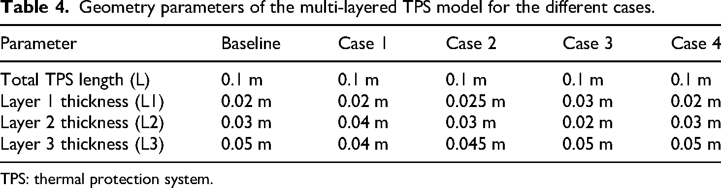
TPS: thermal protection system.

To assess the final temperature profile across the TPS, we first display in Figure 5 the final temperature profile across the TPS. The plot shows the steady-state temperature distribution in the TPS at the end of the simulation for each case, illustrating the effects of material property changes on the thermal performance. We observe that for the baseline case as well as for the cases of materials 2, 3, and 4 (respectively characterized by lower β₂, lower β₃, and higher ρ₃/c₃), the temperature gradient is smooth, with a steady decrease from the high-temperature boundary to the insulated side. The temperature drop across each layer reflects the thermal conductivities of the materials. Specifically, the middle layer, with the highest thermal conductivity, allows for more rapid heat transfer, resulting in a smaller temperature drop compared to the outer layers. Conversely, in the first case of material where β₁ is higher, increasing the thermal conductivity of the first layer reduces the temperature drop across it, enabling heat to penetrate more efficiently into the subsequent layers and raising their temperatures.

Figure 5.

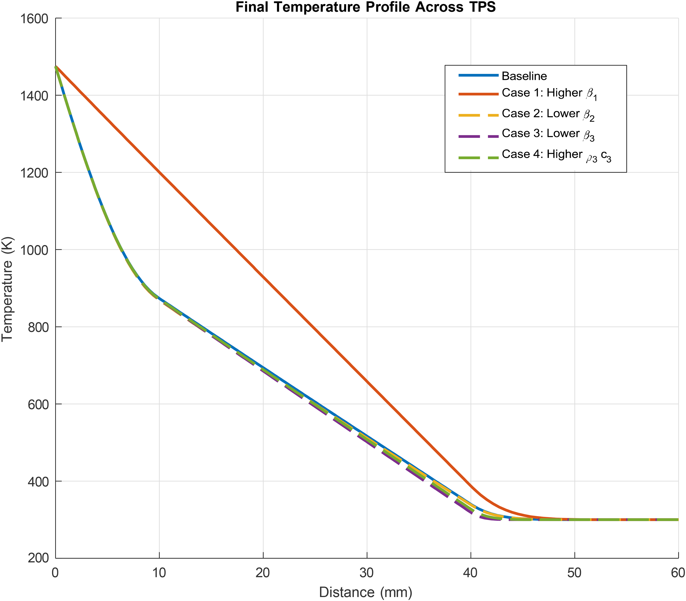
Final temperature profile across the TPS for the different cases. TPS: thermal protection system.

Figure 6 displays the temperature vs. time graphs for specific locations, such as the boundaries of the surface and layers. The graphs provide detailed information on the dynamics of heat penetration in the various test cases, revealing the significant influence of the material properties and configurations on the performance of the TPS. For the baseline case, the temperature gradient is smooth, with a steady decrease from the high-temperature boundary to the insulated side. The temperature drop across each layer reflects the thermal conductivities of the materials, where the middle layer, with the highest thermal conductivity, allows for more rapid heat transfer, resulting in a smaller temperature drop compared to the outer layers. In Case 1, where the first layer has a higher thermal conductivity (β₁), the temperature drop across this layer is reduced, allowing the heat to penetrate more efficiently into the subsequent layers and increasing their temperatures. In Case 2, reducing the thermal conductivity of the middle layer (β₂) creates a significant temperature drop across it (due to heat transfer resistance) which enhances thermal insulation but raises the temperature of the first layer. In Case 3, the lower thermal conductivity of the third layer (β₃) increases its insulating properties, causing the temperature to remain higher in the inner layers, while the final temperature on the insulated side is lower than in other cases. Finally, in Case 4, with a higher density and specific heat capacity (ρ₃ and c₃) for the third layer, the heat transfer process is delayed, resulting in a slightly flatter temperature gradient as the material absorbs and stores more heat without significantly increasing its temperature.

Figure 6.

Temperature variation with time at different levels of the three-layered TPS. TPS: thermal protection system.

Besides, the surface plots shown in Figure 7 show the dynamic interaction between thermal conductivity, density, and heat capacity. These plots provide a dynamic view of how the temperature evolves over time across the TPS. The following main observations are identified from the analysis of the cases. For the baseline case, the temperature rises rapidly near the high-temperature boundary and propagates through the layers over time. The surface clearly reflects the impact of thermal diffusivity, with the middle layer allowing faster temperature changes. In Case 1 (Higher β₁), the heat propagates faster through the first layer due to the higher thermal conductivity, leading to a more significant rise in temperature in the subsequent layers early in the simulation. For Case 2 (Lower β₂), the temperature gradient across the middle layer is steeper compared to the baseline, significantly slowing heat transfer and delaying the temperature rise in the third layer. In Case 3 (Lower β₃), the third layer acts as a more effective insulator, reducing the heat reaching the insulated side and showing a slower temperature increase near the insulated boundary. Finally, for Case 4 (Higher ρ₃ and c₃), the higher heat capacity of the third layer delays heat propagation through it, with the surface plot illustrating the third-layer acting as a thermal buffer, absorbing heat while maintaining a flatter gradient.

Figure 7.

Surface plots of the temperature variation with time and position in the TPS. TPS: thermal protection system.

In conclusion, we can synthesize our observations in the following main points:

- High thermal conductivity accelerates heat propagation;

- Low conductivity increases the temperature gradient, enhancing insulation;

- High density and heat capacity slow down heat transfer, acting as thermal buffers.

Comparative study

Compared to other methods, the IFE method shows efficiency in handling the discontinuity. For instance, a comparison with the results reported in^{40, 41} demonstrates comparable or improved accuracy in key metrics. For example, in the multi-layer benchmark case, our IFE method yielded an error with L²−norm of 2.1 × 10 ⁻ ³ that closely matched the accuracy reported by SCTBEM while achieving smooth temperature and flux profiles across discontinuous interfaces. Additionally, the IFE method supports non-conforming meshes, making it more adaptable to complex geometries and interface evolutions that are less tractable for boundary-only methods.

Finally, in Figure 8, an additional test case is provided, which combines both a higher number of layers (five-layer configuration) and a comparative study of the proposed IFE method versus the classical FEM (using body-fit mesh). This comparison highlights the IFE method's ability to maintain accuracy while offering greater flexibility in handling complex multi-layer geometries without requiring mesh conformity.

Figure 8.

Temperatures profiles obtained using classical FE vs. IFE methods in a five-layer medium. IFE: immersed finite element.

Practical considerations on layer thickness and material gradients

While the multi-layer configurations and thicknesses employed in the numerical experiments were primarily chosen to demonstrate the accuracy and robustness of the IFE method, the selected dimensions may exceed those typically encountered in practical TPS. For instance, in aerospace applications, TPS coatings are often limited to a few millimeters in thickness to satisfy weight and space constraints. A promising direction in this context is the use of functionally graded materials (FGMs), which feature a gradual variation in thermal properties across their thickness. Such materials, like ZrO₂−NiCr alloy-based FGMs, are already being developed and tested for aerospace and hypersonic vehicle applications due to their ability to withstand steep thermal gradients while maintaining mechanical stability. The IFE framework is particularly well-suited for modeling FGMs, as it accommodates spatially varying material properties without requiring interface-fitted meshes. One possible extension of this work is to incorporate FGMs with realistic geometries and gradation profiles into simulations to further enhance the engineering relevance of the methodology.

Implications for thermal protection system design

The generated figures collectively illustrate the effectiveness of different material configurations in mitigating thermal loads. This approach enables engineers to design tailored TPS solutions based on mission-specific requirements. The surface plots and steady-state profiles provide complementary insights into the dynamic and equilibrium thermal behavior, offering a comprehensive understanding of the system's performance. As a result, we can extract the following conclusions and interpretations of the current study on TPS design. The choice of materials with specific thermal properties significantly impacts the performance of the TPS. A high β material is suitable for rapid heat dissipation in regions where overheating is critical, while low k materials provide insulation. Balancing layer thicknesses can optimize the TPS's thermal performance; for instance, increasing the thickness of an insulating layer can improve thermal protection but at the cost of weight and bulk. The transient analysis highlights how materials’ heat capacity and density affect temperature evolution, which is crucial for applications where the TPS must withstand short-term, high-intensity thermal loads, such as during reentry phases.

Conclusion

In conclusion, this study demonstrates the potential of the IFE method as an effective tool for analyzing and designing multi-layered TPSs. By incorporating realistic material properties and solving the heat equation in a computationally efficient manner, the proposed approach provides valuable insights into the thermal performance of different TPS configurations. The findings highlight the importance of carefully selecting material properties and optimizing layer thicknesses to achieve the desired balance between insulation, weight, and thermal dissipation. Additionally, the dynamic thermal behavior observed with the transient conditions highlights the importance of considering time-dependent factors in the TPS design. Future work may consist in extending the current one-dimensional IFE framework to higher dimensions, addressing challenges such as interface basis construction, accurate integration over cut elements, and maintaining stability in complex geometries. It may also consist in generalizing this computational methodology by incorporating more complex boundary conditions and taking into account nonlinear material behaviors, which would enhance its applicability to advanced aerospace applications. Additionally, exploring the use of the discontinuous Galerkin method^{42, 43} could provide further flexibility and accuracy in handling the interface conditions and capturing localized phenomena within the TPSs.

Footnotes

ORCID iD

Mohamed Ben-Romdhane

Author contribution

The author solely carried out the conceptualization, methodology development, software implementation, analysis, writing, and revision of the manuscript.

Funding

The author received no financial support for the research in this article.

Declaration of conflicting interests

The author declared no potential conflicts of interest with respect to the research, authorship, and/or publication of this article.

Data availability statement

No external data was used for the research described in the article.

References

Hurwitz

. Thermal Protection Systems (TPSs). In: Encyclopedia of Aerospace Engineering. Online Library: Materials Technology Structural Materials, Wiley, 15 December 2010.

Peluchon

Gallice

Mieussens

. Development of numerical methods to simulate the melting of a thermal protection system. J Comput Phys 2022; 448: 110753.

Wang

, et al. Thermal analysis and thermal management of high power density electric motors for aircraft electrification. Appl Therm Eng 2025; 260: 125006.

Sun

Zeng

, et al. An immersed multi-material arbitrary Lagrangian–Eulerian finite element method for fluid–structure-interaction problems. Comput Methods Appl Mech Eng 2024; 432: 117398.

Wang

Cai

. Modeling the effects of individual layer thickness and orientation on the tri- bocorrosion behavior of Al/Cu nanostructured metallic multilayers. Wear 2021; 477: 203849.

Yasir

Ahmed

Aldosari

, et al. Fractionized based rheological features of transient motion of Walter’s B fluid in a rectangular oscillatory duct with cosine and sine oscillations. J Comput Design Eng 2025; 12: 205–220.

Ahmed

Khattak

Alrihieli

, et al. Shear forces heat generation in MHD uniform flow of nanoliquid across a stretchable surface through Darcy medium. ZAMM - J Appl Math Mech / Zeitschrift für Angewandte Mathematik und Mechanik 2024; 105: e202400450.

Ahammad

Ahmed

Alhowaity

, et al. Convective transport via thermophoresis and Brownian forces in MHD Hiemenz stagnation-point flow. Int J Mod Phys B 2022; 36: 2250203.

Zhang

Ahmed

Naveed Khan

, et al. Swirling flow of fluid containing (SiO₂) and (MoS₂) nanoparticles analyze via Cattaneo-Christov theory. J Appl Biomaterials Functional Materials 2022; 20: 22808000221094685.

10.

Tokovyy

Kulchytskyi-Zhyhailo

Huang

. Thermostressed analysis of multilayer elastic spherical vessels using the homogenized and multilayer models. J Therm Stresses 2025, Published online: 20 Mar 2025.

11.

Perkowski

Kulchytsky-Zhyhailo

Matysiak

, et al. Thermal surface deflection of a medium with multilayer coatings. Int J Mech Sci 2025; 287: 109984.

12.

Huang

Rong

Jiang

, et al. Inverse identification of constituent elastic parameters of ceramic matrix composites based on macro–micro combined finite element model. Aerospace 2024; 11: 936.

13.

Tokovyy

Kulchytskyi-Zhyhailo

. Analytical evaluation of the elastic stresses in a multilayer spherical pressure vessel. Int J Pressure Vessels Piping 2024; 212, Part B, 105354.

14.

Huang

Jiang

Rong

, et al. Effect of porosity on high-temperature tensile properties of 2D woven C/SiC with hole-edge densification structure. Aerospace Sci Technol 2025; 162: 110247.

15.

Zienkiewicz

Taylor

Fox

. The Finite Element Method for Solid and Structural Mechanics. Seventh Edition, Elsevier, 2014.

16.

Reddy

. An Introduction to the Finite Element Method. 4th ed. McGraw-Hill Education, 2019.

17.

Cebula

Taler

. Finite Volume Method in Heat Conduction. In: Hetnarski

(ed.) Encyclopedia of Thermal Stresses. Dordrecht: Springer, 2014, pp. 1645–1658.

18.

Bakalakos

Kalogeris

Papadopoulos

. An extended finite element method formulation for modeling multi-phase boundary interactions in steady state heat conduction problems. Composite Struct 2021; 258: 113202.

19.

Fries

Belytschko

. The extended/generalized finite element method: an overview of the method and its applications. Int J Numer Methods Eng 2010; 84: 253–304.

20.

Hansbo

. An unfitted finite element method, based on Nitsche’s method, for elliptic interface problems. Comput Methods Appl Mech Eng 2002; 191: 5537–5552.

21.

Adjerid

Ben-Romdhane

Lin

. Higher degree immersed finite element methods for second-order elliptic interface problems. Int J Numer Anal Model 2014; 11: 541–566.

22.

Adjerid

Ben-Romdhane

Lin

. Higher degree immersed finite element spaces constructed according to the actual interface. Comput Math Appl 2018; 75: 1868–1881.

23.

Ben-Romdhane

Adjerid

Lin

. Higher-order immersed finite element spaces for second-order elliptic interface problems with quadratic interface. Adv Appl Math Matics 2014, 87: 171–178.

24.

Peskin

. Flow patterns around heart valves: a numerical method. J Comput Phys 1972; 10: 252–271.

25.

. The immersed interface method using a finite element formulation. Applied Numer Math 1998; 27: 253–267.

26.

Lin

. New Cartesian grid methods for interface problems using the finite element formulation. Numer Math 2003; 96: 61–98.

27.

Lin

, et al. An immersed finite element space and its approximation capability. Numer Methods Partial Differential Eq 2004; 20: 338–367.

28.

Adjerid

Lin

. Higher-order immersed discontinuous Galerkin methods. Int J Information Syst Sci 2007; 3: 558–565.

29.

Adjerid

Lin

. A pth-degree immersed finite element method for boundary value problems with discontinuous coefficients. Appl Numer Math 2009; 59: 1303–1321.

30.

Camp

Lin

, et al. Quadratic immersed finite element spaces and their approximation capabilities. Adv Comput Math 2006; 24: 81–112.

31.

Gong

. Immersed-interface finite-element methods for elliptic interface problems with non-homogeneous jump conditions. SIAM J Numer Anal 2008; 46: 472–495.

32.

Lin

. Approximation capability of a bilinear immersed finite element space. Numer Methods Partial Differ Equ 2008; 24: 1265–1300.

33.

Lin

. Immersed finite element methods for elliptic interface problems with non-homogeneous jump conditions. Int J Numer Anal Model 2011; 8: 284–301.

34.

Lin

Zhang

. Immersed finite element methods for parabolic equations with moving interface. Numer Methods Partial Differential Eq 2013; 29: 619–646.

35.

Kafafy

Lin

, et al. 3-D Immersed finite element methods for electric field simulation in composite materials. Int J Numerical Methods Eng 2005; 64: 904–972.

36.

Lin

Rogers

, et al. A rectangular immersed finite element method for interface problems. Adv Comput: Theory and Practice 2001; 7: 107–114.

37.

Adjerid

Babuska

Guo

, et al. An enriched immersed finite element method for interface problems with nonhomogeneous jump conditions. Comput Methods Appl Mech Eng 2023; 404: 115770.

38.

Adjerid

Lin

Meghaichi

. A unified immersed finite element error analysis for one-dimensional interface problems. Bit Numer Math 2024; 64: Article 13.

39.

Lai

. Adaptive mesh refinement for elliptic interface problems using the non-conforming immersed finite element method. Int J Numer Anal Model 2011; 8: 466–483.

40.

Jing

. SCTBEM: A scaled coordinate transformation boundary element method with 99-line MATLAB code for solving Poisson’s equation. Comp Phys Commun 2024; 300: 109185.

41.

Jing

Ren

, et al. A novel SCTBEM with inversion-free Pad´e series expansion for 3D transient heat transfer analysis in FGMs. Comp Methods Appl Mech Eng 2025; 433, Part B, 117546.

42.

Baccouch

Temimi

Ben-Romdhane

. Optimal error estimates and superconvergence of an ultra weak discontinuous Galerkin method for fourth-order boundary-value problems. Appl Numer Math 2019; 137: 91–115.

43.

Temimi

Ben-Romdhane

. A highly accurate discontinuous Galerkin method for solving nonlinear Bratu’s problem. Alexandria Eng J 2024; 95: 50–58.

Immersed finite element method for heat transfer analysis in multi-layered thermal protection systems

Abstract

Keywords

Introduction

The mathematical model

Governing equation/model

Boundary conditions and interface jump conditions

Solving the model using immersed finite element method

Overview of the immersed finite element method

The immersed finite element space

Construction of immersed finite element shape functions

Temporal discretization

Advantages of immersed finite element method

Implementation of the immersed finite element method

Construction of the immersed finite element shape functions

Assembly of the global system

Numerical implementation

Numerical results

Comparative study

Practical considerations on layer thickness and material gradients

Implications for thermal protection system design

Conclusion

Footnotes

ORCID iD

Author contribution

Funding

Declaration of conflicting interests

Data availability statement

References