Sage Journals: Discover world-class research

Abstract

Solar power is one renewable energy source that has great promise. Photovoltaic systems are becoming increasingly popular. Using maximum power point tracker technologies is essential for maximizing the amount of power that can be harvested from a solar system. The variability of the highest power point of a solar system is thought to be caused by the interaction of external elements with the system. In light of the foregoing, the study's overarching goal is to figure out how to use an innovative fuzzy logic controller to track a boost converter-based photovoltaic system's peak power point. We use the fuzzy logic controller to make the system more dynamically sensitive to changes in ambient temperature, quick and moderate variations in irradiance, and other environmental factors. The major objective of this research is to improve the fuzzy logic controller's scaling factors and membership functions. There is a correlation between these features and the controller's accuracy, stability, and speed. For the concept of optimization to be executed well, the cutting-edge metaheuristic method known as Arctic puffin optimization was employed. Arctic Puffin Optimization draws its motivation from nature. Comparisons and analyses with other effective optimization algorithms, such as particle swarm optimization and gray wolf optimizer, have shown that Arctic Puffin Optimization outperforms these other optimization procedures when it comes to fuzzy logic controller tuning. Using the MATLAB/Simulink R2020a environment, we test each method for tracking accuracy, efficiency, response time, transient overshoot, and steady-state ripple. A broad variety of weather conditions was used to conduct the investigation. The Arctic puffin optimization-based fuzzy maximum power point tracker controller's tracking efficacy was consistently over 99.8% in all the conditions investigated, according to the simulation findings.

Keywords

Sustainable energy green energy sources PV systems MPPT strategies FLC APO optimization approaches

Introduction

Background and literature

In contemporary times, renewable energy resources have emerged as a crucial component of the electrical generation system. As a result of their inherent characteristics, these sources do not generate any form of pollution or emissions that might harm the environment. Additionally, they possess an inexhaustible supply, operate in a tranquil manner, and are very simple to maintain.^1,2 Aligned with the prevailing worldwide trend of decarbonization, which aims to address the catastrophic problem of climate change and the ongoing depletion of fossil fuel resources. The use of photovoltaic (PV) energy as an alternative to conventional energy sources has garnered significant attention in regions characterized by abundant solar irradiation. Unfortunately, the suboptimal conversion efficiency of PV modules significantly diminishes the cost-effectiveness of PV systems, while adversely impacting the overall energy production of such systems.

Solar PV modules have the capacity to generate the most amount of electricity to the load while operating at their optimal operating point. The term “Maximum Power Point” (MPP) is a widely used phrase that refers to a certain operational state. The power output of a PV module is determined by the product of voltage and current at the highest power point, which is influenced by the ambient temperature and degree of irradiation. The open circuit voltage of a PV module exhibits considerable variability as a result of fluctuations in irradiation. However, the short circuit current of the module demonstrates a direct proportionality to the degree of irradiance and experiences a notable decrease as irradiation levels decline. Conversely, an increase in temperature leads to a little rise in the short-circuit current, while causing a substantial decrease in voltage.

In summary, it can be shown that an increase in irradiance leads to a corresponding rise in the short circuit current. Conversely, an increase in temperature results in a decrease in the open circuit voltage. These variations in current and voltage have a significant influence on the output power of the PV module. The absence of a coupling device between the PV module and the load results in suboptimal functioning of the system, as it fails to achieve its MPP due to the fluctuation in output power. Hence, it is imperative to provide effective and efficient tracking of the MPP of a PV system by the utilization of a robust maximum power point tracker (MPPT).

It is noteworthy to mention that several research techniques have been developed to optimize the power production of solar panels under varying environmental conditions. Furthermore, it is crucial to address certain challenges that arise in the context of PV systems, including the mitigation of unwanted oscillations in the vicinity of the MPP, the enhancement of resilience against load fluctuations, and the management of weather-related changes. In the field of tracking, many strategies have been categorized into three main groups: classical techniques, soft computing approaches, and hybrid methods.

The conventional methodologies encompass fractional short circuit current,³ fractional open circuit voltage,⁴ sliding mode control,^5,6 incremental conductance,⁷ hill climbing (HC),⁸ perturb and observe (P&O),^9,10 and modified P&O.^11,12 Despite the long-standing utilization of the P&O technique, scholarly investigations have revealed its limitations in accurately monitoring the MPP amid sudden fluctuations in solar irradiance.¹³ These approaches provide the advantage of being very simple to apply; nevertheless, they are characterized by sluggish convergence and lower levels of accuracy.

In contrast, Soft-computing methods rely on various optimization algorithms for their functioning. These algorithms include differential evolution-based MPPT,¹⁴ flower-pollination algorithm,¹⁵ slap-swarm algorithm,¹⁶ firefly algorithm,¹⁷ artificial bee colony (ABC),¹⁸ cuckoo-search algorithm,¹⁹ the whale-optimization algorithm (WOA),²⁰ dragonfly optimization,²¹ particle-swarm optimization (PSO),²² glow worm swarm,²³ ant colony,^24,25 and bee colony.^26,27 Additionally, Soft-computing methods also incorporate algorithms that leverage artificial intelligence techniques such as fuzzy logic^28–34 and neural networks.^35–37 In Prajapati and Fernandez,³⁴ various types of membership functions (MFs) were applied to a fuzzy logic controller (FLC) for a solar PV array. The results revealed that the triangular and trapezoidal functions yielded lower error rates compared to the Gaussian function, demonstrating the superiority of the triangular and trapezoidal functions over the Gaussian.

It is worth mentioning that the soft-computing algorithms have the advantage of being easily implementable on embedded devices, although with a relatively slower convergence rate.

Hybrid power systems, which have been subject to assessment with respect to control schemes using neural networks, particle swarm optimization, or fuzzy logic, sometimes make use of MPPT controllers. Hybrid methodologies that incorporate a combination of conventional and soft computing methods, including PSO-P&O,^38–44 PSO-HC,⁴⁵ PSO-PI,⁴⁶ gray wolf optimizer (GWO)-P&O,⁴⁷ and ANN-P&O,⁴⁸ have been employed.

Research contribution highlights

This study explores the attainment of the MPP of a system through the utilization of a tracking system that operates on the principles of FLC. The objective of this study is to effectively establish the optimal parameters of the fuzzy controller, including MFs and gain factors, in order to achieve the MPP of the system under varied climatic conditions. The primary concern is addressing and minimizing certain challenges, including the oscillation observed around the steady state, the presence of steady-state inaccuracy, and enhancing the overall efficiency of the tracking system. The system's robustness is evaluated across various scenarios, including constant solar irradiance and temperature (referred to as standard testing conditions or STC), constant solar irradiance with rapid temperature changes, rapid variations in irradiance with constant temperature, and simultaneous rapid variations in both irradiance and temperature. Furthermore, the aforementioned three situations are replicated, however with a gradual modulation of temperature and/or irradiance. The below enumeration comprises the primary contributions that may be derived from this corpus of work:

Enhancing the performance of power tracking technique of PV system using FLC based on recently developed meta-heuristic natural inspired optimization technique called Arctic Puffin Optimization (APO) to select the optimal MFs and gain factors. Different climatical conditions are exposed to evaluate its robustness.

The paper is organized as follows: Following the introductory remarks presented in the first section 1. The second section provides a comprehensive exposition of the model employed for the PV system under investigation. The third section provides an elucidation of the FLC system, which serves as the MPPT mechanism. The fourth section provides an explanation of the APO technique suggested for the purpose of optimizing the fuzzy controller MPPT algorithm. The mathematical formulation of the optimization strategy is presented in the fifth section. The findings, analyses, and comparisons are presented in the sixth section. The seventh section serves as the concluding segment of the study, providing a comprehensive summary of the research conducted.

Problem statement

When a solar panel is directly connected to a load, as shown in Figure 1(a), its operating point is determined by the intersection of its I-V curve with the load line, which has a slope of $1 / R_{l o a d}$ . Typically, this operating point does not coincide with the solar panel's MPP, as clearly demonstrated in Figure 1(b).

Figure 1.

Load matching: (a). Direct connection of PV to resistive load; (b). I-V curve of PV module at different load.

This situation may result in the PV panel generating less power than its potential. To address this issue and improve the solar system's efficiency, an MPPT algorithm can be employed to maintain the solar panel's operating point at the MPP. Maximum power extraction is achieved by adjusting the duty cycle (D) of the DC-to-DC converter, as illustrated in Figure 2.

Figure 2.

MPPT control block of PV system.

The method for controlling the duty ratio is rooted in the maximum power transfer theorem. By adjusting the duty cycle, the load resistance seen by the PV source is controlled, ensuring a match between the PV system's internal resistance and the equivalent load resistance. Figure 3 illustrates the equivalent circuit of the PV system integrated with a boost converter and highlights the effect of incorporating MPPT.

Figure 3.

Circuit of MPPT in PV system: (a). Typical circuit connection; (b). equivalent circuit as seen by PV module.

The entire system and its connected load can be represented as an equivalent resistance ( $R_{e q u i v .}$ ) from the perspective of the PV system. This equivalent resistance is not constant and has an optimal value that enables maximum power extraction from the PV system. However, this optimal value varies with operating conditions. In other words, changes in climatic conditions, such as ambient temperature or solar irradiance, alter the maximum power the PV module can produce. Consequently, the equivalent resistance seen by the PV module must be adjusted to align with the new optimal value for operating at the MPP. The primary role of the MPPT system is to dynamically adjust the duty cycle to control the switching device of the boost converter, ensuring the system operates at its maximum efficiency.

Standalone PV system description

A stand-alone PV solar system is considered in this work. The considered system is shown in Figure 4 comprises of bank of batteries as a DC load, a DC-DC boost converter, MPPT controller, and a PV module. Some of these components will be covered in this section.

Figure 4.

The block diagram representation of the proposed MPPT-based solar system.

The mathematical modeling of solar system

A few other types of models exist, including single- and two-diode models.^49,50 A second diode which is linked in parallel with the circuit's eighth diode and serves as a single diode's equivalent is taken into consideration by the double-diode model representation. The single-diode model is easier to model and has fewer parameters than the two-diode model. The research states that the electrical characteristics of the solar panel, P (V) and I (V), as well as the simulated and experimental data, distinctly show that the outcomes are the same. The proposed PV cell can be represented by an electrical circuit that contains a parallel-connected diode; a current source expresses the photon current. To produce the required power, these PV cells are typically bundled in PV modules that are connected in series and parallel. The ideal PV cell may be a DC source with an anti-parallel diode.⁵¹ Parallel and series resistances are connected to the ideal circuit to express the leakages and losses which form the practical model. A PV cell model is shown in Figure 5.⁵² A practical single-diode model can be expressed mathematically using Equation (1).

Figure 5.

PV cell scheme representation.

The PV model may be mathematically stated in the below equation:

I_{P V} = I_{P h} - I_{s} (e^{\frac{V_{P V} + I_{P V} \cdot R_{s}}{N_{s} . V_{T}}} - 1) - (\frac{V_{P V} + I_{P V} \cdot R_{s}}{R_{s h}})

(1)where

V_{T}

is the diode thermal voltage and equals to

(a \cdot K \cdot T) / q

, as q denotes the electron charge, a represents the diode factor of ideality, K stands for Boltzmann constant, T depicts the cell’s temperature. All coefficients of the used PV module have been listed in Table 1 which has been reported at STC (i.e. at 1000 W/m², 25 °C).

Table 1.

Parasitic parameters for PV panel under test.

Nominal power	213.1
Current at maximum power point	7.35
Voltage at maximum power point	29
Short circuit current	7.84
Open circuit voltage	36.3

Graphical representations of the relationships between voltage and current, as well as between power and voltage, under varying levels of irradiance and temperatures may be observed in Figures 6 and 7, respectively.⁵³

Figure 6.

Graphical depictions of voltage–current and power–voltage relationships under different irradiances and constant temperature (25 °C) for considered PV module.

Figure 7.

Graphical depictions of voltage–current and power–voltage relationships under different temperature and constant irradiances (1000 W/m²)) for considered PV module.

The mathematical modeling of the boost converter

As an impedance-matching stage, a DC-DC boost power converter is placed in between PV module and the load. The MPPT controller regulates the PV output voltage ( $V_{P V}$ ) to maintain it at the nominal voltage ( $V_{M P P}$ ). To regulate voltage, use pulse width modulation (PWM) technology to control the opening and shutting of the IGBT switch. Outputs of the converter can be mathematically described as follows:

{\begin{matrix} V_{O} = \frac{1}{1 - D} \cdot V_{i} \\ I_{O} = (1 - D) \cdot I_{i} \end{matrix}

(2)

D = \frac{t_{o n}}{T}

(3)

Δ I_{L} = \frac{V_{i n} \cdot D}{f_{s} \cdot L}

(4)

Δ V_{o u t} = \frac{Δ I_{L}}{8 f_{s} \cdot C}

(5)

f_{S} = \frac{1}{T}

(6)

R_{equivalent} = (1 - D)^{2} \cdot R_{load}

(7)where D is the duty cycle for switching of the IGBT, L,

C

are inductor and output capacitor, respectively.

t_{on}

is time the switch is in “ON” state, T is the total switching period,

f_{s}

is the switching frequency of the switching device,

V_{i}, I_{i}

represent the input voltage and current of the boost converter, respectively.

R_{equivalent}

R_{load}

are the equivalent resistance of the system seen be the PV module, and connected load resistance, respectively.

Detailed description of APO

Nature inspiration

The Arctic puffin is a tiny, uncommon bird that lives only in the Arctic. They mainly live in the seas, and these birds forage in groups or flocks with exceptional fishing and flying abilities, working together to forage.⁵⁴ Arctic puffins tend to fly in groups along the ocean's edge, swim at the surface, and eat fish. Compared to other seabirds, the Arctic puffin has short, stubby wings and can fly at low altitudes by beating its tiny wings rapidly. They can fly at speeds of up to 88 km/h, flapping their wings 400 times per minute, and can target and dive for prey in flight.⁵⁵ Furthermore, in the Arctic Puffins strike an impressive balance between aerial flying and aquatic foraging. Their wings function as twin paddles when swimming, providing a powerful weapon for quick diving in the water. Arctic puffins are extremely effective predators, capturing at least 10 tiny fish per dive. Before diving, they engage in coordinated feeding activities, collaborating to maximize hunting efficiency while monitoring behavioral cues from other puffins to choose the ideal regions to capture. Arctic puffins use their distinctive beaks, which have a rough tongue and an upper beak coated in sharp spines, to swiftly catch food when diving. The spines immobilize the prey in their jaws, allowing them to continue hunting and increase their dive duration. In addition, when food supplies are few, the Arctic puffin will shift its underwater location to obtain more food sources and maximize hunting efficiency. The Arctic puffin prefers to be in groups at sea or during flying activity. This collaborative and large-scale mixed lifestyle helps them thrive in the Arctic. Arctic puffins will undoubtedly meet danger on their journeys through the Arctic. When an adversary is detected, the puffins whistle a warning and immediately fly in a flock across the air.

Population matrix initialization

Arctic puffins demonstrate great collectivism, whether during migration or in their natural habitat, constantly traveling in groups and cooperating. Each Arctic Puffin indicates a potential solution included in the optimization. The following equation describes the generating process that initializes the population:

{\vec{X}}_{i}^{t} = r a n d \times (u b - l b) + l b, i = 1, 2, 3, \dots . . N

(8)where

{\vec{X}}_{i}^{t}

the position of the

i t h

Arctic Puffin, rand generates a random number between 0 and 1,

u b

and

l b

are the upper and lower bounds, respectively, N is the number of individuals in the population.

Exploration phase (aerial flight)

Arctic puffins navigate their tough existence with unique flying and foraging methods. In their everyday existence, they must shift quickly between the water and the air, satisfying their nutritional requirements and responding to changing conditions. Puffins use two critical tactics during aerial navigation to deal with different conditions. The first method includes aerial search, whereas the second involves swooping predation. The different behavioral patterns displayed throughout these two stages indicate Arctic puffins’ versatility in a variety of situations, allowing them to survive and reproduce successfully. This study will next examine these two methods in depth and explain their relevance in the lives of Arctic puffins.

Aerial search (step 1). Arctic puffins often fly in formations or groups, which improves flying efficiency and provides possibilities for cooperative hunting. They fly at very low altitudes to grab possible undersea food items. During this phase, they focus on scanning prospective prey while being alert for predators in the area. Under ideal conditions, particularly when predators are sparse and fish populations are plentiful, they adeptly speed towards the water's surface to better grab their food. The following are the position update equations for this technique.

{\vec{Y}}_{i}^{t + 1} = {\vec{X}}_{i}^{t} + ({\vec{X}}_{i}^{t} - {\vec{X}}_{r}^{t}) \times L (D) + R

(9)

R = round (0.5 \times (0.05 + rand)) \times α

(10)where r is a random integer between 1 and N,

{\vec{X}}_{i}^{t}

is the current

i t h

candidate solution in the population;

{\vec{X}}_{r}^{t}

is a candidate random randomly selected from the current population,

L (D)

is a random number generated by Levy flight; D is the dimensionality,

α

is a random number following a standard normal distribution.

During the airborne search method, Arctic puffins use the Levy flying coefficient, which is similar to their strong wings, to change locations. Levy flying is known for its unique long-distance hops, which allow puffins to effectively explore food supplies.^56–59 This flying search approach allows them to quickly traverse large maritime regions while remaining close to probable food sources and successfully looking for food supplies. Simultaneously, when attacked with aerial predators such as seagulls, puffins use a rotating flying strategy to protect themselves, making it difficult for attackers to gain an advantage. Thus, the most important aspect of the airborne search approach for puffins is identifying optimal fishing spots. The flying approach during this phase improves the algorithm's global search capabilities, allowing it to better explore the issue field and improving the likelihood of finding the global optimal solution.

Swooping predation (step 2). Swooping is an important method used by Arctic puffins during predation because it allows them to quickly alter their flight and acquire prey. This swooping tactic is critical in the face of other rivals, who must assure quicker and more successful prey capture to live. To represent this swooping behavior, we developed a velocity parameter S that adjusts the puffin's displacement throughout the swoop. The following is the position update equation.

{\vec{Z}}_{i}^{t + 1} = {\vec{Y}}_{i}^{t + 1} \times S

(11)

S = \tan ((r a n d - 0.5) \times π)

(12)The first stage involves introducing a velocity coefficient S, where

π

is a mathematical constant equal to about 3.14. S controls the pace and direction of Arctic puffin flight. Mathematically, S is a velocity coefficient that allows the puffin to alter the amplitude and direction of its flying speed to meet various feeding demands. With the parameter S, the algorithm more closely reflects the puffin's aerial behavior, making it more flexible in the face of competition and uncertainty, allowing it to adapt to a more complicated aerial environment. Furthermore, by incorporating the distributional features of parameter S, the algorithm's unpredictability and variety improve, as does the Arctic puffin's exploring capacity. As a result, the configuration of the swooping predation phase enhances the algorithm's search efficiency in the solution space. It improves the algorithm's flexibility and search capabilities in a variety of circumstances.

To attain the best outcomes in different settings, the algorithm decides to combine candidate positions created in both rounds into a new solution. These solutions are then ranked by fitness, with the top N individuals chosen to create the new population. Equations are described as follows:

{\vec{P}}_{i}^{t + 1} = {\vec{Y}}_{i}^{t + 1} \cup {\vec{Z}}_{i}^{t + 1}

(13)

new = sort ({\vec{P}}_{i}^{t + 1})

(14)

{\vec{X}}_{i}^{t + 1} = new (1 : N)

(15)

sorting is to sort the new population based on their objective functions, from small to large, to select the new population ${\vec{X}}_{i}^{t + 1}$ .

Exploitation (underwater foraging)

The Arctic puffin's survival strategy includes two key components: aerial flying and submerged foraging. Underwater foraging consists of three major techniques, each used in a distinct setting to improve predation efficiency. The three methods include collecting foraging, strengthening search, and avoiding predators. The sections that follow will offer a full review of these stages and discuss their importance in the Arctic Puffin's life cycle.

Gathering foraging. Arctic puffins forage together, clustering around schools of fish at the water's surface. This coordinated predation behavior increases the efficiency and success rate of hunting. Cooperative foraging allows them to work together successfully, encircling and catching schools of fish, increasing the likelihood of successful predation. Furthermore, puffins that remain on the water surface watch the activity of other members to discover diving hotspots or food resources. The following equation defines the position update.

{\vec{W}}_{i}^{t + 1} = {(\begin{matrix} {\vec{X}}_{r 1}^{t} + F \times L (D) \times ({\vec{X}}_{r 2}^{t} - {\vec{X}}_{r 3}^{t}) & r a n d \geq 0.5 \\ {\vec{X}}_{r 1}^{t} + F \times ({\vec{X}}_{r 2}^{t} - {\vec{X}}_{r 3}^{t}) & r a n d < 0.5 \end{matrix})

(16)where F is the cooperative factor, adjusting the predation behavior of Arctic puffins. The variables

r 1, r 2, r 3

are random integers between 1 and

N - 1

, and

{\vec{X}}_{r 1}^{t}

{\vec{X}}_{r 2}^{t}

{\vec{X}}_{r 3}^{t}

are random candidate solutions chosen from the current population.

Intensifying search. As predation develops, Arctic puffins may notice a loss or exhaustion of food supplies in their present foraging region after a while. To continue satisfying their nutritional demands, they must shift their underwater locations in search of new fish or other underwater food sources. The position update equation for this stage is the following:

{\vec{Y}}_{i}^{t + 1} = {\vec{W}}_{i}^{t + 1} \times (1 + f)

(17)

f = 0.1 \times (r a n d - 1) \times \frac{(T - t)}{T}

(18)where T is the total iterations number, and t denotes the current iteration count,

r a n d

is a random number that introduces some randomness to f.

Avoiding predators. This method is used to explain the behavior of Arctic puffins when they feel predators nearby. They utilize a distinct sound or cry to notify other puffins to the presence of danger. This cry acts as a warning signal, alerting other puffins and directing them away from the dangerous region. When a predator is considered to be approaching, Arctic puffins quickly change their location, swimming along a longer path into a safe place to avoid the threat. The position update equation for this method is as follows:

{\vec{Z}}_{i}^{t + 1} = {(\begin{matrix} {\vec{X}}_{i}^{t} + F \times L (D) \times ({\vec{X}}_{r 1}^{t} - {\vec{X}}_{r 2}^{t}) & r a n d \geq 0.5 \\ {\vec{X}}_{i}^{t} + β \times ({\vec{X}}_{r 1}^{t} - {\vec{X}}_{r 2}^{t}) & r a n d < 0.5 \end{matrix})

(19)where

β

is a uniformly distributed random number between 0 and 1. In the algorithm, this dual-behavioral technique models how to escape from local optima in various contexts,

r a n d \geq 0.5

expresses When a predator approaches, Arctic puffins prefer to avoid promptly, shifting their posture significantly. Conversely

r a n d < 0.5

expresses that Arctic puffins seek to actively avoid predators; their behavior tends to be more cautious.

To summarize, puffins use a variety of techniques during underwater foraging, including acquiring food, intensive seeking, and evading predators. These tactics may produce varied foraging results under various settings. To get the best outcomes in a variety of scenarios, the algorithm merges the candidate positions from the three separate position equations into a new solution. The answers are ordered by fitness, and the top N population are chosen. The equation is described as follows.

{\vec{P}}_{i}^{t + 1} = {\vec{W}}_{i}^{t + 1} \cup {\vec{Y}}_{i}^{t + 1} \cup {\vec{Z}}_{i}^{t + 1}

(20)

new = sort ({\vec{P}}_{i}^{t + 1})

(21)

{\vec{X}}_{i}^{t + 1} = new (1 : N)

(22)

Factor b flexibility

When using the APO algorithm, the Arctic puffin always chooses to dive for food regularly to carry out local exploitation in the latter stages of the iteration, while performing numerous aerial flights in the early stage to realize global search. The way of life of the Arctic puffin served as inspiration for this search system. The Arctic puffin's early stage is more focused on finding appropriate feeding waters, while its later stage is more focused on diving for food. The APO algorithm creates a behavioral transition coefficient B based on this behavioral pattern to facilitate a seamless shift from global search to local exploitation. This is how it is defined.

B = 2 \times \log (\frac{1}{r a n d}) \times (1 - \frac{t}{T})

(23)

r a n d

is a random number between 0 and 1, t and T are the current iteration and the maximum number of iterations, respectively, according to Wang et al.⁵⁵

Influence of parameters on performance

In order to understand the performance of the Arctic puffin algorithm, the following subsections analyze the impact of its parameters.

Synergy factor f. Sensitivity analysis reveals that parameter ( $F$ ) significantly impacts the Arctic Puffin algorithm's performance.⁵⁵ The algorithm achieves optimal results with $F = 0.5$ , securing the top rank. It also performs effectively with F values of 0.7 and 0.3, which rank second and third, respectively, demonstrating that the algorithm remains efficient within this range, though slightly less so than at $F = 0.5$ . However, performance declines markedly when F is set to 0.9 or 0.1, resulting in fourth and fifth rankings, respectively.

Parameter C. The selection of parameter C is critical to the algorithm's performance. A suitable value for C helps the algorithm strike an effective balance between global exploration and local exploitation, enhancing both its performance and robustness. In this study, C is set to 0.5 to optimize the algorithm's effectiveness. The flowchart of the proposed APO algorithm is shown in Figure 8.

Figure 8.

The flowchart representation of APO.

Algorithm complexity

The time complexity of the APO algorithm is determined by three main processes: population initialization, fitness evaluation, and population updating. The complexity of initializing the population is $(T_{Intialization)}$ . Within the main loop, the fitness evaluation has a complexity of $(T_{fitness evaluation})$ , while the population update process has a complexity of $(T_{population update})$ . Consequently, the overall time complexity of the APO algorithm is the sum of these components, as expressed in Equation (24).

T_{A P O} = T_{Intialization} + T_{fitness evaluation} + T_{population update}

(24)Therefore, for more detailed description of the overall complexity, it is worth mentioning that it is related to each stage of the algorithm. Regarding the APO, its overall computational complexity is determined by three main factors: the population size (N), the problem dimension (D), and the number of iterations (T). It increases linearly with N, as the algorithm evaluates each puffin's position, and with T, which is determined by the convergence requirements. Similarly, the complexity scales linearly with D, representing the number of decision variables since each puffin's position is a vector. Thus, the overall complexity is the product of these three factors. The overall complexity (O) can be expressed in equation (25).

O = T \cdot N \cdot D

(25)Comparing to other optimization algorithms such as GWO and PSO, they share some similarities and some differences. For GWO, the computational complexity depends on number of wolves (

N_{W}

), dimension of problem (D), cost of objective function (

C_{f}

), and the number of iterations (T). The overall complexity consists of that related to population sorting

O (N . L o g N)

and the other related to position update

O (N . D)

.The overall complexity is expressed in equation (26)

O = T \cdot ((N \cdot \log N) + N \cdot D))

(26)Regarding the PSO, its overall complexity is influenced by factors of number of particles (

N_{P}

), problem`s dimensionality (D), and iteration number (T). The overall complexity consists of the fitness evaluation

O (N \times f (D))

, velocity and position update

O (N \times D)

, and the update of global best

O (N)

. Thus, the overall complexity can be described in equation (27)

O = T \cdot ((N \cdot D) + (N \cdot f (D))

(27)However, these similarities, but due to the specific mechanism and strategies employed by each one of these algorithms, this may lead to differences in both the complexity burden and solution quality.

Particularly, in low-power embedded systems, the complexity may need to be reduced, but this could lead to a decrease in solution accuracy. In other words, there is a trade-off between the algorithm's complexity and the accuracy of the solution. Therefore, these parameters must be chosen carefully.

For more evaluation of the complexity and convergence of the APO algorithm in comparison to other meta-heuristic optimization techniques, a set of benchmark test functions is applied to APO as well as algorithms like PSO, GWO, WOA, and ABC. The relationship between fitness values and the number of iterations for each algorithm is depicted in the convergence curves shown in Figure 9.

Figure 9.

The convergence curves of the four comparative algorithms achieved in some popular benchmark functions.

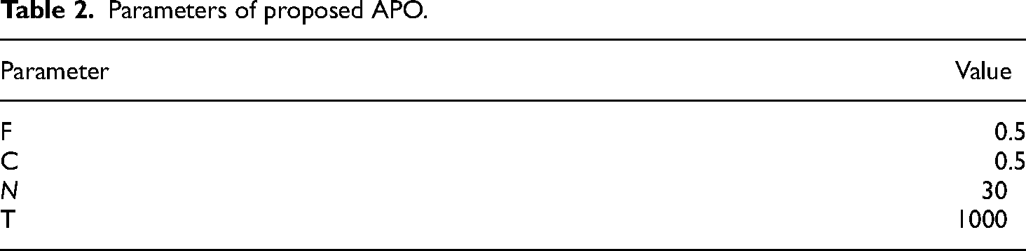
The numerical values of used parameters of APO in this study are illustrated in Table 2.

Table 2.

Parameters of proposed APO.

Parameter	Value
F	0.5
C	0.5
$N$	30
T	1000

Thorough description for the suggested FLC

FLC is a sophisticated methodology employed for the purpose of ascertaining and tracking the maximum output power of a solar system. Fuzzy set theory is utilized as an alternative to employing a precise mathematical model. The operational mechanisms of a Mamdani-type fuzzy controller are found upon the configuration seen in Figure 10.⁶⁰ Procedures of FLC is generally detailed as follows:

Fuzzification phase: this phase involves determining the degrees of membership to the related fuzzy sets predefined in the fuzzy system's database for each real input value. The conversion of the actual inputs into symbolic data that the inference process can use is done by this block.

Inference phase: This phase is the calculating the truth degree of rules of the system in combining the output to each of these rules.

Defuzzification phase: the defuzzification mechanism is to replace the output sets that produced by the inference stage by a single real value. MF inputs and outputs of FLC can take different shapes and types, they can be triangles, trapezoidal, or Gaussian.

Figure 10.

Block diagram representation of FLC.

From the figure above, fuzzy logic has two inputs. The input $E (k)$ indicates whether the PV module's operating point is on the left (Region 1, where $E (k)$ is positive), right (Region 3, where E(k) is negative), or at maximum power (Region 2, where $E (k)$ is zeros) of the $P_{P V}$ - $V_{P V}$ curve. The input $d E (k)$ determines the duty cycle change ( $d D (k)$ ) to be increased or decreased. Figure 11 illustrates the variables of the FLC's MFs (X1, X2,…, X15) that are undergone through the optimization process.

Figure 11.

Optimization procedure of the FLC's MFs.

Figure 11's MFs are derived from five levels of linguistic variables: negative large (NL), negative small (NS), zero (Z), positive small (PS), and positive large (PL). Usually, five language variables are sufficient for efficient control and trajectory tracking. Table 3 depicts the rule base that has been utilized as knowledge base for the FLC.⁵¹ The endpoints of MFs, denoted as X1 to X15, are optimized using various strategies to get their optimal values. Simply said, the optimization algorithm's purpose is to effectively handle these values. In addition, the scaling factors (G1, G2, and G3) have also been subjected to the optimization procedure in order to ascertain the appropriate duty cycle (dD) for the switching device of the boost converter. This enables the system to track the MPP corresponding to different climatic conditions.

Table 3.

The suggested rule base for FLC.

	dE
E	NL	NS	ZE	PS	PL
NL	Z	Z	PL	PL	PL
NS	Z	Z	PS	PS	PS
Z	PS	Z	Z	Z	NS
PS	NS	NS	NS	Z	Z
PL	NL	NL	NL	Z	Z

The FLC under consideration is comprised of two inputs, namely the error ( $E (k)$ ) and the rate of change of error ( $d E (k)$ ), and a solitary output, which corresponds to the rate of change of the output duty cycle ( $d D (k)$ ). The below equations can be utilized to represent the FLC's inputs and outputs:

E (k) = \frac{P_{P V} (k) - P_{P V} (k - 1)}{V_{P V} (k) - V_{P V} (k - 1)}

(28)

d E (k) = E (k) - E (k - 1)

(29)where

P_{P V} (k)

and

V_{P V} (k)

represent the output power and voltage of the PV system at sample k, respectively. However,

P_{P V} (k - 1)

and

V_{P V} (k - 1)

are the output power and voltage at sample (

k - 1)

. Thus, the error is defined as the deviation in output power between consecutive samples relative to the deviation in output voltage between the same samples.

The duty cycle utilized for driving the Insulated Gate Bipolar Transistor (IGBT) in the boost converter may be mathematically represented as follows:

D (k) = G_{3} \times d D_{N} (k) + D (k - 1)

(30)The duty cycle value at the current sample,

D (k)

, is the sum of the duty cycle value at the previous sample,

D (k - 1)

, and the rate of change in the output duty cycle, (

d D (k)

), which is the output of the FLC.

The following two sub-sections state the shapes of MFs and gain factor based on classical FLC (i.e. without any optimization), and then illustrate them when using different optimization algorithms.

FLC-unoptimized version

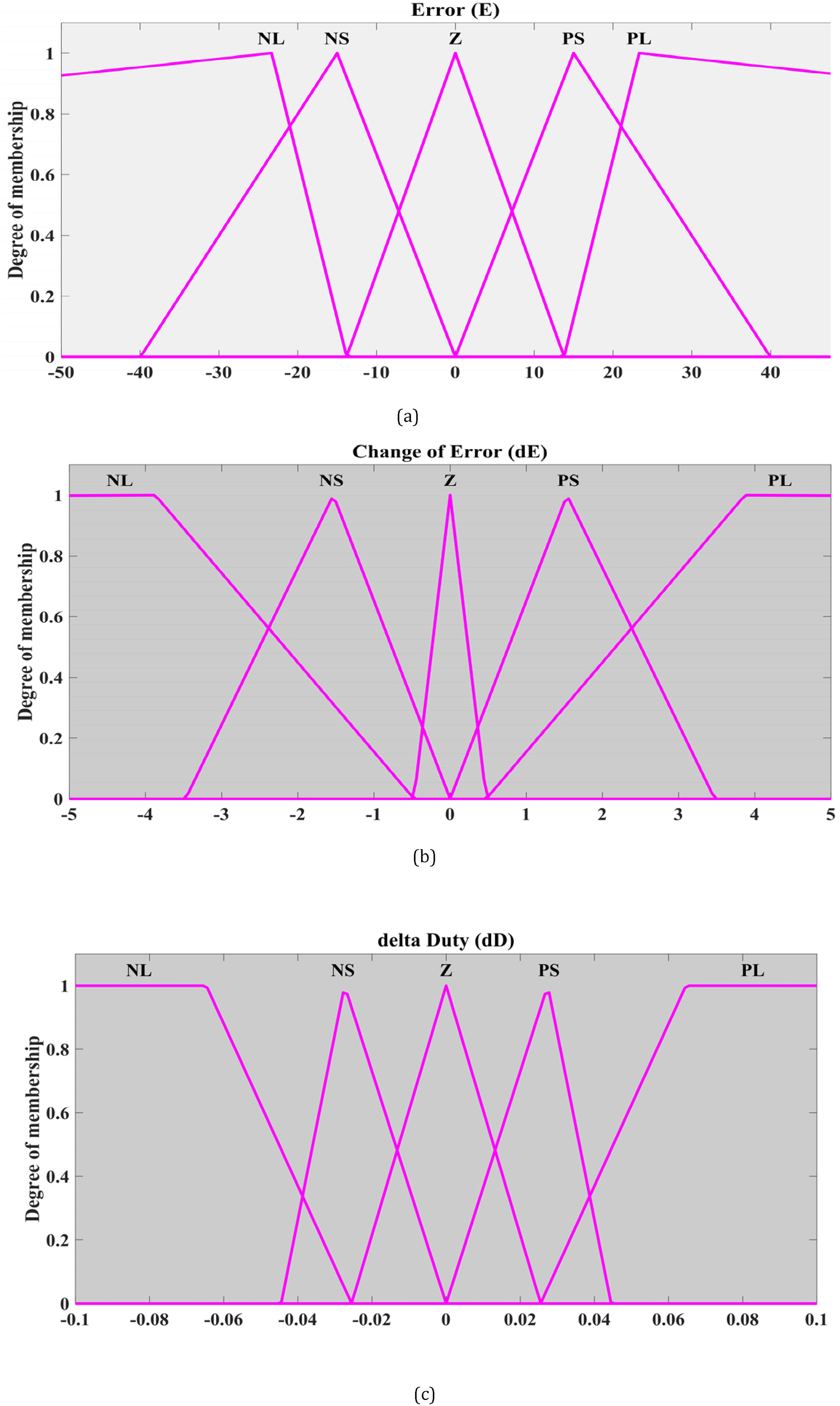
Figure 12(a) to (c) displays the unoptimized MFs of the inputs and output, with default limits (X1 to X15) set at equal intervals. The unoptimized gain factors (G1, G2, G3) are set to a default value of one for all of them.

Figure 12.

Mfs for FLC; (a) MFs for FLC's input error, (b) MFs for FLC’s input change of error and (c) MFs for FLC's output duty cycle.

FLC-optimized version

Although previous studies illustrated that FLC proved its efficiency as a MPPT, but its MFs need to be optimized to improve its performance.

In this section, different optimization algorithms are used for optimal selection of MFs of inputs and output and for the gain factors of the controller, as well. Optimization is done by PSO, GWO, and the proposed APO. In general, there are four functions used to evaluate the behavior of a control system: Integral Absolute Error (IAE), Integral Time Absolute Error (ITAE), Integral Square Error (ISE), and Integral Time Square Error (ITSE). In this study, ISE is chosen due to its benefits, such as effectively minimizing significant deviations, reducing oscillations, improving stability, and simplifying analysis and design. Therefore, the fitness function (FF) to be minimized is given by the following equation:

\min . F F = \int_{0}^{t_{s}} (E (t))^{2} \cdot d t

(31)where

t_{s}

denotes the considered time for simulation and

E (t)

denotes the deviation between the desired maximum power and the output power of the PV panel. This deviation can be mathematically derived using the following equation:

E (t) = P_{m a x} (t) - P_{P V} (t)

(32)where

P_{\max}

stands for the PV panel rated MPP and

P_{P V}

is the PV panel`s instantaneous power. System performance is evaluated in each scenario by comparing all strategies with the classical FLC case. The optimized MFs) of the inputs and output for each optimization procedure may be noticed in Figures 13–15. Additionally, the optimized gain factors are reported in Table 4.

Figure 13.

Optimal membership functions using FLC-PSO; (a) MFs for FLC’s input error, (b) MFs for FLC’s input change of error and (c) MFs for FLC's output duty cycle.

Figure 14.

Optimal membership functions using FLC-GWO; (a) MFs for FLC’s input error, (b) MFs for FLC’s input change of error and (c) MFs for FLC’s output duty cycle.

Figure 15.

Optimal membership functions using FLC-APO; (a) MFs for FLC’s input error, (b) MFs for FLC’s input change of error and (c) MFs for FLC’s output duty cycle.

Table 4.

Optimized gain factors using different optimization strategies.

Parameters	FLC-based PSO	FLC-based GWO	FLC-based APO
$G 1$	35.81	0.427	7.124
$G 2$	47.59	29.547	49.554
$G 3$	39.04	2.721	13.763

Scenarios and comprehensive analysis

This part illustrates the obtained outcomes of the PV system overall when using the FLC-based MPPT controller in four distinct versions:

Unoptimized membership functions and gain factors using classical FLC

Optimized membership functions and gain factors using FLC-based PSO.

Optimized membership functions and gain factors using FLC-based GWO.

Optimized membership functions and gain factors using FLC-based APO.

According to the EN50530 standards for testing MPPT in PV systems, the standard provides a benchmarking framework to assess the tracking efficiency and response of the MPPT in terms of the percentage of the PV system's rated power. Similar tests will be conducted in the following cases. EN50530 specifies that MPPTs must undergo two main types of tests: static and dynamic. The static test is performed under steady-state conditions of both temperature and irradiance. In contrast, dynamic tests involve variations in temperature, irradiance, or both, either gradually or rapidly. In the following subsections, situation (I) can be considered as a static test of the MPPT under stable climatic conditions, while situations (II) to (VII) can be considered as dynamic tests with varying climatic conditions either gradually or rapidly.

Hence, we have the following testing situations:

Situation I: STC at constant irradiance of 1000 W/m² and temperature of 25 °C.

Situation II: Sudden change of temperature at a constant irradiance of 1000 W/m².

Situation III: Sudden change of irradiance at a constant temperature of 25 °C.

Situation IV: Sudden change of both the temperature and irradiance together.

Situation V: Gradual change of temperature at a constant irradiance of 1000 W/m².

Situation VI: Gradual change of irradiance at a constant temperature of 25 °C.

Situation VII: Gradual change of both the temperature and irradiance together.

Therefore, the comparison between all MPPT techniques at each case are shown and explained in the subsequent figures. The evaluations are based on the tracking efficiency and oscillation levels around the steady-state MPP.

Situation I: STC at constant irradiance of 1000 W/m² and temperature of 25 °C

Under STC, Figure 16 illustrates the power profile of the PV module after it has been subjected to three different optimization strategies. This is in contrast to the classical FLC that was considered in the previous illustration. It can be seen from Figure 16 that the FLC-APO generates the lowest oscillation ratio by 0.18%, followed by the FLC-GWO with 1.07%, the FLC-PSO with 3.5%, and the classical Fuzzy with 3.7%. Based on the effectiveness of MPP tracking, the classical fuzzy algorithm is the poorest one, with a score of 98%, the FLC-PSO algorithm has a score of 98.2%, the FLC-GWO algorithm has a score of 99.4%, and the suggested FLC-APO algorithm has a score of 99.9%. Regarding the tracking time for each technique, the FLC-APO is the fastest one it takes only 12 milliseconds, followed by FLC-GWO by 18 milliseconds, FLC-PSO by 30 milliseconds, and finally 35 milliseconds for the unoptimized FLC.

Figure 16.

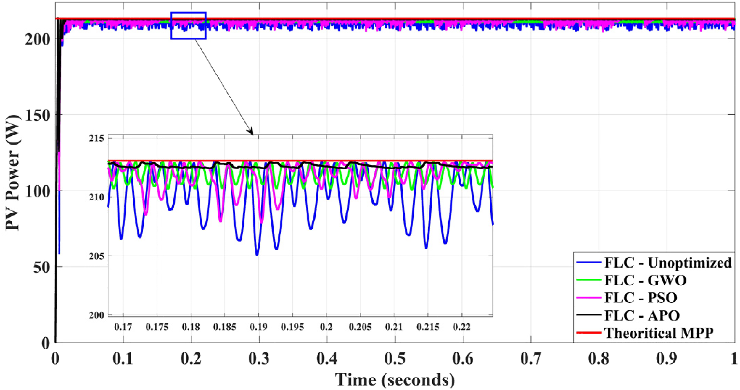
The PV module power profile considering three strategies for optimization against classical FLC under STC.

Situation II: sudden change of temperature at a constant irradiance of 1000 W/m²

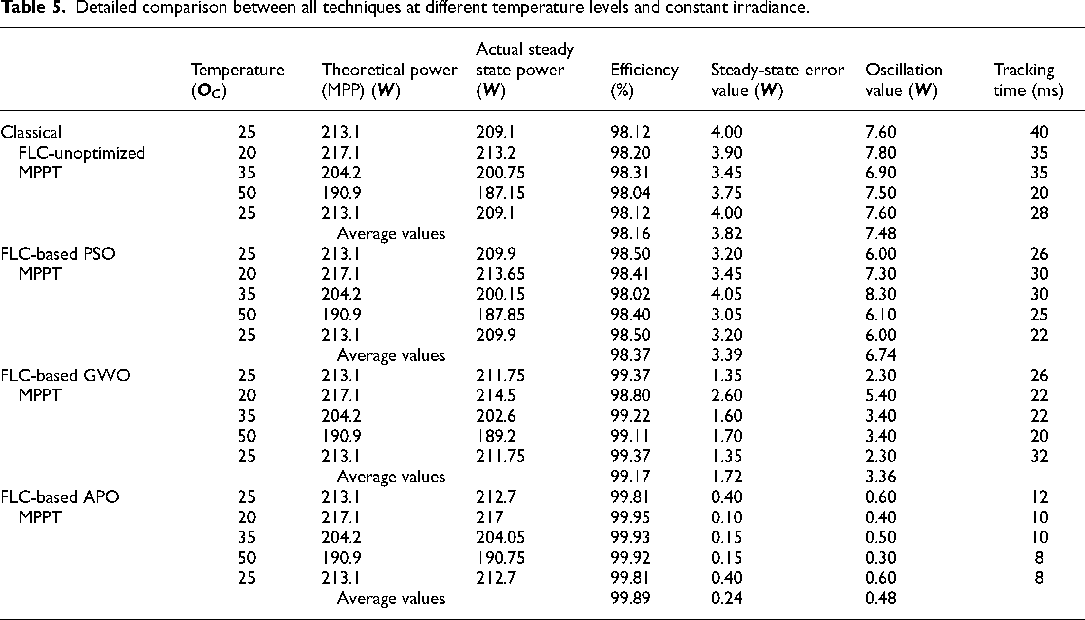
The comparison that is depicted in Figure 17 is carried out under the conditions of a constant irradiance and a rapid change in temperature. Since the levels of oscillation and efficiencies alter during the entirety of the testing period, the values of these variables are considered to be averages. As a result, the FLC-APO generates the lowest average oscillation ratio by 0.23%, followed by the FLC-GWO with 1.62%, the FLC-PSO with 3.25%, and the classical Fuzzy with 3.6%. The classical fuzzy model comes in with a score of 98.2%, while the FLC-PSO model has a score of 98.4%, the FLC-GWO model has a score of 99.2%, and the proposed FLC-APO model has a score of 99.9%. Consequently, for more illustration, a detailed numerical comparison is shown in Table 5.

Figure 17.

The PV module power profile considering three strategies for optimization against classical FLC under fast change of temperatures and constant irradiance; (a) Temperature pattern, (b) PV output power.

Table 5.

Detailed comparison between all techniques at different temperature levels and constant irradiance.

	Temperature ( $O_{C}$ )	Theoretical power (MPP) ( $W$ )	Actual steady state power ( $W$ )	Efficiency $(%)$	Steady-state error value ( $W$ )	Oscillation value ( $W$ )	Tracking time (ms)
Classical FLC-unoptimized MPPT	25	213.1	209.1	98.12	4.00	7.60	40
	20	217.1	213.2	98.20	3.90	7.80	35
	35	204.2	200.75	98.31	3.45	6.90	35
	50	190.9	187.15	98.04	3.75	7.50	20
	25	213.1	209.1	98.12	4.00	7.60	28
	Average values			98.16	3.82	7.48
FLC-based PSOMPPT	25	213.1	209.9	98.50	3.20	6.00	26
	20	217.1	213.65	98.41	3.45	7.30	30
	35	204.2	200.15	98.02	4.05	8.30	30
	50	190.9	187.85	98.40	3.05	6.10	25
	25	213.1	209.9	98.50	3.20	6.00	22
	Average values			98.37	3.39	6.74
FLC-based GWOMPPT	25	213.1	211.75	99.37	1.35	2.30	26
	20	217.1	214.5	98.80	2.60	5.40	22
	35	204.2	202.6	99.22	1.60	3.40	22
	50	190.9	189.2	99.11	1.70	3.40	20
	25	213.1	211.75	99.37	1.35	2.30	32
	Average values			99.17	1.72	3.36
FLC-based APOMPPT	25	213.1	212.7	99.81	0.40	0.60	12
	20	217.1	217	99.95	0.10	0.40	10
	35	204.2	204.05	99.93	0.15	0.50	10
	50	190.9	190.75	99.92	0.15	0.30	8
	25	213.1	212.7	99.81	0.40	0.60	8
	Average values			99.89	0.24	0.48

Situation III: sudden change of irradiance at a constant temperature of 25 °C

At a temperature of 25 °C, the temperature becomes the constant parameter, while the sun irradiation becomes the variable parameter. This happens in contrast to the prior situation. In accordance with what was mentioned before, the tracking efficiency and oscillation levels are both considered to be average values. Following the Proposed FLC-APO, which was found to be the best one by 99.8% and 0.4%, the FLC-PSO came in second with 98.6% and 3.1%, and the FLC-GWO came in third with 97.6% and 5.1%. A last point to consider is that the classical FLC situation is the worse by a margin of 96.2% and 7.9% for average oscillation and average efficiency, respectively. Figure 18 provides a visual representation of the comparison. In light of this, for further information, an illustration of a numerical comparison may be seen in Table 6. Comparisons between all considered MPPT techniques under the first three cases are summarized in Figures 19 and 20.

Figure 18.

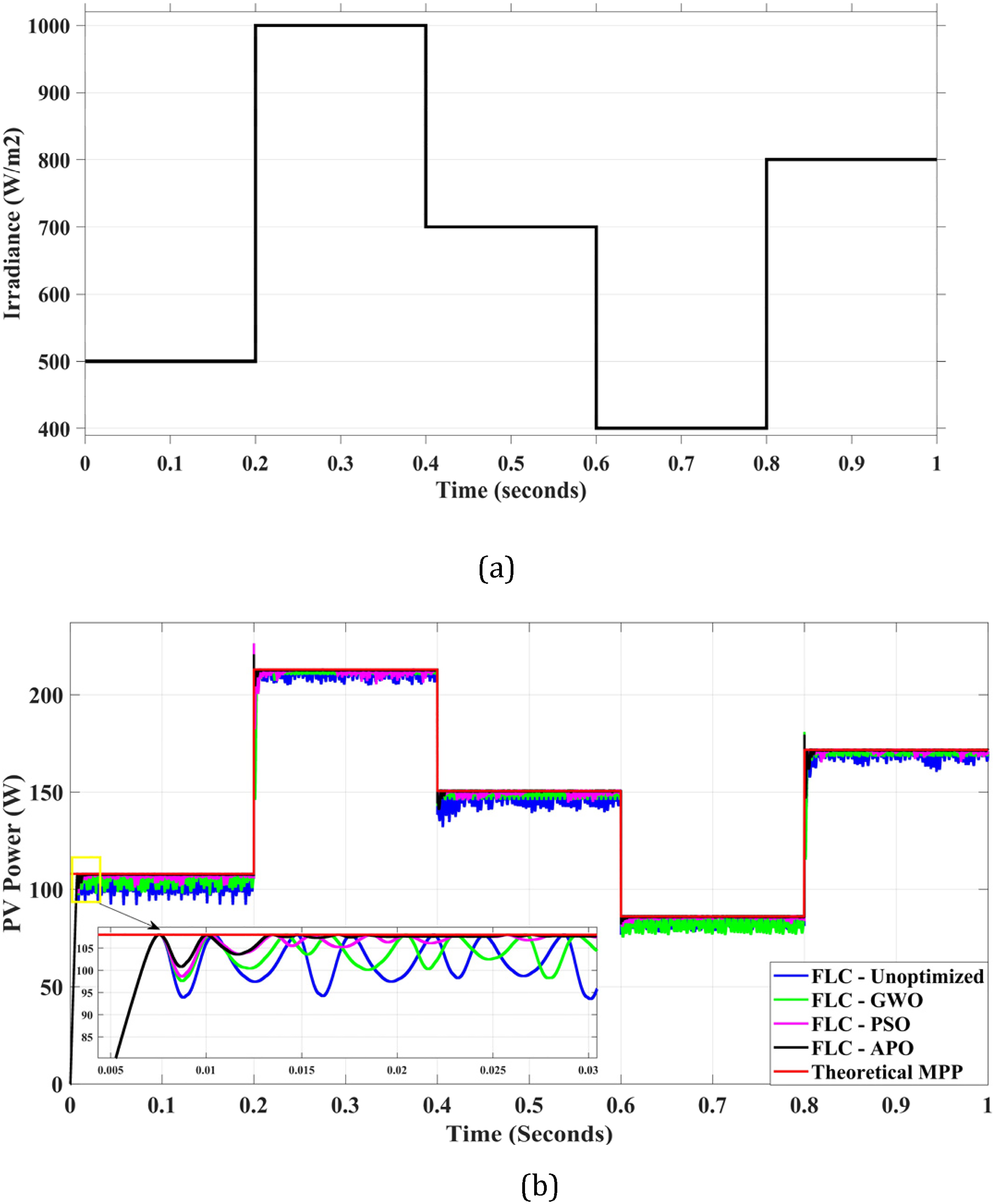
The PV module power profile considering three strategies for optimization against classical FLC under fast change of irradiance and constant temperature; (a) irradiance pattern, (b) PV output power.

Figure 19.

Comparison of average efficiency for each technique at the first three cases.

Figure 20.

Comparison of average oscillation value for each technique at the first three cases.

Table 6.

Detailed comparison between all techniques at different irradiance levels and constant temperature.

	Irradiance (w/m²)	Theoretical power (MPP) (W)	Actual steady state power (W)	Efficiency %	Steady-state error value (W)	Oscillation value (W)	Tracking Time (ms)
Classical FLC MPPT	500	108	100.2	92.8	7.8	15.4	15
	1000	213.1	209.4	98.3	3.7	7.2	25
	700	150.6	145.25	96.4	5.3	11.1	32
	400	86.1	82.45	95.8	3.7	7.7	35
	800	171.1	167.05	97.6	4.0	9.7	20
	Average values			96.2	4.9	10.2
FLC-based PSO MPPT	500	108	105	97.2	3.0	5.8	15
	1000	213.1	210.15	98.6	2.9	5.7	18
	700	150.6	148.7	98.7	1.9	4.2	25
	400	86.1	85.4	99.2	0.7	1.8	25
	800	171.1	170	99.4	1.1	3.6	20
	Average values			98.6	1.9	4.2
FLC-based GWO MPPT	500	108	103.25	95.6	4.8	9.5	15
	1000	213.1	211.8	99.4	1.3	2.4	15
	700	150.6	148.65	98.7	1.9	4.3	20
	400	86.1	81.7	94.9	4.4	9.2	25
	800	171.1	170.1	99.4	1.0	3.4	25
	Average values			97.6	2.7	5.8
FLC-based APO MPPT	500	108	107.8	99.8	0.2	0.4	15
	1000	213.1	212.7	99.8	0.4	0.6	12
	700	150.6	150.45	99.9	0.2	0.7	12
	400	86.1	85.95	99.8	0.1	0.5	10
	800	171.1	171.4	99.8	0.3	0.6	14
	Average values			99.8	0.2	0.6

Situation IV: sudden change of both the temperature and irradiance together

Here, irradiance levels and temperatures are altered in order to demonstrate the influence that these factors have on the effectiveness of MPP tracking for all of the strategies that are being investigated. Figure 21 depicts the impacts that were observed. It is demonstrated that the FLC-APO technique that was developed is capable of reaching the MPP of the system with the least amount of oscillation regardless of the variations in temperature and irradiance. It is also shown in the left zoomed area of Figure 21 that the FLC-APO model has the lowest undershoot ratio, which is 93% of its steady-state MPP. This is followed by the FLC-PSO model and the FLC-GWO model, all of which have undershoot ratios of about 91%. Nevertheless, in the right zoomed area of Figure 21, the FLC-GWO algorithm is the poorest one, accounting for 69% of its MPP. In fact, it is even worse than the classical FLC technique. As it undershoots to around 96%, FLC-APO once again demonstrated its resilience in this particular situation.

Figure 21.

The PV module power profile considering three strategies for optimization against classical FLC under fast change of both irradiance and temperature; (a) irradiance pattern, (b) temperature pattern, (c) PV output power.

There has been discussion up until this point on the impact of sudden shifts in temperature and/or solar irradiance. Furthermore, the subsequent subsections investigate the impact of altering the same parameters in a gradual way in order to demonstrate how the various MPPTs may respond to fluctuations and the degree of resilience they possess.

Situation V: gradual change of temperature at a constant irradiance of 1000 W/m²

The influence of a gradual shift in temperature while maintaining an irradiation level of 1000 W/m² is the topic of discussion in this particular instance. The reliability of FLC-APO was demonstrated in Figure 22, which demonstrates that it was able to achieve a power value that is extremely near to the theoretical one while maintaining a very low oscillation level. When the temperature drops gradually (left zoom), the tracking time of the suggested FLC-APO technique has the shortest tracking time, which is less than 1 millisecond. This is in contrast to the tracking time of the FLC-PSO technique, which is around 10 milliseconds. The other approaches, on the other hand, continue to oscillate about the steady state at a rate of roughly (5 W). On the other hand, when the temperature is gradually raised (right zoom), it is demonstrated that FLC-PSO experiences a significant undershoot that reaches 88% during the temperature change and has a significant tracking time of around 0.55 seconds. This is in contrast to the FLC-APO algorithm, which has a very low oscillation of around 0.2 W and a very tiny tracking period that exceeds 1 millisecond. On the other hand, the FLC-GWO approach continues to fluctuate by 2 W around the steady state, and the classical case is the worst one, since it oscillates by more than 5 W.

Figure 22.

The PV module power profile considering three strategies for optimization against classical FLC under slow change of temperature and constant irradiance; (a) temperature pattern, (b) PV output power.

Situation VI: gradual change of irradiance at a constant temperature

Within the context of this situation, the discussion focuses on the temperature being constant while the irradiance level gradually shifts. As was discovered, FLC-APO demonstrated its capacity to achieve the steady state rapidly with an approximate neglected error. This is in comparison to FLC-GWO, which has an error rate of 1.3%, FLC-PSO, which has a rate of 0.7%, and the classical scenario, which has a rate of 3.4%. In addition, it has been demonstrated that FLC-APO has a tracking efficiency that is greater than 99.8% when compared to other methods. In addition, when it comes to the oscillation ratio, the strategy that has been presented obviously does not exhibit any oscillation during the entirety of the simulation. Conversely, the oscillation exceeds 5% for the FLC-PSO technique and approaches 3% for the FLC-GWO technique. Figure 23 provides an illustration that highlights the comparison between all of the strategies that were investigated.

Figure 23.

The PV module power profile considering three strategies for optimization against classical FLC under slow change of irradiance and constant temperature; (a) irradiance pattern, (b) PV output power.

Situation VII: gradual change of both irradiance and temperature

In this particular scenario, there are no climatic parameters that remain constant. Temperature and irradiance level are both subject to gradual fluctuations, and the influence of these variations is being researched in order to explore the impact that these variations have on the performance of each approach that is being considered. The output power of the PV system is depicted in Figure 24, along with the performance of the three optimizations in comparison to the classical FLC system. With an ignored oscillation ratio for every aspect of parameter change, the FLC-APO that has been presented is able to track the MPP and achieve a tracking accuracy of more than 99.9%. The remaining approaches are likewise capable of reaching the MPP, but they do it with a lower efficiency that does not go beyond 98%. In addition, the oscillation ratio is greater than 3% in the vicinity of the steady state, as demonstrated in the zoomed-in portion of Figure 24.

Figure 24.

The PV module power profile considering three strategies for optimization against classical FLC under slow change of both irradiance and temperature.

Conclusions

This study entails a comprehensive analysis of how solar systems manage peak power points. The MPPT controller utilized in this study was developed through a modern optimization technique inspired by nature. The APO algorithm was employed to determine the most effective membership functions for the FLC in order to achieve the MPP of a PV solar system in various scenarios. The evaluation of the FLC-based APO MPPT model was conducted using MATLAB/Simulink and a simulated PV system, considering different climatic conditions. A study is conducted to evaluate the proposed control system, focusing on accuracy, efficiency, convergence speed, transient overshoot, and steady-state oscillation around the MPP. The proposed technique consistently exhibited a tracking efficiency of 99.8% or higher in all investigated scenarios. In addition, the oscillation ratio is the lowest compared to other MPPT approaches that were taken into consideration. The proposed method's oscillation ratio remained below 0.5%, which is lower compared to other competing strategies like FLC-based PSO, FLC-based GWO, and the classical FLC. During certain test scenarios, the application of classical Fuzzy logic led to an oscillation ratio of 10.22%. Under specific conditions, the utilization of PSO resulted in a significant decrease in the oscillation ratio, reaching 7.9%. In certain instances, the undershoot decreased from 88% using PSO to 69% when employing Grey Wolf. However, the APO that was suggested consistently maintained a ratio of at least 97%. In addition, the implementation of FLC-based APO resulted in a significant enhancement in time tracking accuracy, achieving a precision of 1 millisecond in multiple instances. The results indicate that the FLC-based APO MPPT controller outperforms the other evaluated algorithms. The suggested combination of APO and Fuzzy logic has demonstrated its effectiveness and robustness in both transient and steady-state situations. This is evident from its superior performance under standard test conditions and its ability to handle rapidly changing climatic variables such as irradiance and temperature.

While this work provides a thorough analysis of the performance of the recently proposed MPPT under various climatic conditions, it is important to acknowledge some limitations. The performance evaluation is based on simulations, whereas real-world experiments may present additional complexities and challenges. Additionally, this study focused on improving the tracking efficiency of the proposed MPPT and so, it was conducted using a single PV module, which was treated as a prototype of a PV system. However, the effects of partial shading conditions were not taken into account.

To move forward, this research suggests several directions for future work. A hardware experimental approach should be used to bridge the gap between simulation results and real-world applications. Additionally, increasing the size of the PV module to a larger PV array is essential for exploring the scalability of the system and addressing challenges such as partial shading conditions and its variations. Moreover, the proposed MPPT could be applied to other renewable energy systems, such as wind power systems, to assess its performance in a different context. Furthermore, the hybridization between APO and other optimization algorithm may be executed to evaluate its performance on the entire system, such as convergence speed tracking efficiency, and oscillation ratio.

Footnotes

Declaration of conflicting interests

The authors declared no potential conflicts of interest with respect to the research, authorship, and/or publication of this article.

Funding

The authors received no financial support for the research, authorship, and/or publication of this article.

ORCID iD

Kareem M. AboRas

References

AL-wesabi

Zhijian

Bosah

, et al. A review of Yemen’s current energy situation, challenges, strategies, and prospects for using renewable energy systems. Environ. Sci. Pollut Res 2022 Jun 21; 29: 53907–53933.

Cano

Arévalo

Jurado

. Evaluation of temporal resolution impact on power fluctuations and self-consumption for a hydrokinetic on grid system using supercapacitors. Renew Energy 2022 Jun; 193: 843–856.

Bounechba

Bouzid

Snani

, et al. Real time simulation of MPPT algorithms for PV energy system. Int J Electr Power Energy Syst 2016 Dec; 83: 67–78.

Huang

Hsu

. A performance evaluation model of a high concentration photovoltaic module with a fractional open circuit voltage-based maximum power point tracking algorithm. Comput Electr Eng 2016 Apr; 51: 331–342.

JCortajarena

Barambones

Alkorta

, et al. Sliding mode control of grid-tied single-phase inverter in a photovoltaic MPPT application. Sol Energy 2017 Oct; 155: 793–804.

Tobón

Peláez-Restrepo

Villegas-Ceballos

, et al. Maximum power point tracking of photovoltaic panels by using improved pattern search methods. Energies 2017 Sep 1; 10: 1316.

Loukriz

Haddadi

Messalti

. Simulation and experimental design of a new advanced variable step size incremental conductance MPPT algorithm for PV systems. ISA Trans 2016 May; 62: 30–38.

Alanazi

Memon

, et al. Hill climbing artificial electric field algorithm for Maximum power point tracking of photovoltaics. Front Energy Res 2022 Jul 22: 10; 10.

Fan

Cheng

, et al. Perturb and observe MPPT algorithm of photovoltaic system: a review. In: 2021 33rd Chinese Control and Decision Conference (CCDC), 2021, pp.1413–1418. IEEE.

10.

Chen

, et al. Analysis of MPPT failure and development of an augmented nonlinear controller for MPPT of photovoltaic systems under partial shading conditions. Appl Sci (Basel) 2017; 7: 95.

11.

Kwan

. High performance P&O based lock-on mechanism MPPT algorithm with smooth tracking. Sol Energy 2017; 155: 816–828.

12.

Alik

Jusoh

. Modified perturb and observe (P&O) with checking algorithm under various solar irradiation. Sol Energy 2017; 148: 128–139.

13.

Chellakhi

Said E

Younes

. Implementation of a novel MPPT tactic for PV system applications on MATLAB/Simulink and proteus-based Arduino board environments. Int J Photoenergy 2021; 2021: 200–219. https://doi.org/10.1155/2021/6657627

14.

Tey K

Mekhilef

Member

, et al. Improved differential evolution-based MPPT algorithm using SEPIC for PV systems under partial shading conditions and load variation. IEEE Trans Ind Inform 2018; 14: 4322–4333.

15.

Zaki A

Rezk

. Global MPPT based on flower pollination and differential evolution algorithms to mitigate partial shading in building integrated PV system. Sol Energy 2017; 157: 171–186.

16.

Fathi

Tousi

Galvani

. Allocation of renewable resources with radial distribution network reconfiguration using improved salp swarm algorithm. Appl Soft Comput 2023; 132: 109828.

17.

Chao

K-H

Zhang

S-W

. An maximum power point tracker of photovoltaic module arrays based on improved firefly algorithm. Sustainability 2023; 15: 8550.

18.

Benyoucef

Chouder

Kara

, et al. Artificial bee colony based algorithm for maximum power point tracking (MPPT) for PV systems operating under partial shaded conditions. Appl Soft Comput 2015; 32: 38–48. https://linkinghub.elsevier.com/retrieve/pii/S1568494615002057 .

19.

Al-Wesabi

Fang

Farh

HMH

, et al. Cuckoo search combined with PID controller for maximum power extraction of partially shaded photovoltaic system. Energies 2022; 15: 2513.

20.

Kumar

Rao

. A novel global MPP tracking of photovoltaic system based on whale optimization algorithm. Int J Renew Energy Dev 2016; 5: 225–232.

21.

Mirza

Ling

Javed

, et al. Novel MPPT techniques for photovoltaic systems under uniform irradiance and partial shading. Sol Energy 2019; 184: 628–648.

22.

Ibrahim

A-W

Shafik

Ding

, et al. PV maximum power-point tracking using modified particle swarm optimization under partial shading conditions. Chin J Electr Eng 2020; 6: 106–121.

23.

Jin

Hou

, et al. A glowworm swarm optimization-based maximum power point tracking for photovoltaic/thermal systems under non-uniform solar irradiation and temperature distribution. Energies 2017; 10: 541.

24.

Titri

Larbes

Toumi

, et al. A new MPPT controller based on the ant colony optimization algorithm for photovoltaic systems under partial shading conditions. Appl Soft Comput 2017; 58: 465–479.

25.

Dhieb

Yaich

Bouzguenda

, et al. MPPT Optimization using ant colony algorithm: solar PV applications. In: 2022 IEEE 21st International Ccnference on Sciences and Techniques of Automatic Control and Computer Engineering (STA), 2022, pp.503–507: IEEE.

26.

Fathy

. Reliable and efficient approach for mitigating the shading effect on photovoltaic module based on modified artificial bee colony algorithm. Renew Energy 2015; 81: 78–88.

27.

Atawi

Kassem

. Optimal control based on maximum power point tracking (MPPT) of an autonomous hybrid photovoltaic/storage system in micro grid applications. Energies 2017; 10: 643.

28.

Ramalu

Mohd Radzi

Mohd Zainuri

, et al. A photovoltaic-based SEPIC converter with dual-fuzzy maximum power point tracking for optimal buck and boost operations. Energies 2016; 9: 604.

29.

Hassan

Kamal

, et al. Neuro-fuzzy wavelet based adaptive MPPT algorithm for photovoltaic systems. Energies 2017; 10: 394.

30.

Nabipour

Razaz

Seifossadat

SGH

, et al. A new MPPT scheme based on a novel fuzzy approach. Renew Sustain Energy Rev 2017; 74: 1147–1169. https://linkinghub.elsevier.com/retrieve/pii/S1364032117302757 .

31.

Krishnan G

Kinattingal

Simon

, et al. MPPT In PV systems using ant colony optimisation with dwindling population. IET Renew Power Gener 2020; 14: 1105–1112.

32.

Belaidi

Haddouche

Fathi

, et al. Performance of grid-connected PV system based on SAPF for power quality improvement. In: 2016 International Renewable and Sustainable Energy Conference (IRSEC), 2016, pp.542–545: IEEE.

33.

Xia

Zhu

. Improved photovoltaic MPPT algorithm based on ant colony optimization and fuzzy logic under conditions of partial shading. IEEE Access 2024; 12: 44817–44825.

34.

Prajapati

Fernandez

. Performance evaluation of membership function on fuzzy logic model for solar PV array. In: 2020 IEEE International Conference on Computing, Power and Communication Technologies (GUCON), 2020, pp.609–613: IEEE.

35.

Messalti

Harrag

Loukriz

. A new variable step size neural networks MPPT controller: review, simulation and hardware implementation. Renew Sustain Energy Rev 2017; 68: 221–233.

36.

Dounis

Kofinas

Papadakis

, et al. A direct adaptive neural control for maximum power point tracking of photovoltaic system. Sol Energy 2015; 115: 145–165. https://linkinghub.elsevier.com/retrieve/pii/S0038092X15000626 .

37.

Villegas-Mier

Rodriguez-Resendiz

Álvarez-Alvarado

, et al. Artificial neural networks in MPPT algorithms for optimization of photovoltaic power systems: a review. Micromachines (Basel) 2021; 12: 1260.

38.

Kamal

Azar

Elbasuony

, et al. PSO-based adaptive perturb and observe MPPT technique for photovoltaic systems. In: Advances in intelligent systems and computing. Cham: Springer International Publishing, 2020. p. 125–135.

39.

Ibrahim

Ang

Dani

, et al. Optimizing step-size of perturb & observe and incremental conductance MPPT techniques using PSO for grid-tied PV system. IEEE Access 2023; 11: 13079–13090.

40.

Foster

McCray

McWhorter

. A hybrid particle swarm optimization algorithm for maximum power point tracking of solar photovoltaic systems. 2017 [cited 2025 Feb 6]. https://libjournals.unca.edu/ncur/wp-content/uploads/2021/03/2423-Nicholas-FINAL.pdf

41.

Kermadi

Salam

Ahmed

, et al. An effective hybrid maximum power point tracker of photovoltaic arrays for complex partial shading conditions. IEEE Trans Ind Electron 2019; 66: 6990–7000.

42.

Hanafiah

Ayad

Hehn

, et al. A hybrid MPPT for quasi-Z-source inverters in PV applications under partial shading condition. In: 2017 11th IEEE International Conference on Compatibility, Power Electronics and Power Engineering (CPE-POWERENG). 2017. IEEE.

43.

Avila

Pozo

, et al. Improved particle swarm optimization based MPPT for PV systems under Partial Shading Conditions. In: 2017 IEEE Southern Power Electronics Conference (SPEC), 2017. IEEE.

44.

Ram

Pillai

Rajasekar

, et al. Detection and identification of global maximum power point operation in solar PV applications using a hybrid ELPSO-P&O tracking technique. IEEE J Emerg Sel Top Power Electron 2020; 8: 1361–1374.

45.

Basiński

Ufnalski

Grzesiak

. Hybrid MPPT algorithm for PV systems under partially shaded conditions using a stochastic evolutionary search and a deterministic hill climbing. Power Electron Drive 2017; 2: 49–59. http://dx.doi.org/10.5277/PED170212

46.

Kermadi

Berkouk

. A hybrid PSO-PI based maximum power point tracking algorithm using adaptive sampling time strategy. In: 2015 4th International Conference on Electrical Engineering (ICEE), 2015, pp.1–6. IEEE.

47.

Mohanty

Subudhi

Ray

. A grey wolf-assisted perturb & observe MPPT algorithm for a PV system. IEEE Trans Energy Convers 2017; 32: 340–347. https://ieeexplore.ieee.org/document/7762891 .

48.

Farayola

Hasan

Ali

. Efficient photovoltaic mppt system using coarse gaussian support vector machine and artificial neural network techniques. Int J Innov Comput Inf Control 2018; 14: 323. http://dx.doi.org/10.24507/ijicic.14.01.323

49.

Yaouba

Welba

Bernard

, , et al. An experimental and case study on the evaluation of the partial shading impact on PV module performance operating under the Sudano-Sahelian climate of Cameroon. Front Energy Res 2022; 10: 13. http://dx.doi.org/10.3389/fenrg.2022.924285

50.

Khelifi

Guermoui

Rabehi

, et al. Short-term PV power forecasting using a hybrid TVF-EMD-ELM strategy. Int Trans Electr Energy Syst 2023; 2023: 1–14.

51.

EL-Banna

Hammad

Megahed

, et al. On-grid optimal MPPT for fine-tuned inverter based PV system using golf optimizer considering partial shading effect. Alex Eng J 2024; 103: 180–196.

52.

Katche

Makokha

Zachary

, et al. A comprehensive review of maximum power point tracking (MPPT) techniques used in solar PV systems. Energies 2023; 16: 2206.

53.

Kerid

Bounnah

. Modeling and parameter estimation of solar photovoltaic based MPPT control using EKF to maximize efficiency. Bull Electr Eng Inform 2022; 11: 2491–2499.

54.

Burnham

Johnson

, et al. Migratory movements of Atlantic puffins fratercula arctica Neumann from high Arctic Greenland. PLoS One 2021; 16: e0252055.

55.

Wang

W-C

Tian

W-C

D-M

, et al. Arctic Puffin optimization: a bio-inspired metaheuristic algorithm for solving engineering design optimization. Adv Eng Softw 2024; 195: 103694.

56.

Zhong

Meng

, et al. Opposition-based learning equilibrium optimizer with levy flight and evolutionary population dynamics for high-dimensional global optimization problems. Expert Syst Appl 2023; 215: 119303.

57.

Liu

Ding

, et al. A modified lévy flight distribution for solving high-dimensional numerical optimization problems. Math Comput Simul 2023; 204: 376–400.

58.

Wang

Chen

Ding

, et al. A novel particle swarm optimization algorithm with lévy flight and orthogonal learning. Swarm Evol Comput 2022; 75: 101207.

59.

Wang

Ran

Wang

G-G

. Role-oriented binary grey wolf optimizer using foraging-following and lévy flight for feature selection. Appl Math Model 2024; 126: 310–326.

60.

Tamalouzt

Belkhier

Sahri

, et al. New direct reactive power control based fuzzy and modulated hysteresis method for micro-grid applications under real wind speed. Energy Sources Recovery Util Environ Eff 2022; 44: 4862–4887. https://doi.org/10.1080/15567036.2022.2081741

A unique novel-based FLC approach for enhancing MPPT operation of solar systems considering sudden/gradual variation in weather conditions

Abstract

Keywords

Introduction

Background and literature

Research contribution highlights

Problem statement

Standalone PV system description

The mathematical modeling of solar system

The mathematical modeling of the boost converter

Detailed description of APO

Nature inspiration

Population matrix initialization

Exploration phase (aerial flight)

Exploitation (underwater foraging)

Factor b flexibility

Influence of parameters on performance

Algorithm complexity

Thorough description for the suggested FLC

FLC-unoptimized version

FLC-optimized version

Scenarios and comprehensive analysis

Situation I: STC at constant irradiance of 1000 W/m2 and temperature of 25 °C

Situation II: sudden change of temperature at a constant irradiance of 1000 W/m2

Situation III: sudden change of irradiance at a constant temperature of 25 °C

Situation IV: sudden change of both the temperature and irradiance together

Situation V: gradual change of temperature at a constant irradiance of 1000 W/m2

Situation VI: gradual change of irradiance at a constant temperature

Situation VII: gradual change of both irradiance and temperature

Conclusions

Footnotes

Declaration of conflicting interests

Funding

ORCID iD

References

Situation I: STC at constant irradiance of 1000 W/m² and temperature of 25 °C

Situation II: sudden change of temperature at a constant irradiance of 1000 W/m²

Situation V: gradual change of temperature at a constant irradiance of 1000 W/m²