Sage Journals: Discover world-class research

Abstract

Spatiotemporal (ST) graph modeling has garnered increasing attention recently. Most existing methods rely on a predefined graph structure or construct a single learnable graph throughout training. However, it is challenging to use a predefined graph structure to capture dynamic ST changes effectively due to evolving node relationships over time. Furthermore, these methods typically utilize only the original data, neglecting external temporal factors. Therefore, we put forward a novel time-varying graph convolutional network model that integrates external factors for multifeature ST series prediction. Firstly, we construct a time-varying adjacency matrix using attention to capture dynamic spatial relationships among nodes. The graph structure adapts over time during training, validation, and testing phases. Then, we model temporal dependence by dilated causal convolution, leveraging gated activation unit and residual connection. Notably, the prediction accuracy is enhanced through the incorporation of embedding absolute time and the fusion of multifeature. This model has been applied to three real-world multifeature datasets, achieving state-of-the-art performance in all cases. Experiments show that the method has high accuracy and robustness when applied to multifeature and multivariate ST series problems.

Keywords

Time-varying graph convolutional networks multivariate multifeature spatiotemporal series prediction

Introduction

Spatiotemporal (ST) series data typically involves temporal changes and spatial associations, and is used widely in various applications, such as environmental monitoring,¹ traffic analysis,^2,3 power system state forecasting,⁴ wind speed prediction,⁵ and solar energy generation.⁶ With the rapid development of sensor networks and mass storage technologies, the volume of collected ST series data has surged in recent years. Predicting ST series can aid in understanding trends in temporal and spatial changes, as well as interactions between different locations. This capability is crucial for forecasting future trends, devising effective management strategies to conserve resources, mitigate risks, enhance efficiency, and advance development across multiple domains.

Traditional statistical parameter models,^7–9 such as the vector auto regressive (VAR) model and hidden Markov model, excel in learning temporal features. However, they face challenges in capturing complex spatial dependencies in multivariate time series. Machine learning (ML) methods like the k-nearest neighbor (KNN) approach can handle a larger amount of data, but the prediction results are affected by the type of manual feature extractions. Recently, deep learning (DL) methods, such as recurrent neural networks (RNNs) and convolutional neural networks (CNNs),^10,11 have received significant attention from the academic community. While these models effectively learn temporal or spatial dependencies, they are typically suited for grid data, whereas practical data often involve graph structures, like social networks and urban road networks. These above-mentioned methods are less suitable for graph data, however, graph neural networks (GNNs) are adept at leveraging relationships between nodes and edges in graph structures, making them advantageous for handling non-Euclidean data. Nevertheless, GNNs currently face challenges in ST series prediction. Classical graphs are static and undirected, potentially limiting their ability to capture dynamic spatial dependencies (Figure 1(a)). Therefore, constructing dynamic graphs (Figure 1(b)) is essential to capture evolving relationships over time. Moreover, the states of variables are influenced by numerous features (Figure 2), underscoring the importance of fusing multiple variables to enhance predictive accuracy. Recently, some studies have shown that the adaptive graph achieves better results than those with static graph alone. Wu et al.¹² introduced a GNN-based model for multivariate time series, pioneering the use of learnable graph structures. To better capture ST correlations, some researchers have integrated multiple ST fusion modules to extract correlations across different time periods.¹³ Also, dynamic adaptive graphs^14,15 have been developed to learn evolving ST dependencies. Despite significant progress in ST prediction, these methods still face limitations, such as the inability to capture changing spatial relationships between nodes with only one learnable graph throughout training, insufficient integration of multiple features, or overlooking the impact of temporal patterns on ST prediction.

Figure 1.

Example of a time-varying graph in a network. Take the traffic network as an example, nodes A, B, C, D, and E represent different districts. (a) Depicts a static graph constructed based on fixed connection relationships. (b) Illustrates a dynamic graph influenced by real-time traffic data, where node interactions vary over time.

Figure 2.

Multifeature fusion at different time points. The Figure illustrates how a future feature $t \in [4, 7]$ can be influenced and predicted by three preceding features (Features 1, 2, and 3) when $t \in [0, 3]$ .

The goal of this paper is to design a time-varying graph convolution network (TVGCN) to address the aforementioned issues, supporting multifeature information fusion, and dynamically capturing the correlations between variables. To achieve this goal, we use GCN, attention and dilated causal convolution (DCCN) and other techniques. Our proposed model shows state-of-art performance on three public datasets. The contributions of this article are outlined as follows:

We propose a novel TVGCN architecture for multifeature and multivariable ST series prediction. This architecture incorporates a time-varying attention mechanism to dynamically capture spatial relationship, and uses DCCN to model time-dependent relationship, and achieves multifeature fusion through convolutional neural networks. The TVGCN effectively learns dynamic spatial and temporal dependencies among multivariate and multifeature data.

We employ a time embedding method to capture temporal patterns in practical applications, thereby enhancing prediction accuracy.

The TVGCN model generates dynamic graphs that evolve with the ST series across all stages, including training, validation, and testing.

Extensive experiments conducted on three real-world datasets demonstrate that our method can achieve state-of-art performance across different prediction horizons compared to baseline methods.

Related work

ST series prediction

Researchers have made significant strides in ST series forecasting. Initially, linear models^16,17 were employed for time series modeling, but their prediction accuracy varied widely due to data fluctuations. Subsequently, traditional ML methods like KNN⁷ and SVM⁸ were utilized, but their applicability and flexibility were hindered by intricate feature engineering.¹⁸ In recent years, DL models have demonstrated superior prediction accuracy in forecasting ST series.¹⁹ One prominent DL model, DeepAR,²⁰ pioneered the use of RNNs for time series problems. However, during prediction, it adopts the predicted value from the last time step as input rather than the actual value, potentially causing discrepancies between training and prediction stages. To address this, techniques from natural language processing have been adapted. Moreover, Rangapuram et al.²¹ proposed a deep state-space model using RNNs, where the current value depends solely on the present state, unlike DeepAR which relies on previous predictions or actual values. These models primarily focus on single-horizon forecasting. In contrast, Wen et al.²² introduced a multihorizon forecasting model named multi-Horizon quantum recurrent network, capable of predicting values multiple steps in the future. While these methods effectively extract temporal features from data, they often struggle with spatial feature extraction. Addressing this limitation, Shi et al.²³ introduced the Conv-long-short-term memory (Conv-LSTM) model, combining LSTM and CNN architectures to analyze ST features. This model notably achieved success in rainfall prediction using radar echo data. Building upon this concept, subsequent ST series methods integrating CNN structures have emerged.^24–26 Although these models can capture the dynamic ST correlations, they are only applicable to grid data.

Graph neural network

In practical applications, most data consist of graph data, and traditional DL methods often struggle to handle these effectively. Increasingly, researchers are turning to graph-based approaches for ST series prediction. To our knowledge, the STGCN²⁷ algorithm represents a pioneering effort in applying GCN to ST series problems. This model integrates time-gated convolution units and spatial convolution units to construct a fundamental ST convolution module, stacking multiple units and incorporating a residual module for enhanced performance. Inspired by the success of attention mechanisms across various domains,^28–30 researchers have begun integrating them into ST sequence prediction models. Guo et al.³¹ introduced attention into the core ST feature extraction module, creating ASTGCN. This method leverages temporal and spatial attention mechanisms to capture dynamic ST features, effectively extracting seasonal trends through multiscale temporal encoding. Despite its promising results, ASTGCN is constrained by its high computational complexity. Due to dynamic graphs’ superior ability to model evolving spatial relationships among nodes compared to static graphs, extensive research has been conducted in this area. Notable methods include MTGNN,¹² STFGNN,¹³ Graph WaveNet,¹⁴ PGCN,¹⁵ and GCN-M³² and others. Wu et al.¹² introduced MTGNN, which employs a graph learning module to analyze directional relationships among variables, utilizing multihop propagation and perceptual inflation to capture ST dependencies. Building on the adaptive adjacency matrix concept from MTGNN, Wu et al.¹⁴ proposed Graph WaveNet, incorporating dilated random convolutions to capture long-term temporal dependencies. Li et al.¹³ not only introduced dynamic spatial graphs but also employed an enhanced dynamic time warping algorithm to measure time series similarity, thereby constructing dynamic temporal graphs and integrating ST fusion. These models not only address static node connections but also propose learned and adaptive graphs based on network models. However, these studies have overlooked the impact of external temporal information on the periodicity or seasonality of spatiotemporal sequence predictions. More recently, Zuo J et al.³² proposed GCN-M, which integrates multiscale temporal embeddings and dynamic graph structures, demonstrating that incorporating external time encoding enhances the capture of ST seasonal patterns.

Dilated causal convolution

RNNs or LSTMs are typically used for sequential data processing. However, recently, more researchers have found that CNNs can effectively handle sequence data, especially due to the limitations of RNNs or LSTMs. Since sequence data inherently follows a chronological order, traditional CNNs are not initially suited for this purpose, leading to the introduction of causal convolution. Yet, causal convolution often fails to capture extensive historical context. To address this challenge, Oord et al.¹¹ proposed DCCN to enhance the receptive field of causal convolution. DCCN achieves this by introducing “holes” in convolutional kernels, enabling dense feature extraction in multilayer CNNs.²⁴ Essentially, DCCN can capture long-term temporal dependencies without significantly increasing the number of parameters.

Motivated by the aforementioned research, and taking into account the irregular grid structure and dynamic ST correlations of ST series, we propose the TVGCN method for predicting multivariate and multifeature ST series. We utilize DCCN to model the temporal dimension and GCN based on attention mechanisms to model the spatial dimension. Furthermore, we enhance prediction accuracy by integrating multiple features and encoding time into learnable vectors using a specialized method.

Problem definition

Graph definition

A graph is a data structure that represents relationships between entities, where entities are represented as nodes and their relationships as edges. The definition of graphs varies depending on the problem at hand. For instance, in the context of expressways, we can define the traffic network on the expressway as a graph $G = (V, E, A_{s t a t i c}, A_{d y n a m i c}^{t})$ , where $| V | = N$ is the set of all nodes, such as detectors on the road, and E denotes the set of all edges connecting these nodes. Each node in the traffic graph is sampled at regular time intervals, and the feature dimension of each node is F. The adjacency matrix A comprises static adjacency matrix $A_{s t a t i c}$ and dynamic adjacency matrix $A_{d y n a m i c}^{t}$ . Static adjacency matrix $A_{s t a t i c}$ means pairwise connection state and the $A_{d y n a m i c}^{t}$ is the adjacency matrix learned from feature data that varies over time.

Problem definition

Our main focus is on solving the problem of predicting ST series with multiple variables and features. For instance, we utilize historical traffic data from expressways, encompassing metrics such as traffic flow, average speed, and average occupancy rate, to forecast future traffic conditions. Given a historical ST series $[X_{1}, X_{2}, \dots, X_{T}] \in R^{N \times F \times T}$ , which has T time steps containing N nodes, each node with F features. Where $X_{t} \in R^{N \times F}$ is the graph signal on the graph $G = (V, E, A_{s t a t i c}, A_{d y n a m i c}^{t})$ , we aim to predict the entire subsequent ST sequence starting from step (T + 1). The prediction targets are the traffic flow values across all nodes, denoted as $[{\hat{Y}}_{T + 1}, {\hat{Y}}_{T + 2}, \dots, {\hat{Y}}_{T + T}]$ .

Methods

In this section, we introduce the TVGCN architecture. We then detail the methodology for constructing a time-varying graph based on attention mechanisms and the concept of time embedding. Following this, we elaborate on graph convolution operations utilizing both a static adjacency matrix and a time-varying dynamic adjacency matrix. Finally, we discuss the implementation of ST sequence prediction using DCCN in conjunction with GCN.

Model architecture

The TVGCN architecture for predicting ST series is illustrated in Figure 3. It consists of an input layer, an ST convolutional layer, and an output layer. Initially, the absolute time of the time series is encoded using the Time2Vector method, learning its representation and then integrated with the sequence features. Subsequently, the L-length sequence is segmented into T-length input samples using a sliding time window approach. These samples undergo linear transformation followed by processing through the ST convolutional layer, which comprises K (where K is 3) ST blocks. Each ST block primarily includes two components: DCCN for temporal feature extraction, and TVGCN combined with static GCN for capturing spatial dependencies among nodes. The static graph reflects physical connectivity relationships, while time-varying graphs are derived from the T-length ST series based on attention scores. The TVGCN enhances the extraction of ST relationships across multiple ST layers. The output layer aggregates results using a Relu activation function and $1 \times 1$ convolution to derive the final sequence prediction. To boost the feature extraction capability of ST information, multiple ST layers are stacked, with outputs from preceding layers feeding into subsequent ones. Residual connections are employed within each ST layer, and all layers are ultimately skip-connected to the output layer to ensure comprehensive information flow.

Figure 3.

The TVGCN architecture. Left side shows the overall structure of TVGCN, while the right side illustrates the detailed architecture of TVGCN.

When employing multiple consecutive DCCN layers, the choice of dilation coefficients primarily follows the HDC principle,³³ addressing the issue of grid-like effects. For instance, while the receptive field of dilation coefficients like [1, 2, 3] matches that of [2, 2, 2], the former optimally utilizes input information and yields superior results.

DCCN for time features extraction

The DCCN is chosen for extracting temporal features due to its benefits in parallelism, flexible receptive field adjustment, and gradient stability. Causal convolution achieves this by generating an output sequence through one-dimensional full convolution, ensuring that future predictions do not depend on future data. DCN is designed to expand the receptive field without increasing computational load. This is achieved by applying dilation, where zeros are introduced into the convolution kernel while maintaining the input unchanged. This dilation allows the network to observe longer series lengths without increasing computational complexity. After convolution and gate activation unit, the final representation of the input series $X_{t}^{(T)}$ in one sliding window T is:

H_{t} = \tanh (W_{f, k} * X_{t}^{(T)}) ⊙ σ (W_{g, k} * X_{t}^{(T)})

(1)

where

*

is the operation of convolution,

⊙

is the multiplication operation at the element level,

σ

is the activation function, k is the index of the layer, f and g represent convolution kernel and gate respectively, and

W_{f, k}

and

W_{g, k}

is learnable parameter matrix, respectively. The operation

*

of time step s in the series

X_{t}^{(T)}

is defined as:

F (s) = (X_{t}^{(T)} *_{d} f) (s) = \sum_{i = 0}^{k - 1} f (i) \cdot X_{t}^{(T)} (s - d \cdot i)

(2)

where d is the dilation factor, k is the size of the convolution kernel,

(s - d \cdot i)

indicates the past direction step,

X_{t}^{(T)}

is the input signal, and

f (i)

is the different convolution kernel. Specifically, dilation is to introduce a fixed step size between every two adjacent convolution kernels, as can be seen in Figure 3. Dilation = k means selecting an input for the next layer every k step in the current layer. When d is set to be 1, it is simplified to ordinary convolution. Additionally, the skip and residual connections are adopted into the model to keep the network stable and converging rapidly.

TVGCN for spatial features extraction

Time-varying graph construction with attention

Taking traffic flow on roads as an example, the correlation between traffic conditions at two locations dynamically changes due to various factors such as road structure, surrounding environment, weather fluctuations, and unforeseen incidents. Consequently, the mutual influence of different traffic states across locations also varies over time, illustrated in Figure 4. For instance, the interaction between a residence and a fast-food cafe might be significant in the morning but minimal in the evening. Relying solely on physical connections makes it challenging to learn spatially dynamic impacts. Therefore, to fully leverage the dynamic dependencies among nodes, we propose a dynamic adjacency matrix based on attention, which adaptively captures the evolving correlations driven by node data features:

A_{d y n a m i c}^{t} = s o f t m a x (σ ((X_{t}^{(T)} W_{1}) W_{2} {(W_{3} X_{t}^{(T)})}^{T} + b))

(3)

where

X_{t}^{(T)} \in R^{N \times F \times T}

refers to the input data divided by a sliding window,

b \in R^{N \times N}

W_{1} \in R^{T \times 1}

W_{2} \in R^{F \times T}

, and

W_{3} \in R^{F \times 1}

are all learnable parameter matrices, and

σ

is the activation function. After normalization by softmax,

A_{d y n a m i c}^{t} \in R^{N \times N}

is obtained and each value of

A_{d y n a m i c}^{t}

represents the correlation coefficient between two nodes at t. As shown in equation 3, the

A_{d y n a m i c}^{t}

changes dynamically with the change of input

X_{t}^{(T)}

and is driven by real-time traffic data. Equation 3 can be explained according to the attention method in the literature.²⁸ More importantly, it can emphasize the directionality of dynamic adjacency matrix. In the process of learning the time-varying adjacency matrix mentioned above, multihead attention method can enhance the model's expressive ability when handling high-dimensional features.

Figure 4.

Different spatial attention at different times. The darker line between nodes means greater attention.

Traffic data are physically associated with the road network. Suppose different locations on the roads as nodes, and the relationship between two nodes is determined by the connectivity between roads. Therefore, it is necessary to build the static adjacency matrix by the physical connection relationship on the road. As a result, in addition to the learnable adaptive adjacency matrix $A_{i, j}^{t}$ , a common static adjacency matrix $A_{s t a t i c}$ is constructed according to the physically connected relationship. Take the expressway for example, if two detectors in highways i and j are connected, the values of the corresponding adjacency matrices $A_{i, j}$ and $A_{j, i}$ are both 1, otherwise 0, as can be seen in equation 4, where $v_{i}$ denotes the node i in ST graph.

A_{s t a t i c} = A_{i, j} = {\begin{matrix} 1, if v_{i} and v_{j} are connected \\ 0, otherwise \end{matrix}

(4)

The decision to use node connections in the static adjacency matrix is primarily driven by the need to better reflect the accessibility and traffic flow, accurately capture the network's topology structure and facilitate computationally efficient modeling and analysis. When performing the GCN, we will accompany the dynamic time-varying adjacency matrix

A_{d y n a m i c}^{t}

with the static adjacency matrix

A_{s t a t i c}

to adjust the influence weights between the nodes dynamically.

Time-varying graph convolution network

The GCN primarily employs the concept of message passing, where nodes in the lower graph layer aggregate information from neighboring nodes in the upper layer to learn spatial dependencies. In our approach, this is realized through spatial domain graph convolution, where feature extraction occurs directly via convolutions between nodes and their neighbors. A multigraph is constructed to facilitate these convolution operations. Following the time-varying graph convolution, nodes can be represented as follows:

H^{(k)} = A_{s t a t i c} H^{(k - 1)} W_{k, 1} + A_{d y n a m i c}^{t} H^{(k - 1)} W_{k, 2}, k \geq 1

(5)

Z_{t} = f (X_{t}, A_{s t a t i c}, A_{d y n a m i c}^{t}) = \sum_{k = 0}^{k = K} H^{(k)}

(6)

where k denotes the layer number of GCN (default is 2),

H^{(k - 1)}

denotes the current input hidden layer state, represents the output hidden layer state of the current layer, the initial embedding matrix

H^{(k)}

is the node features, i.e.

H^{(0)} = X_{t}

, where

X_{t}

represents the input series within a time window,

A_{s t a t i c}

represents the static adjacency matrix constructed based on the inherent connections,

A_{d y n a m i c}^{t}

represents the dynamic adjacency matrix constructed using attention,

W_{k, 1}, W_{k, 2}

are parameter matrixes that are learned during training,

H^{(k)}

contains the high-level representations of all graph nodes based on initial features, and

Z_{t}

is the final learned node representation. Thomas's article³⁴ suggests that shallow GCNs often outperform deep GCNs without residual blocks based on experimental comparisons. The layers in a GCN network determine the furthest distance that node information can propagate. Deeper networks may spread node information across the entire network, potentially leading to less effective results. Thus, k is set to be 2 in the later experiment.

The schematic illustration of the proposed time-varying graph convolution can be seen in Figure 3. At each time step, the graph convolution involves two types of graphs. The left graph, depicted with black nodes at each time step, represents a static graph constructed based on physical connections. The right graph represents the time-varying graph, constructed using features that evolve over time. $X_{t i}$ means $[x_{t i}, x_{t i + 1}, \dots, x_{t i + T - 1}]$ , namely, where $x_{t i} \in R^{N \times F}$ , namely, N nodes, F features, and T time steps. $X_{t i}$ changes over time via a sliding window, the graph exhibits time-varying characteristics. Layers 1 and 2 in the GCN mean two-layer graph convolution, corresponding to $H^{(1)}$ and $H^{(2)}$ in equation 6, respectively. $Z_{t i}$ means the output of graph convolution at each time step.

External time embedding

Some ST data are influenced by absolute time factors, such as traffic conditions in different locations varying with the time of day, day of the week, and whether it's a weekday or weekend, all of which significantly impact prediction accuracy. Therefore, absolute time features including year, month, day, and hour can be embedded as vectors and incorporated into the network during training.

Time vectors can be embedded manually or through a functional method. Manual embedding requires specific rules tailored to different time series scenarios, with varying impacts on the same dataset. Hence, the paper adopts a general functional embedding method where time is embedded into vectors within the network for joint training and testing. In this study, Time2Vector³⁴ is employed for time embedding, inspired by positional encoding.²⁸ Unlike multiscale approaches used in other studies^31,32 for extracting seasonal patterns, our method embeds time as vectors to provide a universal representation. Additionally, we use sine functions, and a linear term to separately capture periodic and nonperiodic trends in the data. This approach is straightforward to implement, avoiding the complexity of scale selection and adjustment, thus enhancing generality and facilitating integration into various model architectures. Moreover, this method demonstrates time scaling invariance (as confirmed in Kazemi et al.³⁴). The specific formula is as follows:

t 2 v (τ) [i] = {\begin{matrix} ω_{i} τ + φ_{i}, i = 0 \\ F (ω_{i} τ + φ_{i}), 0 < i < k \end{matrix} .

(7)

where

τ

is the feature of the original time series and

F

denotes the activation function. To enable the algorithm to capture periodicity, the

F

is implemented as sin() function.

ω_{i}

and

φ_{i}

are learnable parameters. k is the output dimension of time embedding (it can be an integer multiple of the input original time series feature dimension, and 24 is selected in the Toy experiment after comparative verification). The linear term (when i = 0) represents the nonperiodic process of time, capturing nonperiodic patterns in time input.

F (ω_{i} τ + φ_{i})

fits the periodic patterns within the sequence data. Time2Vector primarily encodes absolute time using learned wavelength and offset parameters.

Here is an example of time embedding, which provides further insight into equation 7 (further information are available in the source code on Github),

Input: The initialized TVGCN network, the node number N, batch size B, the size of the time window T, to maintain time synchronization among all nodes, absolute time is first extended according to node dimensions, and then extracted from the expanded dataset. Assuming absolute time includes four items: year, month, day, and hour, then the extracted absolute time is $X_{t i m e} \in R^{B \times T \times N \times 4}$ . Assuming a time embedding dimension of 24, it can learn six periodic or nonperiodic features. The learnable parameters in time embedding $W \in R^{4 \times 6}$ , bias $b \in R^{1 \times 6}$ .

Normalize $X_{t i m e}$ according to the last dimension to get $X_{t i m e_n e w}$ .

Create a tensor and fill the diagonal of the last two dimensions with the last dimension of $X_{t i m e_n e w}$ , resulting in new tensor $X_{t i m e_n e w} \in R^{B \times T \times 4 \times 4}$ , which is the implementation of the function torch.diag_embed().

Calculate $X_{t i m e_n e w} = X_{t i m e_n e w} W + b$ to obtain a new tensor $X_{t i m e_n e w} \in R^{B \times T \times 4 \times 6}$ , and split $X_{t i m e_n e w}$ into two blocks, $X_{t i m e_0}$ and $X_{t i m e_r e m a i n}$ , along the last dimension with sizes 1 and 5 respectively.

Compute $\sin (X_{t i m e_r e m a i n})$ .

Concatenate $X_{t i m e_0}$ and $\sin (X_{t i m e_{r e m a i n}})$ along the last dimension to obtain the time embedding output $X_{t i m e_e m b} \in R^{B \times T \times 24}$ .

Concatenate $X_{t i m e_e m b}$ and other features to form the final input of the TVGCN network for training.

Experiment

Our experimental verification is to answer the following questions:

Is our model competitive with other classical ST series prediction models?

Is our model competitive with the current advanced graph-based models?

Is our model stable across different time windows?

Does our model improve accuracy through the integration of time data and multiple features?

Is our model progressive with dynamic adjacency matrix constructed in the testing phase?

Our model is verified on three datasets, including a Toy dataset³⁴ and two multifeature and multivariables highway datasets, which is called PEMS04 and PEMS08 from California.³⁵ The key information of the three datasets is provided in Table 1. In addition to the ablation experiment of our model, we also compare it against the classical methods and GNN literature, including the aforementioned representative MTGNN model, a standard encoding and decoding LSTM model, and the basic autoregressive VAR model. All experimental results are averaged over at least five runs to ensure robustness. To maintain fairness, all models adopt the same training loop, datasets and evaluation process.

Table 1.

Datasets summary.

Datasets	Variables (N)	Size (timesteps)	Sample rate	Feature number
PEMS04	307	16,992	5 min	3
PEMS08	170	17,856	5 min	3
Toy Dataset	20	2000	1 day	1

Experimental setup

We use three evaluation metrics, including mean absolute error (MAE), root mean squared error (RMSE) and mean absolute percentage error (MAPE).

M A E (Y, \hat{Y}) = \frac{1}{N T} \sum_{n = 1}^{N} \sum_{t - 1}^{T} | Y_{t}^{n} - {\hat{Y}}_{t}^{n} |

(8)

R M S E (Y, \hat{Y}) = \sqrt{\frac{1}{N T} \sum_{n = 1}^{N} \sum_{t - 1}^{T} {(Y_{t}^{n} - {\hat{Y}}_{t}^{n})}^{2}}

(9)

M A P E (Y, \hat{Y}) = \frac{1}{N T} \sum_{n = 1}^{N} \sum_{t - 1}^{T} \frac{Y_{t}^{n} - {\hat{Y}}_{t}^{n}}{Y_{t}^{n}}

(10)

where N represents the number of nodes, and T denotes the number of prediction time steps. For RMSE, MAE and MAPE, lower values indicate better performance. We implemented the TVGCN model with four blocks through experimental comparison. Each block includes two ST layers, with dilation convolution coefficients set to 1 and 2 respectively. To prevent gradient explosion, the gradient clip is set to be 5. The batch size is 32, the dropout is 0.3 and the learning rate is 0.001. The GCN has two layers. The kernel size for convolution is 5. In our experiments, the MAE between the ground truth and the estimator are set as the loss function, which is minimized by gradient descent. The sizes of the training and predicting windows are 6, 12, and 24 respectively. Thus, the maximum prediction horizon is 2 h for the PEMS04 and PEMS08 datasets. The datasets are split into training, validation, and testing sets with a ratio of 7:1:2 respectively. Each experiment ran for 100 epochs.

Baselines

TVGCN is our proposed method. To evaluate our models, the experimental results were compared with other baseline methods in the following:

VAR: A well-known vector auto-regressive time series analysis method.

LSTM: A special RNN model with long short-term memory.

ASTGCN³¹: A frequency domain GCN model, which introduces ST attention into the model.

MTGNN¹²: A general and typical GNN method aimed at multivariable time series data with graph learning.

STFGNN¹³: An ST fusion GNN with various ST graphs for traffic flow forecasting.

Traffic datasets

At first, we conduct experiments on two multivariable and multifeature datasets in the traffic field, that is PEMS04 and PEMS08, which are significant in GNN research. The processed data are sampled at 5 -min intervals. The system deployed over 39,000 detectors on the expressways in several large cities of California.³⁵ Our experiment focuses on three main measurements, including total traffic flow, average occupancy rate, and average speed. Firstly, the time window is set to be 12, meaning we predict the traffic flow for the next 1 h. Table 2 shows the results of the baselines and our proposed model on the two traffic datasets with the time window length being 12. The prediction targets are the traffic flow values. For these experiments, to better compare those networks with GNN model, we directly include results obtained from other literature which can be seen in Table 2 with *. From the results we can see that deep neural network models outperform the traditional VAR model on 1 -h prediction, demonstrating the limited capability of traditional statistical methods in modeling nonlinear data with complex spatial relationships. Despite the simple structure of the LSTM model, the prediction results obtained by this method are not very satisfactory compared to the ST feature learning methods like ASTGCN, MTGNN, STFGNN, and TVGCN, mainly because the plain LSTM model fails to capture complex spatial relationships. By comparison, TVGCN gets the best results in all three metrics in both two tasks compared with the current advanced models. This means that constructing time-varying graphs in both the training and testing stages is effective. It appears that with the data changing, data-driven time-varying graphs can significantly improve robustness.

Table 2.

Results comparison on PEMS datasets with a time window length of 12.

Dataset		VAR	LSTM	ASTGCN *[31]	MTGNN	STFGNN *[13]	TVGCN
PEMS04	RMSE	42.2603	36.0676	32.82	32.6647	31.88	31.2263
	MAE	28.0130	21.9764	21.80	22.2308	19.83	19.8005
PEMS08	RMSE	34.0287	34.1172	17.47	25.9933	26.22	24.01
	MAE	21.6104	20.2318	16.63	16.8284	16.64	15.2801

VAR: vector auto regressive; TVGCN: time-varying graph convolution network; MAE: mean absolute error; RMSE: root mean squared error; LSTM: long short-term memory.

To prove the stability of the TVGCN network model, we perform experiments using time windows of 6, 12 and 24 respectively. That is, the traffic conditions for half an hour, 1 h and 2 h ahead are predicted respectively. The results are shown in Table 3. It can be seen from the table that across each fixed time length, the predictive effect of the DL methods obviously exceeds that of the traditional statistic method. With the increase of the time window length, the prediction accuracy of TVGCN gradually decreases. Nevertheless, our proposed TVGCN achieves the best prediction effect across all different time windows. While MTGNN's learnable graph method also yields promising results, a graph constructed solely during the training stage fails to accurately capture the evolving spatial dependencies between series.

Table 3.

Baselines comparison with different time lengths on PEMS04 and PEMS08 datasets.

Dataset	Model	T = 6			T = 12			T = 24
		RMSE	MAE	MAPE (%)	RMSE	MAE	MAPE (%)	RMSE	MAE	MAPE (%)
PEMS04	VAR	36.386	22.9342	0.1611	42.1813	28.0032	0.1895	51.7823	36.0813	0.2623
	LSTM	35.9375	22.1747	0.1611	36.0676	21.9764	0.1562	36.3828	22.5399	0.1602
	MTGNN	32.7044	21.385	0.2155	32.6647	22.2308	0.2229	34.4871	22.3275	0.2444
	TVGCN	31.0363	19.6932	0.1331	31.2263	19.8005	0.1384	32.7721	20.8692	0.1498
PEMS08	VAR	29.2364	19.1625	0.1277	35.1087	22.6734	0.139	37.6717	24.1603	0.1795
	LSTM	31.4824	19.4559	0.1239	34.1172	20.2318	0.1272	34.3818	20.9495	0.1309
	MTGNN	23.8044	15.9775	0.1153	25.9933	16.8241	0.1171	28.4838	18.7376	0.1265
	TVGCN	23.3765	14.9708	0.0983	24.01	15.2801	0.0985	26.0777	16.3707	0.1116

VAR: vector auto regressive; TVGCN: time-varying graph convolution network; MAE: mean absolute error; RMSE: root mean squared error; MAPE: mean absolute percentage error; LSTM: long short-term memory.

Figure 5 shows the performance comparison of different methods as the prediction horizon increases, with (a) depicting results from the PEMS04 dataset and (b) detailing results from the PEMS08 dataset. As can be seen from Figure 5, prediction errors across various methods increase with longer horizons. This increase in difficulty stems from the greater length of the prediction, which poses challenges for accurate forecasting. Nevertheless, our method TVGCN consistently achieves superior prediction results across different horizons. Furthermore, methods focusing on temporal feature extraction, such as VAR and LSTM, demonstrate strong short-term prediction results. However, due to limitations in spatial dependency learning, these methods experience significantly increased prediction errors with longer horizons. In contrast, the MTGNN model, which considers both temporal and spatial relationships simultaneously, shows a slower increase in error with longer prediction lengths. Our proposed TVGCN outperforms all other methods in prediction accuracy across all horizon lengths, showcasing the efficacy of the ST prediction framework based on multifeature fusion, all-stage TVGCN, and DCCN in effectively capturing dynamic dependencies among multiple variables.

Figure 5.

Performance comparison with the increase of horizon. (a) PEMS08 and (b) PEMS04.

To validate the efficacy of the key components in our proposed model, we conducted ablation experiments on the PEMS04 and PEMS08 datasets, as shown in Table 4. Our proposed model achieves the best performance when employing GCN, dynamic adjacency matrix during in both training and testing phases, and multifeature fusion. By comparing the results in the second and third columns of the table, we can see that the time-varying adjacency matrix is significant to improve our model's performance. Additionally, multifeature fusion through convolution enhances prediction effectiveness compared to using single features alone. Furthermore, experiments indicate that excluding dynamic adjacency matrices during testing leads to poorer performance on both PEMS04 and PEMS08 datasets. Notably, our observations during experiments show that while training errors remain minimal, testing errors increase, highlighting the diminished generalization ability when the time-varying adjacency matrix is constructed solely during training. The rightmost column in Table 4 compares experiments using a standard convolutional network versus a DCCN network under identical receptive field conditions. Results demonstrate that DCCN consistently outperforms CNN, emphasizing the importance of constructing a DCCN module.

Table 4.

Ablation study of key components of TVGCN on PEMS datasets.

Methods	TVGCN	w/o GCN	w/o A _dynamic	w/o multifeature	w/o testing_ A _dynamic	w/o DCCN
PEMS04
RMSE	31.2263	38.3698	33.1845	31.4418	50.0909	33.8368
MAE	19.8005	24.9487	21.4190	19.9704	35.3714	22.3159
MAPE (%)	0.1384	0.1739	0.1563	0.1413	0.3617	0.1669
PEMS08
RMSE	24.01	30.0794	25.5233	25.0424	40.1185	26.83
MAE	15.2801	19.3325	16.4385	15.9795	28.4340	17.6382
MAPE (%)	0.0985	0.1263	0.1099	0.1051	0.3672	0.1294

TVGCN: time-varying graph convolution network; DCCN: dilated causal convolution; MAE: mean absolute error; RMSE: root mean squared error; MAPE: mean absolute percentage error.

The structure of the DL model proposed in this study is somewhat complex, so it is necessary to evaluate the computational complexity of the DL models. Table 5 shows the computational complexity of several DL methods mentioned before, including training time, validation time, testing time, and parameter count. In Table 5, GCN-CNN is a network model where DCCN is replaced by CNN. For fair comparison, the batch size of all DL models is set to 32. It can be seen that MTGNN has the highest number of parameters due to the multiple stacked modules and convolutions. Although TVGCN has a larger number of parameters due to the adjacency matrix constructed by the attention mechanism, compared to GCN-CNN, dilated causal convolution significantly reduces parameter count under the same receptive field, thus saving time and computational resources. The smaller number of entries in the PEMS08 dataset compared to PEMS04 results in a minor difference in training time. However, despite the substantial difference in training time between LSTM and TVGCN, their prediction times are comparable, indicating TVGCN's ability to quickly predict results once adequately trained. Moreover, parallel convolution operations in TVGCN facilitate faster processing of long sequences, a critical advantage for applications requiring real-time predictions.

Table 5.

Computation time for PEMS data.

Dataset	Model	Testing time	Training time	Validating time	Parameters
PEMS04	LSTM	7.9	24.98	2.97	75,692
	MTGNN	19.35	223.56	9.27	764,940
	GCN-CNN	29.94	292.71	15.12	532,600
	TVGCN	9.63	122.95	5.13	382,456
PEMS08	LSTM	4.69	18.64	1.93	62,759
	MTGNN	9.48	98.28	5.26	601,596
	GCN-CNN	15.77	160.76	7.88	467,251
	TVGCN	5.33	67.96	2.73	317,107

CNN: convolutional neural network; TVGCN: time-varying graph convolution network; LSTM: long short-term memory.

Bold indicates the least amount of time spent and underline indicates the second least.

Toy dataset

To evaluate the impact of incorporating time data on prediction accuracy, we employed a multivariate ST dataset named Toy Dataset, which includes absolute time information and draws inspiration from.³⁶ This dataset comprises sine-wave series with multiple variables exhibiting strong interdependencies. Each ith time series is defined as shown in equation 11. We utilized the Time2Vector technique³⁴ to encode absolute time into a vector format, which was then embedded as an additional feature in the network, following the methodology outlined in section External time embedding. The absolute time information, including year, month, and day, was extracted and normalized to a [0,1] range. Subsequently, this normalized time data was incorporated into the coding function described in equation 7 of section External time embedding. Finally, the time sequence was encoded into a vector of specified dimensions and integrated into the network as additional features for learning.

f (i, t) = \sin (\frac{2 π i t}{64}) + \frac{1}{D + 1} \sum_{j = 1, j \neq i}^{D} \sin (\frac{2 π j t}{64})

(11)

where D denotes the total number of time series. In our experiment, D is set to be 20.

Table 6 presents the results of various methods using time windows of 6, 12, and 24. TVGCN represents our proposed model, while TVGCN-E denotes our proposed approach incorporating additional data encoding. Across Table 6, we observe a general trend of decreased prediction accuracy as the time window increases for most methods. However, our proposed TVGCN consistently achieves optimal results at each fixed time length. Moreover, employing the Time2Vector method for encoding absolute time also contributes to enhanced prediction accuracy. This underscores the effectiveness of integrating supplementary time data into the network to improve model performance.

Table 6.

Baselines comparison with different lengths of time window on toy dataset.

Dataset	Model	T = 6		T = 12		T = 24
Toy		RMSE	MAE	RMSE	MAE	RMSE	MAE
	VAR	0.1277	0.0946	0.1970	0.1531	0.3956	0.3262
	LSTM	0.0488	0.0359	0.0503	0.0321	0.0567	0.0423
	MTGNN	0.0246	0.0183	0.0240	0.0170	0.0195	0.0145
	TVGCN	0.0170	0.0104	0.0185	0.0141	0.0189	0.0144
	TVGCN-E	0.0145	0.0099	0.0175	0.0125	0.0176	0.0125

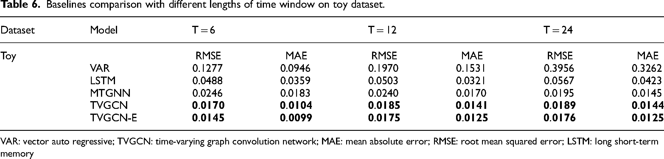
VAR: vector auto regressive; TVGCN: time-varying graph convolution network; MAE: mean absolute error; RMSE: root mean squared error; LSTM: long short-term memory

It can be seen from equation 11 that the influence coefficient between different nodes varies with the magnitude of $| \sin (\frac{2 π j t}{64}) |$ . When t is fixed, the influence coefficient of node j on node i increases with the increase of $| \sin (\frac{2 π j t}{64}) |$ . We selected four nodes with i ranging from 1 to 4, for verification. The total length of Toy dataset is 1400, 60% of which is selected for training, 10% for verification and 30% for testing. Figure 6 verifies that attention between nodes varies with time and that the magnitude of attention corresponds to the influence between nodes. It can be found from Figure 6(a) that when t ranges between 1406 and 1412, $| \sin (\frac{2 π t}{64}) | < | \sin (\frac{2 π 2 t}{64}) | < | \sin (\frac{2 π 3 t}{64}) | < | \sin (\frac{2 π 4 t}{64}) |$ , indicating that $| \sin (\frac{2 π t}{64}) |$ is the smallest, meaning that node 1 has the smallest impact on other nodes, node 2 has the larger impact on other nodes, increasing in order, and node 4 has the largest impact on other nodes. Figure 6(b) shows the adjacency matrix based on attention when t is in (1406, 1412). Notably, the attention value of the first row at this time interval is the smallest compared to other rows, indicating that node 1 has the least influence on other nodes. Conversely, node 1 is most significantly affected by other nodes due to its minimal impact, as evident in the first column of Figure 6(b), where the attention values are higher compared to other columns. As time progresses to another interval, specifically when t is in (1420, 1426), $| \sin (\frac{2 π t}{64}) |$ is relatively larger than others, suggesting that node 1 should have a greater impact on other nodes. Accordingly, in Figure 6(c), the attention values in the first row are relatively higher than in other rows. These experiments demonstrate that the time-varying adjacency matrix based on attention can effectively capture varying weight sizes with sequential data, consistent with theoretical expectations.

Figure 6.

Discovering spatial relationships from data: (a) Relationship between the constituent elements of the first four series in the toy dataset. (b) Time-varying adjacency matrix at t within the interval (1406, 1412). (c) Time-varying adjacency matrix at t within the interval (1420, 1426).

Conclusion

This paper introduces a novel ST architecture for predicting multifeature and multivariable time series. Our approach integrates a TVGCN with DCCN to capture dynamic dependencies among nodes across different time periods. Time-varying graphs are constructed using attention mechanisms between nodes in spatial dimensions. The temporal information is added to the spatial features to get good ST fusion effect. In addition, multifeature fusion through convolution is used to improve the accuracy. Experiments on three real-world datasets show that our proposed method can achieve state-of-the-art performance.

In the future, we plan to extend this ST prediction model to more complex domains such as climate and energy forecasting. While our proposed method has shown promising predictive results, there remains room for improvement in computational complexity, particularly in generating dynamic adjacency matrices. Future directions include exploring efficient techniques like matrix sparsification. Additionally, considering the heterogeneous nature and semantic properties of nodes in practical applications would further enrich the graph construction process.

Footnotes

Acknowledgments

The authors would like to express their gratitude to all those who helped them during the writing of this manuscript. The authors owe their sincere gratitude to friends and colleagues who gave them much enlightening advice and encouragement.

Author contributions

FS designed the work, obtained the dataset, performed the experiments, and drafted the work. AZ and KC edited the manuscript, performed the experiments, and organized the data. Pro H analyzed the data, revised the manuscript, and confirmed the authenticity of all the original data. All authors have read and approved the final version of the manuscript.

Data availability statement

Data availability at https://github.com/sunfeiyan666/time_series_data.git. Code availability:

Declaration of conflicting interests

The authors declared no potential conflicts of interest with respect to the research, authorship, and/or publication of this article.

Funding

The authors disclosed receipt of the following financial support for the research, authorship, and/or publication of this article: This work was supported by the National Natural Science Foundation of China, Defense Industrial Technology Development Program (Grant Nos. 72072092 and JCKY2020601B018).

ORCID iD

Wenning Hao

References

Chen

Zhu

, et al. A comprehensive analysis of environmental loading effects on vertical GPS time series in Yunnan, southwest China. Remote Sens-Basel 2022; 14: 2741.

Liu

, et al. Adaptive spatio-temporal graph neural network for traffic forecasting. Knowl-Based Syst 2022; 242: 108199.

Han

Zhao

Zhu

, et al. Spatial-temporal risk field for intelligent connected vehicle in dynamic traffic and application in trajectory planning. IEEE T Intell Transp 2023; 24: 2963–2975.

Huang

. Differential evolution-based three stage dynamic cyber-attack of cyber-physical power systems. IEEE-Asme T Mech 2022; 28: 1137–1148.

Chen

Zeng

, et al. A two-layer nonlinear combination method for short-term wind speed prediction based on ELM, ENN, and LSTM. IEEE Internet Things 2019; 6: 6997–7010.

Said

Alanazi

. AI-based solar energy forecasting for smart grid integration. Neural Comput Appl 2023; 35: 8625–8634.

Brockwell

Davis

Fienberg

. Time series: theory and methods. Berlin/Heidelberg, Germany: Springer Science & Business Media, 1991, [Google Scholar].

Ilhan

Karaahmetoglu

Balaban

, et al. Markovian RNN: an adaptive time series prediction network with hmm-based switching for nonstationary environments. IEEE T Neur Net Lear 2021; 34: 715–728.

Murphy

. Machine learning: a probabilistic perspective. Cambridge, Massachusetts: MIT press, 2012, [Google Scholar].

10.

Shahabi

, et al. Diffusion convolutional recurrent neural network: Data-driven traffic forecasting. 2017; arXiv preprint arXiv:1707.01926 .

11.

Pan

Tan

Feng

, et al. Very short-term solar generation forecasting based on LSTM with temporal attention mechanism. In: 2019 IEEE 5th international conference on computer and communications (ICCC), Chengdu, China, 6–9 December 2019, pp. 267–271.

12.

Pan

Long

, et al. Connecting the dots: multivariate time series forecasting with graph neural networks. In: Proceedings of the 26th ACM SIGKDD international conference on knowledge discovery & data mining, USA, 6–10 July 2020, pp. 753–763.

13.

Zhu

Spatial-temporal fusion graph neural networks for traffic flow forecasting. In: Proceedings of the AAAI conference on artificial intelligence, Online, 2–9 February 2021; pp. 4189–4196.

14.

Pan

Long

, et al. Graph wavenet for deep spatial-temporal graph modeling. 2019, arXiv preprint arXiv:1906.00121 .

15.

Shin

Yoon

. PGCN: progressive graph convolutional networks for spatial-temporal traffic forecasting. IEEE T Intell Transp 2024; 25: 7633–7644.

16.

Williams

Hoel

. Modeling and forecasting vehicular traffic flow as a seasonal ARIMA process: theoretical basis and empirical results. J Transp Eng-Asce 2003; 129: 664–672.

17.

Chandra

Al-Deek

. Predictions of freeway traffic speeds and volumes using vector autoregressive models. J Intell Transport S 2009; 13: 53–72.

18.

Ding

Benoit

Foggia

, et al. Neural network-based model design for short-term load forecast in distribution systems. IEEE T Power Syst 2015; 31: 72–81.

19.

Bui

KHN

Cho

. Spatial-temporal graph neural network for traffic forecasting: an overview and open research issues. Appl Intell 2022; 52: 2763–2774.

20.

Salinas

Flunkert

Gasthaus

, et al. DeepAR: probabilistic forecasting with autoregressive recurrent networks. Int J Forecasting 2020; 36: 1181–1191.

21.

Rangapuram

Seeger

Gasthaus

, et al. Deep state space models for time series forecasting. In: Advances in neural information processing systems, Montreal, Canada, 3–8 December 2018.

22.

Wen

Torkkola

Narayanaswamy

, et al. A multi-horizon quantile recurrent forecaster 2017. arXiv preprint arXiv:1711.11053 .

23.

Shi

Chen

Wang

, et al. Convolutional LSTM network: a machine learning approach for precipitation nowcasting. Advances in neural information processing systems, Montreal, Quebec, Canada, 7–12 December 2015.

24.

Bai

Kolter

Koltun

. An empirical evaluation of generic convolutional and recurrent networks for sequence modeling. 2018. arXiv preprint arXiv:1803.01271 .

25.

Wang

Zhang

, et al. Spatial-temporal feature fusion neural network for EEG-based emotion recognition. IEEE T Instrum Meas 2022; 71: 1–13.

26.

Zhao

Dai

, et al. A novel STFSA-CNN-GRU hybrid model for short-term traffic speed prediction. IEEE T Intell Transp 2022; 24: 3728–3737.

27.

Yan

Xiong

Lin

. Spatial temporal graph convolutional networks for skeleton-based action recognition. In: Proceedings of the AAAI conference on artificial intelligence, New Orleans, 2–7 February 2018, pp. 4189–4196.

28.

Vaswani

Shazeer

Parmar

, et al. Attention is all you need. In: Advances in neural information processing systems, Long Beach, CA, USA, 4–9 December, 2017.

29.

Sharma

Chen

Fard

, et al. An exploratory study on code attention in BERT. In: Proceedings of the 30th IEEE/ACM international conference on program comprehension, Pittsburgh, PA, 16–17 May 2022; pp. 437–448.

30.

Bahdanau

Cho

Bengio

Neural machine translation by jointly learning to align and translate. 2014, arxiv preprint arxiv:1409.0473.

31.

Guo

Lin

Feng

, et al. Attention based spatial-temporal graph convolutional networks for traffic flow forecasting. In: Proceedings of the AAAI conference on artificial intelligence, Hawaii, 27–31 January 2019; pp. 922–929.

32.

Zuo

Zeitouni

Taher

, et al. Graph convolutional networks for traffic forecasting with missing values. Data Min Knowl Disc 2023; 37: 913–947.

33.

Wang

Chen

Yuan

, et al. Understanding convolution for semantic segmentation. In: 2018 IEEE winter conference on applications of computer vision (WACV), Lake Tahoe, NV, 12–15 March 2018, pp. 1451–1460.

34.

Kazemi

Goel

Eghbali

, et al. Time2vec: Learning a vector representation of time. 2019, arXiv preprint arXiv:1907.05321 .

35.

Chen

Petty

Skabardonis

, et al. Freeway performance measurement system: mining loop detector data. Transport Res Rec 2001; 1748: 96–102.

36.

Shih

Sun

Lee

. Temporal pattern attention for multivariate time series forecasting. Mach Learn 2019; 108: 1421–1441.

TVGCN: Time-varying graph convolutional networks for multivariate and multifeature spatiotemporal series prediction

Abstract

Keywords

Introduction

Related work

ST series prediction

Graph neural network

Dilated causal convolution

Problem definition

Graph definition

Problem definition

Methods

Model architecture

DCCN for time features extraction

TVGCN for spatial features extraction

Time-varying graph construction with attention

Time-varying graph convolution network

External time embedding

Experiment

Experimental setup

Baselines

Traffic datasets

Toy dataset

Conclusion

Footnotes

Acknowledgments

Author contributions

Data availability statement

Declaration of conflicting interests

Funding

ORCID iD

References