Slow sound mode prediction and band structure calculation in 1D phononic crystal nanobeams using an artificial neural network

Abstract

Phononic crystals, which are artificial crystals formed by the periodic arrangement of materials with different elastic coefficients in space, can display modulated sound waves propagating within them. Similar to the natural crystals used in semiconductor research with electronic bandgaps, phononic crystals exhibit the characteristics of phononic bandgaps. A gap design can be utilized to create various resonant cavities, confining specific resonance modes within the defects of the structure. In studies on phononic crystals, phononic band structure diagrams are often used to investigate the variations in phononic bandgaps and elastic resonance modes. As the phononic band frequencies vary nonlinearly with the structural parameters, numerous calculations are required to analyze the gap or mode frequency shifts in phononic band structure diagrams. However, traditional calculation methods are time-consuming. Therefore, this study proposes the use of neural networks to replace the time-consuming calculation processes of traditional methods. Numerous band structure diagrams are initially obtained through the finite-element method and serve as the raw dataset, and a certain proportion of the data is randomly extracted from the dataset for neural network training. By treating each mode point in the band structure diagram as an independent data point, the training dataset for neural networks can be expanded from a small number to a large number of band structure diagrams. This study also introduces another network that effectively improves mode prediction accuracy by training neural networks to focus on specific modes. The proposed method effectively reduces the cost of repetitive calculations.

Introduction

Phononic crystals (PnCs) exhibit periodic distributions of elastic properties in space, which endow them with the ability to manipulate propagating elastic waves. Utilizing specific structural designs across one to three dimensions, PnCs find applications in various fields, such as sensors,^1–3 filters,^4–6 and resonators.^7–11 In 1D PnCs, a prevalent design involves simply stacking layers of two materials periodically in space, providing effective applications, such as gas and liquid sensors or absorbers.^12–14 Conversely, another complex type of 1D PnC is constructed on nanobeams, creating cavities or filters through the periodic arrangement of pillars or air holes in the nanobeam.^15–17 These types of 1D PnCs are often used to achieve acousto-optical (AO) coupling. To create cavities for both elastic and light waves simultaneously, a fishbone-shaped structure has been proposed to better generate photonic and phononic bandgaps^18,19 since the vibrations of the bone-like pillars can make the phononic bandgap more easily observed in the fishbone-like structures than for the traditional hole-type structures. Also some special modes can be produced easily for the AO coupling. To build the AO resonance cavity, the phononic characteristics of the desired structure must be investigated through the phononic band structure (PBS).

The PBS has been widely employed to investigate the behavior of elastic waves propagating within a specific PnC. The PBS reveals the characteristics of the corresponding PnC in the form of a dispersion relationship. Due to the crystal-like structure, the characteristics of PnCs are usually investigated via the reciprocal space, also known as the k-space. Therefore, each point in the PBS represents a possible wave mode existing in the corresponding reciprocal space, with the location marked on the basis of the k vector. In the following PBS figures, the x-axes are labeled from 0 to 0.5 with the unit of 2π/a, representing the reduced k vector; meanwhile, the y-axes are the eigenfrequencies of the eigenmodes. These include features such as the phononic bandgap (PBG), slow sound (SS), or other resonant elastic modes.

Multiple techniques exist for solving the PBS, including the plane-wave expansion method, finite-difference time-domain method, ²⁰ and finite-element method (FEM). ²¹ Notably, the FEM is renowned for its computational advantages, particularly when dealing with intricate structures. By imposing periodic boundary conditions on the relevant unit cell boundaries of the PnC following Bloch's theorem, the characteristics of the PnC structure can be computed using a single unit cell. Subsequently, the PBS can be derived by solving eigenvalue problems within the reduced Brillouin zone specific to the PnC.

Typically, analyses of the PBS involve varying the geometric parameters or altering the material properties. Several PBS analyses are required to illustrate the frequency shift of the elastic modes with changing parameters. By examining the relationships revealed through the PBS, the design of PnC structures can be tailored to achieve specific resonant frequencies or suitable PBG ranges. Consequently, a PBS analysis is often iterative and time-intensive. For such repetitive tasks, commonly used software can assist researchers in automating the calculations. However, because of the continuous accumulation of data during the automated calculation process, memory may be occupied, potentially increasing the required time.

Recently, ANN research has garnered increasing attention across diverse fields. The strong computational ability of ANNs has been effectively employed to analyze complex nonlinear relationships, recognize patterns, and design optical and electromagnetic devices.^22,23 In 2024, Li et al. proposed an ANN-supported structure design method. ²⁴ They used the bandgap width and some geometric parameters as the features to train the network and designed a wide-bandgap topological device. By simulating the information transmission within the biological neuron network, even the simplest configuration of a neural network consists of fully connected layers, which serve as the primary layers of the network, with computational capabilities facilitated by the activation function and the weights of each neuron. The network comprises an input layer, an output layer, and several hidden layers between the two layers. By providing the desired target for prediction and suitable features as inputs, the network begins with a randomly set group of weights and biases for the neurons and automatically adjusts these weights according to the mean square error (MSE). After sufficient training, the network obtains the best weight combinations, and the trained ANN can predict a wide array of data types.

In early studies on ANNs, the primary challenge was extracting important features from raw data or adjusting the activation function to enhance the reactivity of neurons. Currently, the software readily offers default configurations for fully connected types of ANNs, enabling straightforward adjustments to the number of neurons within the hidden layers and the number of hidden layers to facilitate the calculation functionality in the ANN.

In the previous literature, using ANNs to predict the characteristics of PnCs or even the photonic crystal structures is difficult to be achieved, due to the complexity and the non-linearity of the BS of these periodic structures. The proposed ANN may achieve the prediction by huge construction, ²⁵ or can only work on a relatively simple band structure with only a few modes, ²⁶ or it needs an extremely large amount of data for training the ANN. ²⁷ For instance, Seid et al. ²⁷ proposed a machine learning-based approach to classify the band gap properties of PnCs. The method can classify the PnC with phononic bandgaps and give the predicted bandgap center frequency and bandwidth. However, to train this prediction of ANNs, a huge number of PBSs calculated from a total of 14,112 PnCs with different geometric and physics parameters were needed as the raw data. On the other hand, Adriano et al. ²⁶ designed an ANN to compute the BSs for photonic crystals. Although the proposed ANN can work on both photonic crystals in 2D square-lattices and in 3D simple-cubic lattices, the desired BS as the training target only contains two and six photonic bands, respectively, for the 2D and 3D photonic crystals. In 2023, Caspar et al. ²⁵ demonstrated a neural network configuration to predict the BS of photonic crystal waveguides. The proposed method has high accuracy and high computation speed compared to the traditional simulation methods. However, it needs not only 100,000 band structures as the raw data, but also a stacked multilayer construction network with 500 nodes per layer.

In this study, a well-trained ANN was introduced to support conventional repetitive procedures in PBS calculations with a simple two-hidden-layer configuration. Using just a few of the PBSs calculated through the FEM simulation as the training dataset for the ANN, the remaining PBSs can be predicted using the trained ANN. By considering the frequencies of the elastic modes within the PBS as prediction targets and utilizing the geometric parameters of a 1D fishbone-like PnC structure and the reduced k vectors of the elastic modes as input data, our objective is to train the ANN to predict the PBS using as little raw data as possible while maintaining accuracy.

Materials and methods

Figure 1(a) presents a schematic of the unit cell of the 1D fishbone-like PnC. The unit cell exhibited periodic arraying in the y-direction, forming a 1D nanobeam with a period length a of 440 nm. The thickness of the nanobeam is denoted as H, and the basic width is denoted as w, and they have values of 220 and 440 nm, respectively. The fishbone-like shape was achieved by periodically drilling two semicylinders on both sides of the nanobeam in the x-direction, and the radius of the drilled hole, r, was defined as a fraction of a. To manipulate the resonant frequency of the elastic mode existing in the PnC, an additional width, dw, was defined as the wing of the fishbone between the cylinder holes.

Figure 1.

(a) Sketch of the fishbone-like nanobeam unit cell. (b) PBS of the PnC with r = 0.3a, dw = 0.5w. (c) Displacement field and (d) strain field of the SS mode marked in red in (b).

The nanobeam is made of silicon and is considered to be an anisotropic material with a density of 2320 kg/m³ and a symmetric elastic matrix defined as C₁₁= C₂₂= C₃₃=  $16.56\times {10}^{10}\mathrm{N}/{\mathrm{m}}^2$ , C₁₂= C₁₃= C₂₃=  $6.39\times {10}^{10}\mathrm{N}/{\mathrm{m}}^2$ , and C₄₄= C₅₅= C₆₆=  $7.95\times {10}^{10}\mathrm{N}/{\mathrm{m}}^2$ . The PBS was initially computed using FEM with COMSOL Multiphysics software using the Solid Mechanics model. By applying periodic boundary conditions to the unit cell boundaries in the periodic direction, the eigenmodes within the PnC can be simulated. Both dw and r were treated as variables to manipulate the resonant frequency. According to the value used in our previous works for acousto-optics coupling structures,^15,16,28 the value of dw ranged from 0 to 0.5w in increments of 0.1w and the value of r ranged from 0.1a to 0.4a in increments of 0.01a. Out of 186 sets of raw data, a specific ratio of data, with the value defined as Rd, was randomly extracted to train the ANN. The lower value of Rd represents a less requirement for raw PBS data and more calculation time can be saved.

Figure 1(b) shows the PBS corresponding to r = 0.3a and dw = 0.5w. In this PBS representation, each point denotes an elastic eigenmode at a specific reduced k vector. To increase the amount of data in the dataset further for ANN training, each eigenmode point was treated as an individual data point. Therefore, each PBS can contribute 375 data points, and the number of training data points were increased to $186\times R_d\times 375$ in total. Figure 2 depicts the configuration of the fitting ANN designed for PBS prediction using the math software MATLAB. The input layer, as illustrated in Figure 2, comprises four features as input neurons: the geometric information of the r/a and dw/w ratios, and the information extracted from the PBS, represented by k and the eigen order (EO). The information extracted from the PBS corresponds to the x- and y-coordinates of the points. The x-coordinate of the PBS represents the reduced k vector within the reduced Brillouin zone, and the y-coordinate represents the eigenfrequency of the mode points. As the eigenfrequency of the mode is the output target of the ANN, another variable is required to identify the location of the points in the y-direction. For an intuitive representation in the y-direction, the EO was chosen as the representative variable, starting from 1 for the lowest frequency at a specific reduced k vector and increasing with the number of solutions.

Figure 2.

Configuration of the ANN designed for PBS prediction.

There were two hidden layers consisting of 25 neurons each, and the activation functions were sigmoid functions. Typically, an excessive number of layers may cause overfitting, yielding low-fitting accuracy results for data that are not part of the training dataset. Concerning the number of neurons, empirical evidence suggests that a greater number enhances ANN performance but extends the training duration. Given the requirement of high accuracy in predicting the PBS, specific values for the number of hidden layers and neurons were established through numerous tests. Ultimately, the output layer comprises a single neuron representing the eigenfrequency of the mode points, serving as the training target for the ANN. The Bayesian regularization backpropagation was used for the training. The Marquardt adjustment parameter MU was set as 0.005 with an increase factor of 10 and a decrease factor of 0.1. The maximum number of training epochs was set to 1000, and the validation check times was set as 50 times. The training was stopped when one of the two numbers reached its maximum (Table 1).

Table 1.

ANN architectures.

Prediction target	Data size	Nodes per layer	Max. epochs	MU	MUInc	MUDec	Validation check
Full PBS	$186\times R_d\times 375$	[4, 25, 25, 1]	1000	0.005	10	0.1	50
SS	$186\times R_d\times 25$	[3, 25, 25, 1]	1000	0.005	10	0.1	50

ANN: artificial neural network; PBS: phononic band structure; SS: slow sound.

Results

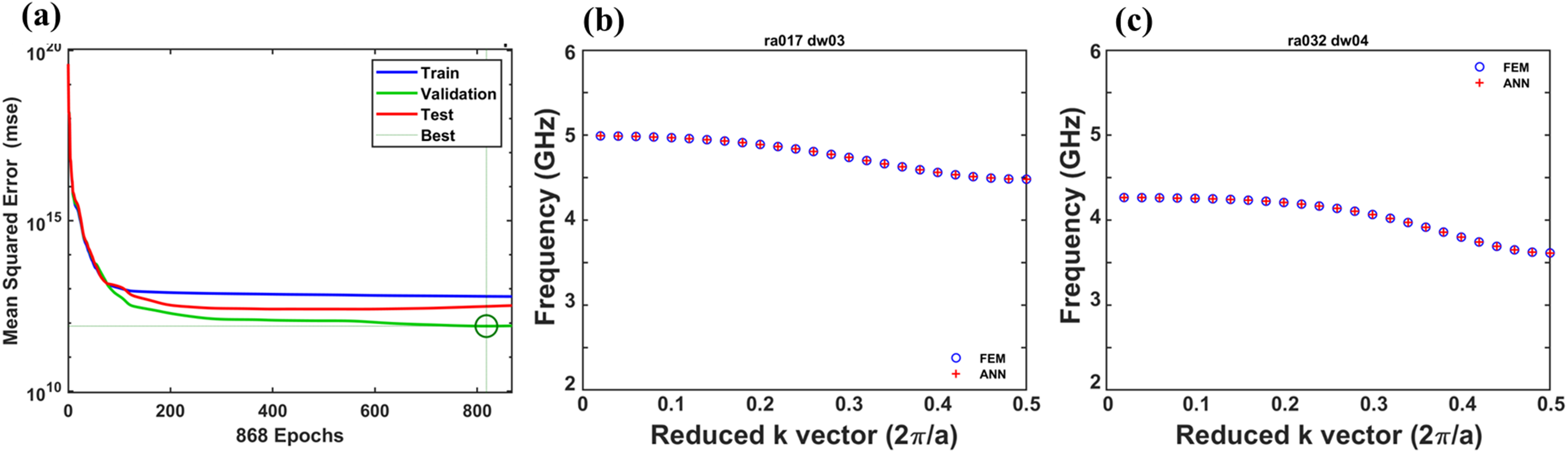
Initially, the data ratio Rd was set to 0.3, resulting in the extraction of 55 PBSs, giving $186\times 0.3\times 375=20625$ data points in total. The data points then were randomly separated into the training, validation, and testing groups with a ratio of 70:15:15 by using the software for ANN training. The training took only 185 s, and the best training, validation, and testing performances were $3.29\times {10}^{15}$ , $3.96\times {10}^{15}$ , and $4.47\times {10}^{15}$ , achieving when the number of epochs reached 564, as shown in Figure 3(a), with the performance indicated by the value of the mean square error (MSE). For illustration, Figure 3(b) and (c) show two PBSs where the points predicted using the trained ANN are compared with those calculated using the FEM. In Figure 3(b), the predicted points are represented by red + markers, and the calculated points are denoted by blue circles. The geometric parameters of this PBS, with an r/a ratio of 0.17 and a dw/w ratio of 0.3, were encompassed in the training dataset, concurrently reflecting the performance of the ANN. As depicted in the figure, the majority of the predicted points aligned well with the calculated points, barring a few discrepancies observed at the crosspoint and endpoint of the mode, circled in green.

Figure 3.

(a) ANN performance and PBS results predicted by the ANN based on Rd = 0.3 and their comparison with the results calculated using the FEM near the SS mode for (b) r/a = 0.17, dw/w = 0.3 (contained in the training dataset) and (c) r/a = 0.32, dw/w = 0.4 (not contained in the dataset).

In contrast, the PBSs presented in Figure 3(c) illustrate the prediction and calculation results for the PnC with an r/a ratio of 0.32 and a dw/w ratio of 0.4. This represents the test data that were not included in the ANN training dataset. As shown in Figure 3(c), the elastic modes exhibited frequency shifts owing to the geometric variations. Although this dataset was not part of the training set, the majority of the points aligned well, showing a performance similar to that shown in Figure 3(b). The mismatched points were also concentrated at the crosspoints and endpoints of the mode, which are marked in green. It can be seen that there are crossings in most of the green circles. Since the training dataset is composed of each of the single points, the original relationship between the points may be diluted during the training process. Therefore, in some areas where two lines should originally intersect, the ANN prediction results show two very close lines, causing the original intersection to be incorrectly predicted. This problem could be solved by increasing the complexity of the ANN configuration, meaning more hidden layers or more neurons. However, there is a trade-off between the accuracy and the training time, and there is also a risk of overfitting.

Subsequently, the data ratio Rd was increased to 0.4, resulting in the extraction of 74 datasets and 27,750 data points for training. The training took 326 s, and the best training, validation, and testing performances were $3.43\times {10}^{15}$ , $4.02\times {10}^{15}$ , and $4.12\times {10}^{15}$ , achieving when the number of epochs reached 693, as shown in Figure 4(a). Figure 4(b) and (c) illustrate the predicted and calculated PBSs, respectively, with the same geometric parameters as those in Figure 3(b) and (c). In Figure 4(b), the outcome of the data included in the training dataset, with r/a = 0.17 and dw/w = 0.3, depicted by red + markers, exhibited a better fit in the region of the green circles in Figure 3(b). However, another discrepancy emerged at an endpoint around 3.5 to 4 GHz. In contrast, the results with r/a = 0.32 and dw/w = 0.4, not included in the training dataset, are shown in Figure 4(c). Similar to Figure 4(b), although some of the mismatches in Figure 3(c) were resolved, the overall mismatch problem was more pronounced than that shown in Figure 3(c).

Figure 4.

(a) ANN performance and PBS results predicted by the ANN based on Rd = 0.4 and their comparison with the results calculated using the FEM near the SS mode for (b) r/a = 0.17, dw/w = 0.3 (contained in the training dataset) and (c) r/a = 0.32, dw/w = 0.4 (not contained in the dataset).

To obtain a more comprehensive understanding of the influence of the data ratio, the data ratio was adjusted to 0.5, and the results are shown in Figure 5. The training took 415 s, and the best training, validation, and testing performances were $3.44\times {10}^{15}$ , $3.84\times {10}^{15}$ , and $3.95\times {10}^{15}$ , achieving when the number of epochs reached 851, as shown in Figure 5(a). A comparative analysis of the outcomes achieved at Rd values of 0.3 and 0.4 revealed a notable enhancement in the performance, as displayed in Figure 5(b). This improvement is consistent with the results shown in Figure 5(c). Nevertheless, note that the crosspoints circled in green in Figure 5(c) still exhibited significant mismatches, similar to those observed in Figure 3. The persistent presence of these mismatches suggests that further investigation is required to optimize the overall predictive accuracy.

Figure 5.

(a) ANN performance and PBS results predicted by the ANN based on Rd = 0.5 and their comparison with the results calculated using the FEM near the SS mode for (b) r/a = 0.17, dw/w = 0.3 (contained in the training dataset) and (c) r/a = 0.32, dw/w = 0.4 (not contained in the dataset).

The results confirm the predictive capability of the trained ANN, albeit with room for improvement. The noted mismatches, particularly at the crosspoints, have the potential to introduce additional bandgaps or lead to inaccuracies in the mode identification, causing discontinuities in the mode points. For studies focused on extracting bandgap information from PnCs, the existing ANN requires finetuning to enhance its predictive performance. Conversely, when the objective is to explore specific resonant modes within the PBS that vary with the geometric parameters, the ANN configuration can be readily adjusted by modifying the input features, facilitating a more tailored approach to achieve accurate predictions.

To enhance the precision of the prediction of specific resonant modes within the PBS, another training dataset was achieved by pre-extracting the points of the specific mode in all of the PBSs. This results in creating a simplified “one-line” PBS (like Figure 7(b)), which serves as the input dataset for a refined ANN configuration. As illustrated in Figure 6, given that each PBS now contains a unique resonant mode corresponding to each geometric parameter set, rendering the EO feature redundant, the number of input neurons is reduced to three. The remaining layers maintain their configurations. The selected resonant mode is identified as the SS mode. Figure 1(c) and (d) show the displacement and strain fields associated with this resonant mode, respectively. This focused configuration aims to improve the accuracy of SS mode prediction by tailoring the ANN structure to the characteristics of this specific resonant feature.

Figure 6.

Configuration of the ANN designed for SS mode prediction.

Figure 7.

(a) Performance and predictions by the ANN for the SS mode based on Rd = 0.3 and their comparison with the results calculated using the FEM for (b) r/a = 0.17, dw/w = 0.3 (contained in the training dataset) and (c) r/a = 0.32, dw/w = 0.4 (not contained in the dataset).

Considering that the coordinates within the PBS represent both the reduced k vector and frequency, the slope of the mode lines can be interpreted as proportional to the group velocity of the corresponding waves. Focusing on the SS mode illustrated in Figure 1(b), denoted by the red point (with the corresponding fields in Figure 1(c) and (d)), this mode manifests as a relatively flat band in the PBS. This observation indicates that the group velocity associated with the SS mode is comparatively low within the context of the PnC.

By applying Rd = 0.3, the ANN was meticulously trained to predict the SS mode directly under various geometric parameters. The best training, validation, and testing performances were $6.04\times {10}^{12}$ , $8.08\times {10}^{11}$ , and $3.06\times {10}^{12}$ , achieving when the number of epochs reached 818, as shown in Figure 7(a). A comparison of the predicted results with the calculated results is shown in Figure 7(a) and (b). Figure 7(a) shows the performance with data points included in the training dataset (r/a = 0.17, dw/w = 0.3), whereas Figure 7(b) shows the prediction capabilities with data not included in the training dataset (r/a = 0.32, dw/w = 0.4). The figures distinctly reveal the continuous line shape characterizing the SS mode, providing an apparent representation of its evolution under different geometric conditions.

Note that the complex nature of the PBS introduces challenges, particularly concerning crossover between modes. In previous ANN training focused on the entire PBS, treating each point as an independent data point proved challenging in effectively representing crossovers. This complexity resulted in mismatches at the crossover points in Figures 3 to 5, which constitutes a primary challenge in this study. However, by training the ANN solely on data points included in specific modes, the appearance of that mode in the PBS could be distinctly observed. Figure 7(a) and (b) shows the effectiveness of this approach. The training took only 40 s, and the best validation performance of $3.46\times {10}^{12}$ was achieved when the number of epochs reached 427, showing a perfect fit between the prediction results and the actual SS mode in both the training and non-training datasets.

Discussion

According to the training results of the first network mentioned, increasing the proportion of the extracted data, as shown in Figures 3 to 5, is somewhat beneficial for the training results; however, there is no apparent relationship. Different extraction ratios may have different performances in different regions within the same PBS concentration range. This may be due to the random selection nature of the data extraction, resulting in varied training performances for different geometric ranges.

For example, at an extraction ratio of Rd = 0.4, if more data within the range of r/a = 0.15 to 0.25 are randomly selected and added to the training dataset, but fewer data are chosen in the range of r/a = 0.3 to 0.4, the performance when inputting test data with r/a = 0.32 will be poorer. When Rd was increased to 0.5, as more data were covered, having fewer training data within a specific range was less likely, which led to a higher overall fitting rate. However, in the second ANN focusing on a single mode, as only data for a single mode were included, the training information was focused on understanding the influence of the mode as the geometric parameters varied. Consequently, this ANN could predict the specified mode within the band structure varying with the structure conditions for almost any structure perfectly.

In Figure 8, the regression analysis results of the network targeting the complete PBS and the network targeting a specific mode are presented. In Figure 8(a), considering the network with Rd = 0.3 as an example, the R-value of the testing dataset (top right) is not significantly different from that of the training dataset (top left). This suggests that the network training did not encounter overfitting issues. The overall R-value (bottom right) also demonstrated a high accuracy of 0.99982, indicating that the ANN performed well for most of the data. For networks with Rd values of 0.4 and 0.5, the overall R-values were 0.99978 and 0.99982, respectively. This suggests that, in the training dataset with Rd = 0.4, the randomly extracted data may be more concentrated at specific intervals. When the data were in loosely scattered intervals, the accuracy decreased, leading to an overall decrease in accuracy. Figure 8(b) shows the regression analysis results of the ANN targeting a specific mode. The overall R-value was 1, indicating that all the training data provided correct results. This proves that the method offers excellent optimization for specific modes.

Figure 8.

Regression analysis results of the (a) ANN targeting the complete PBS with Rd = 0.3 and (b) ANN targeting the specific SS mode.

Conclusion

This study demonstrated an alternative approach for calculating the PBS of 1D PnC structures. The time needed for training the ANN is even shorter than that needed for a single calculation using the FEM (usually 5 to 10 min). Although the training time increases with the data ratio Rd, much time can still be saved once the ANN has been trained. This approach only requires the prior calculation of a small amount of the PBS, and the remaining PBS can be rapidly generated through the ANN architecture. Therefore, this method can be used in most studies conducting a PBS analysis. Moreover, based on the training results for the randomly extracted data at specific ratios, a small amount of training data should be uniformly extracted from the desired computational range. This will ensure that the information varying with the parameters is smoothly input into the ANN architecture. Additionally, if the study only needs to focus on specific resonance modes, the prediction accuracy of the ANN can be effectively increased by locking the modal data. It is anticipated that this approach will provide effective assistance for research related to PnC modal analyses.