Sage Journals: Discover world-class research

Abstract

As a new logistics technology, self-driving electric vehicles not only improve freight efficiency but also promote energy saving and emissions reductions. Aiming at logistics technologies based on self-driving electric vehicles, planning the vehicle scheduling scheme as a whole reduces energy consumption and improves economic and environmental benefits. Targeting an actual freight problem based on a two-way single-lane road connecting the pickup and delivery points and including electric charging stations, this paper proposes a method for optimizing the scheduling scenario and parameters of self-driving vehicles through computer simulations. An optimization model based on dynamic programming is established, and an optimization simulation algorithm is designed to solve the model, effectively solving the overall planning problem of vehicle scheduling. The experimental results show that the model and algorithm have good universality. After specifying an appropriate road length, total number of vehicles, number of spare vehicle batteries, duration of freight transportation, and other necessary information, the simulation algorithm is executed and the optimal scheduling scheme and the total amount of freight transported are output. The efficiency of the algorithm is extremely high, requiring only 1.5 s to complete the whole simulation process of scheduling 150 vehicles for 1000 h over a road with a length of 10 km.

Keywords

logistics engineering vehicle dispatching self-driving electric vehicle dynamic programming simulation algorithm overall planning

Introduction

Self-driving electric vehicles have been widely studied for their potential to greatly improve freight efficiency and promote carbon emission reduction and resource conservation. Several scholars have researched scheduling methods for unmanned transport vehicles. Hong et al.¹ studied a scheduling method for unmanned electric trucks on roads within port areas, while Zhang et al.² explored the scheduling mechanism of unmanned vehicles at intersections. However, there has been little research on the transportation scheduling and charging issues of unmanned electric transport vehicles on highways. This article presents a typical case study of a bidirectional single-lane highway system and proposes an efficient scheduling method for driverless electric transport vehicles as a general solution to such problems. The proposed method is based on a dynamic programming model. A simulation algorithm is designed to solve the model, and a scheduling scheme that improves transportation efficiency and reduces resource redundancy is developed. Finally, the reliability of the scheme is verified by a series of visualization methods.

Literature review and our work

Vehicle scheduling³ is a complex combinatorial optimization problem,⁴ which makes it difficult to analyze from the perspective of general mathematical theory and often requires computational approaches. Wang et al.⁵ used a multiobjective genetic algorithm to study dynamic bus scheduling in traffic congestion as an effective means of dealing with traffic congestion. Shui et al.⁶ explored the application of a clonal selection algorithm in bus scheduling, allowing satisfactory scheduling schemes to be generated in a short time. Sowmya et al.⁷ studied an optimal management strategy for vehicle scheduling and charging and used intelligent optimization algorithms in the process. However, these studies mainly focus on urban transportation, and unmanned vehicles are currently difficult to apply in such environments. Due to the complexity of the road network and the uncertainties associated with the road surface, it is extremely difficult for unmanned vehicles to carry out global scheduling and planning. However, in a simple two-way single-lane road structure with relatively few interference factors, the application of unmanned vehicles is more effective and can achieve greater efficiency.

Computer simulations⁸ recreate real-world situations through mathematical models. They have been widely used in various industries, such as architectural design,⁹ social practice,¹⁰ material science,¹¹ engineering mechanics,¹² and life sciences,¹³ to study the core nature of a problem at the data level and are typically easy to check and verify. Malysza et al.¹⁴ used computer simulation technology to optimize the casting process, while Durgut et al.¹⁵ employed simulation and optimization techniques in a hydrological model to improve the prediction performance. Kenett et al.¹⁶ have discussed the importance of computer simulations in the new industrial era. These works all demonstrate that computer simulation plays an important role in people's daily life and production. However, there is currently relatively little research on computer simulation methods for self-driving vehicle scheduling systems. The present paper considers a mathematical programming problem. By applying a simulation algorithm, a mobile scheduling scheme is developed for unmanned electric material transport vehicles on a two-way single-lane road. The scheme is applied to the control of vehicles between the pickup point, the delivery point, and two power stations. An optimization method is applied to the scheduling scheme to maximize the amount of cargo transported and minimize the number of battery changes.

Symbol definition

Table 1 summarizes all the mathematical symbols that appear in the paper.

Table 1.

Symbols and explanations.

Symbol	Meaning
i	Number of power station
j	Number of vehicle spaces in the conveyor belt model
LR	The total length of the road connecting the pickup and unloading points
VC	Rated speed of the self-driving vehicles
LC	Minimum distance between self-driving vehicles
NC	Initial total number of vehicles
NB	Initial total number of batteries
DEU	Power consumption speed when the vehicle is not loaded
DEL	Power consumption speed of the vehicle when carrying goods
DET	The total power consumption of driving on the conveyor belt for one cycle
MinS	Minimum remaining electricity allowed to return to the power station
MaxS	Maximum remaining electricity allowed to return to the power station
TB	The time it takes to fully charge a set of car batteries
TL	Time required for loading goods
TU	Time required for unloading goods
TotalT	Total transportation time
NG	The maximum total number of vehicles on the pickup route
NP	The maximum total number of vehicles that can enter the pickup station
NB	The maximum total number of vehicles on the delivery route
ND	The maximum total number of vehicles that can enter the delivery station
P_i	The vehicle space number corresponding to power station i
M_i	The number of battery packs initially assigned to power station i
MinT_i	The minimum number of times that an electric vehicle starting from the i-th power station can return to the station to charge
MaxT_i	The maximum number of times that an electric vehicle starting from the i-th power station can return to the station to charge
CS_i	The electric vehicle power consumption from the i-th power station to the other power station
IC_jt	Whether there is a vehicle in the j-th vehicle space when the t-th vehicle space move occurs.
BKit	A 0-1 variable represents whether there is a vehicle that needs to be returned to the power station for charging when the i-th power station moves in the t-th vehicle space
RcEit	The total number of vehicles that can be dispatched from the i-th station on the t-th vehicle space move
BC_jt	The number of times that the vehicle in the j-th vehicle space needs to pass through the station on the t-th vehicle space move
UcE_it	The total number of vehicles for which the battery has not been swapped at the i-th power station at the time of the t-th vehicle space move
RbE_it	The total number of batteries filled by the i-th power station at the t-th vehicle space move
G	Number of battery packs equipped on a car
RC	The number of times the vehicle space moves in the time required to replace the battery

Problem description

Consider a two-way single-lane road, with the pickup point C at one end and the delivery point D at the other end. A batch of automatic electric vehicles transports materials cyclically from point C to point D, returning to point C with no load. There are power stations P₁ and P₂ at the midpoint of points C and D, one on either side of the road. The electric vehicles enter the power station for battery replacement when they have low power. Batteries with unsatisfactory power can be charged in the power station via either fast charging or slow charging, which are realized by two different charging piles. We require a scheduling scheme for vehicles and battery packs that maximizes the amount of materials transported within a specified time period. Under this premise, the number of planned fast-charging piles should be as small as possible to meet resource constraints and battery operation mode constraints.

For this basic problem, we test the reliability and universality of the model under the following assumptions:

Route: The mileage from the start point C to the end point D of this section of highway is a constant LR. The power stations P₁ and P₂ are located between points C and D and are set on opposite sides of the road. Vehicles can only enter the power station on the same side of the road to replace their batteries.

Driving: The driving speed of the unmanned electric vehicles is fixed at VC km/h. Acceleration and deceleration are ignored. The distance between successive vehicles should not be less than a constant LC.

Schedulable resources: There are NC initial vehicles, each equipped with a set of G onboard batteries. Vehicles have a total of NB spare onboard batteries.

Transport volume: Suppose that the smallest unit of cargo is “one car of goods.” The completion of loading at point C and unloading at point D by the electric vehicle is recorded as the transportation of one car of goods.

Power consumption and charging: The power consumption of the vehicles depends on whether they are running “unloaded” or “loaded.” The unloaded power consumption rate is DEU %SOC/min, while the loaded power consumption rate is DEL %SOC/min. To avoid repeated charging and flameout, the power must be between MinS and MaxS before the vehicle can return to a power station. The slow charging pile requires time TB to fill a set of batteries, while the fast charging pile requires less than TB. The number of slow-filling piles is sufficient, and the number of fast-charging piles is determined as part of the solution.

Time consumption: The loading and unloading of processes and the replacement of batteries are all automated. The loading time is TL and the unloading time is TU. The battery replacement time is TC.

Total running time: The total running time is TotalT.

According to the above assumptions, a model is established and an optimization algorithm is implemented. The total amount of goods transported, the number of battery changes, and the optimal scheduling scheme are output.

Establishment of traffic flow conveyor belt model

The conveyor belt model is appropriate for vehicles driving along with a two-way single-lane highway.^17,18 First, we determine the location of the power stations, and then we optimize the scheduling of the electric transport vehicles and carry out loading and unloading at points C and D, respectively.

The vehicles traveling in the same direction on the two-way road need to maintain a minimum distance. We set this distance to LC and neglect the length of each vehicle (see Figure 1).

Figure 1.

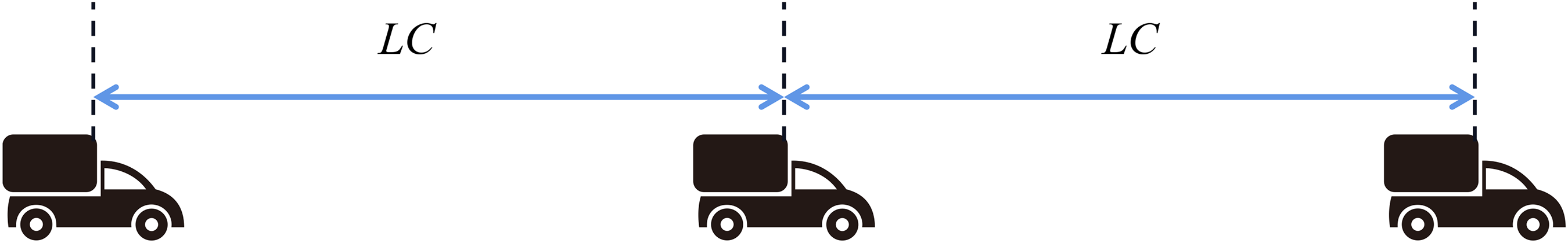
Diagram of maximum vehicle density.

In maximizing the transport efficiency, it is theoretically possible to schedule all vehicles with a minimum spacing of LC (as in Figure 1). Empty vehicles are dispatched from the initial power station at intervals of LC. Each vehicle heads to the loading station, loads materials, and then heads to the unloading station. After the materials have been unloaded, the vehicle returns to the loading station on the other side of the road at a fixed speed (as shown in Figure 2). In this way, the transportation line can transport goods with maximum efficiency.

Figure 2.

Schematic diagram of maximum density dispatching (maximum efficiency transportation).

If we regard the two processes of loading at the pickup point and unloading at the delivery point as moving at a constant speed, we can calculate the total number of vehicles that can be dispatched at the shortest distance in a loading and unloading time by converting the time of loading and unloading to the distance the vehicle would move at its constant speed.

Recall that TL is the time required to load the goods, TU is the time required to unload the goods, LC is the minimum distance between vehicles, and VC is the rated speed of the electric vehicles. Thus:

Number of departures while loading = ⌈ T L / \frac{L C}{V C} ⌉

(1)

Number of departures while unloading = ⌈ T U / \frac{L C}{V C} ⌉,

(2)where the operator

⌈ ⌉

represents rounding up.

Let LR be the total length of the highway. Then, the maximum number of vehicles moving in one direction is calculated as follows:

Maximum number of driving on road = ⌊ \frac{L R}{L C} ⌋,

(3)where the operator

⌊ ⌋

represents rounding down.

As shown in Figure 3, the electric vehicles move clockwise around the entire road network, as on a conveyor belt. Therefore, we name this the “conveyor belt model.” Each vehicle on the conveyor belt is called a “vehicle space.” The whole transportation process is regarded as several vehicle spaces being transmitted clockwise on a conveyor belt of length LR.

Figure 3.

Numbering method of vehicle spaces on the conveyor belt.

To describe the conveyor belt model in more detail, each vehicle space on the conveyor belt is numbered. As shown in Figure 3, we start with the vehicle moving from the unloading station D to the pickup station C. The initial vehicle space is numbered 1. Next, we set NG as the maximum total number of vehicles on the pickup route, set NP as the maximum total number of vehicles that can enter the pickup platform during the time required at the pickup station to load goods, set NB as the maximum total number of vehicles on the delivery route, and set ND as the maximum total number of vehicles that can enter the delivery platform during the time required to unload the goods. Therefore, the total number of vehicle spaces is NG + NP + NB + ND; these are numbered according to the driving direction of the electric vehicles. These four variables are calculated as follows:

N G = N B = ⌊ \frac{L R}{L C} ⌋

(4)

N P = ⌈ T L / \frac{L C}{V C} ⌉

(5)

N D = ⌈ T U / \frac{L C}{V C} ⌉

(6)To facilitate the description of the actual running state of each vehicle space (with or without cars), we set an iterative variable j to represent the number of each vehicle space. The range of j is as follows:

1 \leq j \leq N G + N P + N B + N D, j \in Z

(7)Let P_i be the vehicle space number corresponding to power station i, where i = 1 for the power station on the pickup road and i = 2 for the power station on the delivery road. That is, P₁ and P₂ represent the vehicle space numbers of power stations 1 and 2, respectively. Power station 1 is located in the pickup direction, when the vehicle is carrying no load, and power station 2 is located in the delivery direction, when the vehicle is fully loaded. Thus, P₁ and P₂ meet the following constraints:

1 \leq P_{1} \leq N G

(8)

N G + N P + 1 \leq P_{2} \leq N G + N P + N B

(9)

P_i is one of the decision variables, and the above constraint will be given again in the model for the problem.

The actual distance of each vehicle on the road can be understood as the forward movement of all vehicle spaces on the conveyor belt, which is recorded as a “vehicle space move.” A vehicle space moving along with the forward direction takes a time of LC/VC. The vehicle space number does not move with the vehicle space and is fixed on the conveyor belt. After each vehicle space movement, all vehicles on the conveyor belt pass to the vehicle space immediately in front. The vehicle in the last numbered vehicle space moves to the starting point.

In addition to the need to determine the location of the power station, it is also important to clarify the distribution of the reserve battery packs in the two power stations in the initial state. Let M_i be the number of battery packs initially assigned to power station i. Then, the sum of the initial battery packs at the power stations satisfies:

\sum_{i = 1}^{2} M_{i} = N B, M_{i} \in N

(10)where NB is the total amount of batteries and NC represents the total number of vehicles.

We now consider scheduling analysis on the basis of the conveyor belt model. Vehicle scheduling aims to determine when to dispatch an electric vehicle from the power station, when the vehicle should return to the power station, and when the battery of the electric vehicle should be replaced. Based on this problem, the vehicle scheduling can be summarized in terms of the three decision variables listed in Table 2.

Table 2.

Main decision variables.

Symbol	Meaning
OE_it	Whether the i-th power station sends an electric vehicle when the t-th vehicle space moves. This is a 0–1 variable, with 1 representing a dispatch and 0 representing no dispatch.
BE_it	The number of times that the electric vehicle sent by the i-th power station can pass the power station before returning for charging during the t-th vehicle space movement. If the car is not dispatched when vehicle space t moves, the variable value defaults to 0.
CcE_it	Whether the i-th power station replaces the battery of the electric vehicle during the t-th vehicle space movement. This is a 0–1 variable, with 1 representing yes and 0 representing no. If there is no electric vehicle to be replaced in the station when vehicle space t moves, the variable value defaults to 0.

Note: Iteration variable i = 1, 2 represents power stations 1 and 2. The iteration variable t = 1, 2, … represents the number of vehicle space moves, which continue until the last vehicle space move at the end of the simulation time.

Each vehicle space is either “occupied” or “unoccupied.” In the initial state, all vehicle spaces are unoccupied and begin to move clockwise. As an unoccupied vehicle space passes a power station, the station can decide whether to dispatch an electric vehicle.

There are many states in the driving process of the electric vehicles: no-load driving (low power consumption), loading and unloading (no power consumption, parking, and waiting), loaded driving (high power consumption), battery replacement (no power consumption, parking, and waiting). In our conveyor belt model, we regard loading and unloading as a vehicle running on the conveyor without power consumption. Therefore, the process on the conveyor belt includes no-load driving, loaded driving, loading, and unloading but does not include replacing the battery.

Because the vehicle can only have its battery replaced when it passes through the power station, we simplify the model by only considering the battery state of the vehicle as it passes through the power station; that is, we do not consider the battery state while the vehicle is driving. Therefore, we only predict that the vehicle can pass the power stations several times when it is dispatched and replace the battery after the vehicle has passed the power stations several times.

Let DEL be the power consumption of driving for 1 min when loaded and let DEU be the power consumption of driving for 1 min in the no-load condition. The total power consumption of driving on the conveyor belt for one cycle is DET. The general formula for calculating the power consumption of one cycle is as follows:

D E T = \frac{L R}{V C} \cdot (D E L + D E U)

(11)A schematic diagram of power consumption over one cycle is shown in Figure 4.

Figure 4.

Schematic diagram of power consumption.

For battery swapping, our hypothesis stipulates that the power of the electric vehicle must be below a certain level before it returns to the power station. We set the variable MaxS as the upper limit of the power allowed by the electric vehicle and MinS as the lower limit of the power allowed by the electric vehicle, that is, the SOC of the onboard battery must be in the range [MinS, MaxS] before entering the power station for battery swapping. The power stations are located on the roadside in both directions, that is, the vehicle will pass through the power station twice in a cycle (Figure 5). As long as the power is in [MinS, MaxS], vehicles can enter either power station. As mentioned above, we only care about the remaining electricity when the vehicle passes through the power station. After an electric vehicle leaves either power station, according to the position set by the power station, the vehicle is assumed to pass through that power station for the first time. The amount of electricity consumed before the battery should be replaced and the number of times a vehicle passes a power station before satisfying the battery swapping requirements can then be calculated. Any integer can be used as the maximum number of times that the electric vehicle passes through a power station after departure.

Figure 5.

Vehicles passing through the power stations and CS₁, CS₂ in a cycle.

The variable MinT_i is the minimum number of times that an electric vehicle starting from the i-th power station can return to the station to charge, and MaxT_i is the maximum number of times that an electric vehicle starting from the i-th power station can return to the station to charge. When making the decision whether to send a vehicle out onto the highway, we must also determine when the electric vehicle will return to the station for charging after several cycles. Therefore, we set the decision variable BE_it as:

M a x T_{i} \leq B E_{i t} \leq M i n T_{i}, B E_{i t} \in Z .

(12)We set the variable CS_i to represent the electric vehicle power consumption from the i-th power station to the other power station. Then, the calculation formula for CS_i is as follows:

C S_{1} = \frac{L R - (P_{1} - 1) L C}{V C} \cdot D E U + \frac{(P_{2} - N G - N P - 1) L C}{V C} \cdot D E L

(13)

C S_{2} = \frac{(P_{1} - 1) L C}{V C} \cdot D E U + \frac{L R - (P_{2} - N G - N P - 1) L C}{V C} \cdot D E L,

(14)where CS₁ and CS₂ are illustrated in Figure 5.

Then, MinT_i and MaxT_i satisfy the following equations:

M a x T_{i} = m a x {x | x \leq 1 - M i n S a n d (x = β C S_{1} + β C S_{2} o r x = β C S_{1} + β C S_{2} + C S_{i}), β \in Z}

(15)

M i n T_{i} = m i n {x | x \geq 1 - M a x S a n d (x = β C S_{1} + β C S_{2} o r x = β C S_{1} + β C S_{2} + C S_{i}), β \in Z}

(16)In summary, the general framework of the conveyor belt model is as follows:

s . t . {\begin{matrix} N G = N B = ⌊ \frac{L R}{L C} ⌋ \\ N P = ⌈ T L / \frac{L C}{V C} ⌉ \\ N D = ⌈ T U / \frac{L C}{V C} ⌉ \\ 1 \leq j \leq N G + N P + N B + N D, j \in Z \\ 1 \leq P_{1} \leq N G, P_{1} \in Z \\ N G + N P + 1 \leq P_{2} \leq N G + N P + N B, P_{2} \in Z \\ C S_{1} = \frac{L R - (P_{1} - 1) L C}{V C} \cdot D E U + \frac{(P_{2} - N G - N P - 1) L C}{V C} \cdot D E L \\ C S_{2} = \frac{(P_{1} - 1) L C}{V C} \cdot D E U + \frac{L R - (P_{2} - N G - N P - 1) L C}{V C} \cdot D E L \\ M a x T_{i} = max {x | x \leq 1 - M i n S a n d (x = β C S_{1} + β C S_{2} \\ o r x = β C S_{1} + β C S_{2} + C S_{i}), β \in Z} \\ M i n T_{i} = min {x | x \geq 1 - M a x S a n d (x = β C S_{1} + β C S_{2} \\ o r x = β C S_{1} + β C S_{2} + C S_{i}), β \in Z} \\ \sum_{i = 1}^{2} M_{i} = N B, M_{i} \in N \end{matrix}

With the exception of equation (13), the variable BE_it is used as a dynamic programming model variable, as will be explained in the following modeling process.

Establishment of vehicle scheduling dynamic programming model

We consider the electric vehicle scheduling problem over a period of 1000 h. Due to the excessive number of vehicle space moves in a long period of time, it is difficult to perform a global one-time optimization. Therefore, we establish a dynamic programming model to pursue each vehicle space move. The global situation of the vehicle scheduling is estimated and evaluated. The multiobjective dynamic programming model of hierarchical optimization is established with the maximum traffic volume as the first optimization goal and the minimum charging time as the second optimization goal.

Objective Function 1: Maximize transport volume:

min f_{1} = \sum_{t = 1}^{T m a x} I C_{e n d P, t}

(17)where IC_jt represents whether there is a vehicle in the j-th vehicle space when the t-th vehicle space move occurs. This is a 0–1 variable, with 1 representing yes and 0 representing no. The final vehicle space is numbered endP and is located at the last point of unloading at the unloading station. The meaning of Tmax is the total number of vehicle space moves that occur within a stipulated time. The total number of vehicles passing through this position during the stipulated time can be counted to calculate the amount of goods transported. The calculation formulas for Tmax and endP are as follows:

T m a x = T o t a l T / \frac{L C}{V C}

(18)

e n d P = N G + N P + N B + N D

(19)

where TotalT is the total time stipulated for operation.

Objective Function 2: Minimize number of charging times for the battery pack:

min f_{2} = \sum_{i = 1}^{2} \sum_{t = 1}^{T m a x} B K_{i t}

(20)where BK_it represents whether there is a vehicle that needs to be charged when the i-th power station moves in the t-th vehicle space. A value of 1 represents yes and a value of 0 represents no. As the electricity bill will not change over time, we assume that once the vehicle returns to the station and there is a residual battery, the vehicle battery will be replaced and the battery will be charged immediately.

After each charging of the battery pack, maintenance is required, which will increase the labor cost. The number of charging times should be minimized while maintaining the maximum traffic volume. From the perspective of dynamic programming, each vehicle should travel for as long as possible. ➢

Dispatch electric vehicle constraints

This part of the constraint is directly related to the scheduling of electric vehicles. The decision variables OE_it and BE_it determine whether the vehicle is dispatched each time a vehicle space passes through the power station and the period until the vehicle must return to the power station.

Constraint 1: Whether the power station dispatches the vehicle.

OE_it: When the t-th vehicle space move occurs, this variable determines whether the vehicle is dispatched from the i-th station, with 1 representing yes and 0 representing no.

RcE_it: This variable indicates the total number of vehicles that can be dispatched from the i-th station to the t-th vehicle space move.

When there is a car in the vehicle space of the power station, or when there is no outbound vehicle at the power station, no car can be dispatched:

O E_{i t} = 0, i f I C_{P_{i}, t} = 1 o r R c E_{i t} = 0. O E_{i t} \in {0, 1}

(21)Moreover, in the initial state, all vehicles must be dispatched from power station 1:

R c E_{1, 0} = N C

(22)where NC represents the total number of vehicles.

When a vehicle space passes through the power station, the decision as to whether to dispatch a vehicle must first consider whether the vehicle space is unoccupied, and then whether there is at least one vehicle equipped with a full battery in the power station that is ready to be dispatched. If both conditions are satisfied, a vehicle can be dispatched; otherwise, no vehicle is dispatched.

Constraint 2: Decide the length of vehicle travel.

BE_it indicates that the i-th power station replaces the battery when the vehicle passes the t-th vehicle space move and dispatches the vehicle. This variable is an integer decision variable that determines the driving time of the dispatched vehicle. The value of this variable can only be determined when the vehicle is dispatched.

The vehicles return to a power station to replace their batteries according to certain power requirements. The constraint formula is given by equation (12) in the conveyor belt model and is repeated here for completeness:

M a x T_{i} \leq B E_{i t} \leq M i n T_{i}, B E_{i t} \in Z

(23)Constraint 3: Record and update the number of times a vehicle must return to a power station.

BC_jt: The number of times that the vehicle in the j-th vehicle space needs to pass through the station on the t-th vehicle space move. The value is initially generated at the time of departure. During the driving process, the variable decreases by one each time the battery is charged. The battery is replaced when the value reaches 0.

The number of times the vehicle needs to pass through the power station is limited to the value determined at the time of dispatch:

B C_{P_{i}, t} = B E_{i t}, i f O E_{i t} = 1

(24)When the value reaches 0, the vehicle returns to the station:

B K_{i t} = {\begin{matrix} 1, i f B C_{P_{i}, t} = 0 \\ 0, e l s e \end{matrix}

(25)Constraint 4: Update vehicle space information.

Once a vehicle is dispatched, the vehicle space at which the power station is located is limited to the occupied state:

I C_{P_{i}, t} = 1, i f O E_{i t} = 1

(26)

➢

Electric vehicle driving constraints

Constraint 5: After the vehicle space moves, the information on all vehicles at the station is updated. The number of times the updated vehicle needs to pass through the power station is:

B C_{P_{i}, t} = B C_{P_{i} - 1, t - 1} - 1, i f O E_{i t} = 0 a n d I C_{P_{i} - 1, t - 1} = 1.

(27)The vehicle existence information of the vehicle space at which the power station is located is updated as:

I C_{P_{i}, t} = I C_{P_{i} - 1, t - 1} - 1, i f O E_{i t} = 0 a n d I C_{P_{i} - 1, t - 1} = 1.

(28)The above two equations are only valid for vehicles passing through the station, and OE_it must be equal to 0, that is, the station does not dispatch new vehicles at this time. If vehicle replacement occurs, the information on the vehicle space is covered by the newly dispatched electric vehicle information.

If P_i = 1, then:

B C_{1, t} = B C_{e n d P, t - 1} - 1, i f O E_{1, t} = 0 a n d I C_{e n d P, t - 1} = 1

(29)

I C_{1, t} = I C_{e n d P, t - 1} - 1, i f O E_{1, t} = 0 a n d I C_{e n d P, t - 1} = 1.

(30)This is because the previous vehicle space numbered 1 is the last space. Vehicles not passing through the station are subject to the following constraints.

Constraint 6: After the vehicle space moves, the new location information of the vehicle is updated:

B C_{j t} = B C_{j - 1, t - 1}, j \neq P_{i}

(31)

I C_{j t} = I C_{j - 1, t - 1}, j \neq P_{i} .

(32)This constraint is only valid for vehicles that are not passing through a station. Additionally, the last vehicle space will be moved to vehicle space 1:

B C_{1, t} = B C_{e n d P, t - 1}, j \neq P_{i}

(33)

I C_{1, t} = I C_{e n d P, t - 1}, j \neq P_{i} .

(34)

➢

Battery swapping constraints for electric vehicles

Constraint 7: Vehicles are subjected to battery swapping constraints.

UcE_it: The total number of vehicles for which the battery has not been swapped at the i-th power station at the time of the t-th vehicle space move.

CcE_it: The total number of vehicles that started battery replacement at the i-th power station at the time of the t-th vehicle space move. This is a decision variable, with each vehicle space move determining whether the vehicle battery requires replacement. However, it is theoretically more advantageous to replace the battery as soon as possible:

U c E_{i t} = U c E_{i, t - 1} - C c E_{i t} + B K_{i t} .

(35)Constraint 8: Limit the number of cars that can have their battery replaced.

RbE_it: The total number of batteries filled by the i-th power station at the t-th vehicle space move.

G: Number of battery packs equipped on a car.

At least six sets of full batteries are required for each vehicle battery replacement:

C c E_{i t} \leq \frac{R b E_{i t}}{G}, C c E_{i t} \in N .

(36)Constraint 9: Update the number of cars after battery replacement.

TC: Time required to replace the vehicle battery.

RC: The number of times the vehicle space moves in the time required to replace the battery.

The formula for RC is as follows:

R C = T C / \frac{L C}{V C},

(37)where LC is the distance between the two vehicle spaces and VC is the vehicle speed. These values are given in the conveyor belt model.

If the battery is swapped at the time of the t-th vehicle space move, the vehicle can exit again at the time of the (t + RC)-th vehicle space move. The total number of outbound vehicles from the i-th power station after the battery swapping is updated as follows:

R c E_{i t} = R c E_{i, t - 1} + C c E_{i, t - R C}, t > R C .

(38)

➢

Battery charging constraints

Constraint 10: Initialize the number of batteries in the power station:

R b E_{i, 0} = M_{i} .

(39)Constraint 11: Update power station battery information when replacing onboard batteries.

TB: Total time required for battery charging, maintenance, etc.

RB: The number of times the vehicle space moves during the time required for a battery charge:

R B = T B / \frac{L C}{V C} .

(40)The total number of outbound vehicles from the i-th power station after battery swapping is calculated as follows:

R b E_{i t} = {\begin{matrix} R b E_{i, t - 1} - G \cdot C c E_{i, t}, t \leq R B \\ R b E_{i, t - 1} - G \cdot C c E_{i, t} + G \cdot C c E_{i, t - R B}, t > R B \end{matrix},

(41)where CcE_it is the total number of vehicles currently undergoing battery replacement and CcE_i,_t−RB is the number of batteries unloaded and charged before the RB-th move. Each battery is charged immediately after being unloaded from the electric vehicle and is added to the total amount of available batteries after the RB-th vehicle space move.

In summary, the overall mathematical model of the inner dynamic programming is as follows:

m i n f_{1} = \sum_{t = 1}^{T m a x} I C_{e n d P, t}

m i n f_{2} = \sum_{i = 1}^{2} \sum_{t = 1}^{T m a x} B K_{i t}

s . t . {\begin{matrix} O E_{i t} = 0, i f I C_{P_{i}, t} = 1 o r R c E_{i t} = 0, O E_{i t} \in {0, 1} \\ R c E_{1, 0} = N C, R b E_{i, 0} = M_{i} \\ M a x T_{i} \leq B E_{i t} \leq M i n T_{i}, B E_{i t} \in Z \\ B C_{P_{i}, t} = B E_{i t}, i f O E_{i t} = 1 \\ I C_{P_{i}, t} = 1, i f O E_{i t} = 1 \\ B C_{P_{i}, t} = B C_{P_{i} - 1, t - 1} - 1, i f O E_{i t} = 0 a n d I C_{P_{i} - 1, t - 1} = 1 \\ I C_{P_{i}, t} = I C_{P_{i} - 1, t - 1} - 1, i f O E_{i t} = 0 a n d I C_{P_{i} - 1, t - 1} = 1 \\ B C_{1, t} = B C_{e n d P, t - 1} - 1, i f O E_{1, t} = 0 a n d I C_{e n d P, t - 1} = 1 \\ I C_{1, t} = I C_{e n d P, t - 1} - 1, i f O E_{1, t} = 0 a n d I C_{e n d P, t - 1} = 1 \\ B C_{j t} = B C_{j - 1, t - 1}, j \neq P_{i} \\ I C_{j t} = I C_{j - 1, t - 1}, j \neq P_{i} \\ B C_{1, t} = B C_{e n d P, t - 1}, j \neq P_{i} \\ B K_{i t} = {\begin{matrix} 1, i f B C_{P_{i}, t} = 0 \\ 0, e l s e \end{matrix} \\ I C_{1, t} = I C_{e n d P, t - 1}, j \neq P_{i} \\ U c E_{i t} = U c E_{i, t - 1} - C c E_{i t} + B K_{i t} \\ C c E_{i t} \leq \frac{R b E_{i t}}{G}, C c E_{i t} \in N \\ R C = ⌈ T C / \frac{L C}{V C} ⌉ \\ R c E_{i t} = R c E_{i, t - 1} + C c E_{i, t - R C}, t > R C \\ R B = ⌈ T B / \frac{L C}{V C} ⌉ \\ R b E_{i t} = {\begin{matrix} R b E_{i, t - 1} - G \cdot C c E_{i, t}, t \leq R B \\ R b E_{i, t - 1} - G \cdot C c E_{i, t} + G \cdot C c E_{i, t - R B}, t > R B \end{matrix} \\ e n d P = N G + N P + N B + N D \\ T m a x = T o t a l T / \frac{L C}{V C} \end{matrix}

Based on the above model, an algorithm is developed to solve the optimal transportation scheduling problem.

Solution algorithm

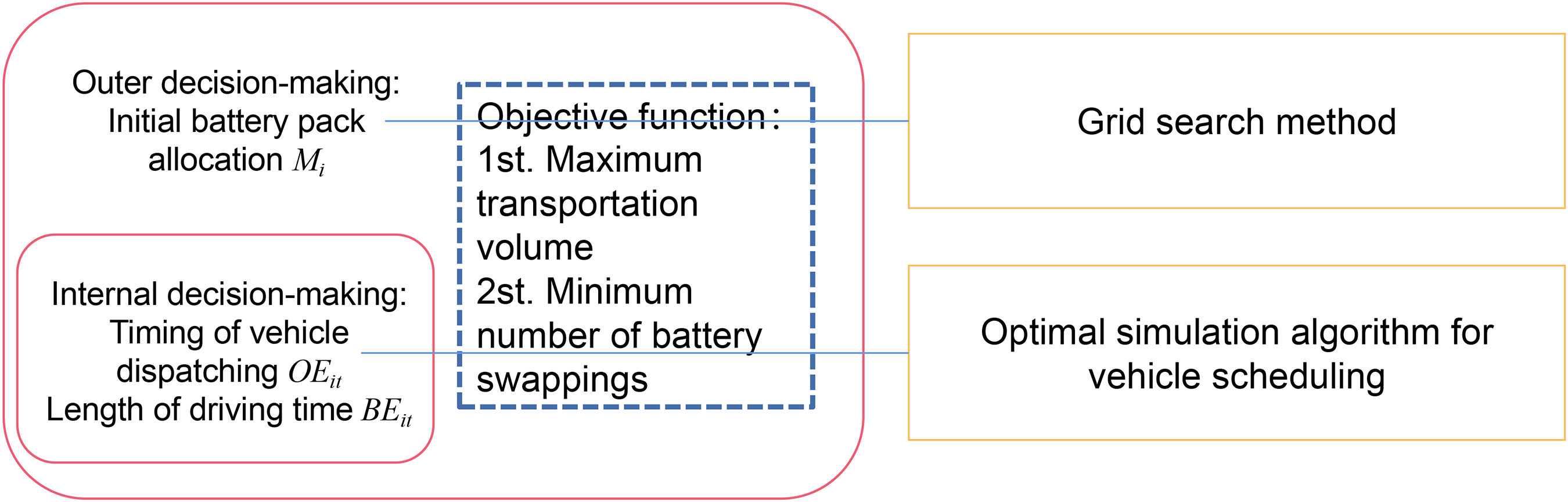
To solve the model, we design the following algorithm. The core algorithm involves vehicle scheduling. The algorithm needs to input all known parameters and determine the initial number of battery packs, from which we obtain the optimal scheduling scheme for determining M_i extremely quickly (computation time of about 1 s).

This algorithm returns the optimal decision variables OE_it and BE_it, whereupon a grid method can be applied to determine the optimal M_i in the outer layer of the algorithm. An outline of the algorithm is shown in Figure 6.

Figure 6.

Solution algorithm structure.

The full search of the M_i distribution is simple. The pseudo-code for the grid search method and its implementation is provided in the Supplementary Materials. The following briefly introduces the optimal simulation algorithm for vehicle scheduling: ➢

Optimal simulation algorithm for vehicle scheduling

The algorithm achieves the best scheduling arrangement. The core idea mainly lies in the following two points:

The stable optimal cycle is estimated based on the known data, that is, a vehicle scheduling scheme cycle that can run in a relatively limited time with the maximum traffic volume and the minimum number of power changes. Repeating this scheme over an infinite time will achieve the best scheduling effect.

Plan the best initial departure strategy. The global vehicle layout defines the optimal cycle in the shortest time.

The algorithm flowchart is shown in Figure 7.

Figure 7.

Flowchart of the optimal simulation algorithm.

See Supplementary Materials “Annex I” and “Annex II” for the specific pseudo-code.

Simulation calculations and results analysis

The model is a multiobjective programming model. We solve the two optimization objectives using a linear weighting method. We then standardize, weigh, and sum the two objective function values and take the minimum comprehensive objective function as the final optimization objective. For the two objective functions, we believe that the importance of maximizing the traffic volume is much greater than the number of battery charging times, so the weight of the first objective function is set to 0.99, and the weight of the second objective function is set to 0.01.

To study the feasibility and generalization ability of the model, we consider several sets of parameters and analyze the results. The parameter combinations are listed in Table 3.

Table 3.

Three groups of parameter combinations.

Meaning	Symbol	Group 1	Group 2	Group 3
Highway length (km)	LR	10	15	20
Fixed vehicle spacing (m)	LC	200	180	220
Number of electric vehicles	NC	125	150	175
Rated speed of electric vehicles (km/h)	VC	60	70	70
Number of battery packs equipped with an electric vehicle	G	6	6	6
Number of backup battery packs	NB	150	90	210
Power consumption speed at no load (%SOC/min)	DEU	1/3	1/3	1/3
Power consumption speed at full load (%SOC/min)	DEL	1/2	1/2	1/2
Time for slow charging pile to fully charge the battery (h)	TB	3	3	3
Total duration of operation (h)	TotalT	1000	1000	1000
Time required for loading (min)	TL	1	3	4
Time required for unloading (min)	TU	1	3	4
Time required to replace the car battery (min)	TC	1/3	1	1
Minimum remaining power when returning to the station	MinS	10%	10%	5%
Maximum remaining power when returning to the station	MaxS	25%	25%	20%

The default locations for the two power stations are at the midpoints of the roads running in each direction between points P and D. The solution algorithm is executed using the three sets of parameters in Table 2, and three different sets of results and runtimes are obtained. The results are presented in Table 4.

Table 4.

Best solution result without quick-filling piles.

	Group 1	Group 2	Group 3
Maximum plan freight volume	228833	153682	148627
Optimal number of battery swaps	21750	19108	22854
Initial battery pack allocation (Station 1/Station 2)	72/78	60/0	102/108
Program runtime (s)	1.5778	1.5942	1.7622

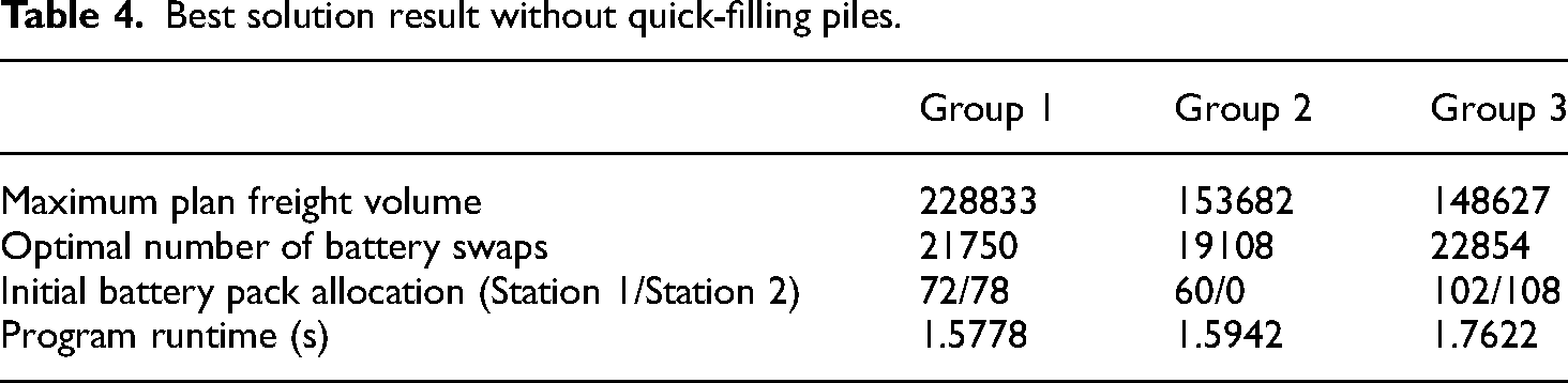
The results show that the algorithm can quickly calculate solutions under different model parameter combinations and that the model has good generalization ability.

A real coded genetic algorithm¹⁹ was also used to solve this optimization problem. Taking the Group 1 parameter combination as an example, 300,000 vehicle space moves require a total of 1000 h of simulation time. The decision variable is whether to dispatch vehicles as the 300,000 vehicle spaces pass through the power station, which is regarded as the phenotype of the solution. The optimized solution is determined through the genetic algorithm. A comparison of the solutions is presented in Table 5.

Table 5.

Comparison of solution effects between optimal simulation algorithm and genetic algorithm.

	Optimal Simulation Algorithm	Genetic Algorithm
Maximum plan freight volume	228833	198946
Optimal number of battery swaps	21750	19202
Initial battery pack allocation (Station 1/Station 2)	72/78	72/78
Program runtime (s)	1.5778	10.7796

The experimental results show that the optimal simulation algorithm is superior in terms of freight volume and efficiency. This is because, when there are too many decision variables (e.g., there are 300,000 0–1 variables), dynamic programming with appropriate strategies can achieve higher efficiency.

We now introduce fast charging piles to the optimization problem. The relationship between the number of fast-charging piles and the amount of cargo is presented in Table 6.

Table 6.

Change in maximum cargo volume with the number of fast charging piles.

Number of fast charging piles	Fast charging ratio	Transport volume (load)
1	7.38%	232514
2	14.60%	236926
3	21.53%	241525
4	28.27%	246233
5	34.71%	250866
6	40.70%	255282
7	46.38%	259639
8	52.09%	264207
9	57.88%	269038
10	63.00%	273401
11	67.93%	277760
12	72.20%	281845
13	80.90%	292677
14	86.78%	299074
15	91.12%	299119
16	93.91%	299248
17	94.97%	299353
18	96.82%	299403
19	99.49%	299437
20	99.62%	299468
21	99.65%	299479
22	99.68%	299495
23	99.70%	299507
24	99.73%	299517
25	99.75%	299538
26	99.78%	299535
27	99.80%	299509
28	99.81%	299510
29	99.82%	299513
30	99.82%	299520

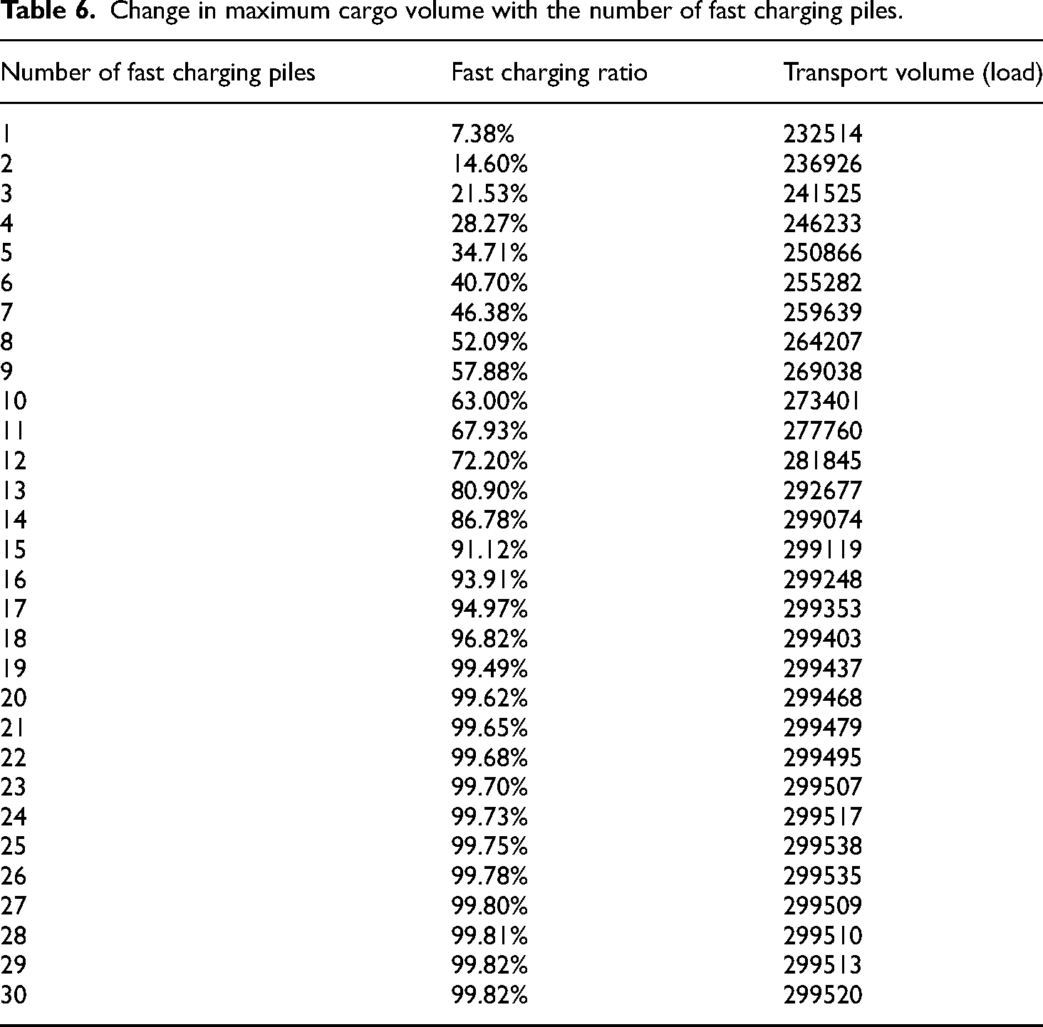
The optimal conditions are achieved when the number of fast charging piles reaches 14, and the fast-charging ratio reaches 86.78%. This is because, beyond this ratio, fast charging no longer significantly increases the total amount of goods transported.

After implementing the simulation scheduling algorithm, we developed a visual program to simulate the whole process. Figure 8 shows examples of the two scheduling processes. The specific scheduling process is given in Supplementary Materials.

Figure 8.

Simulation rendering.

This article provides Annexes III to VI, including executable algorithm scripts, visualization scripts, data attachments, and dynamic videos, for readers’ reference.

Conclusion

Previous research on unmanned vehicles has mostly focused on the operation control of the vehicles, with relatively little research on the scheduling of unmanned vehicles in specific environments. This study is the first to conduct mathematical modeling research on a bidirectional single-lane highway transportation system consisting of unmanned vehicles. We have designed efficient algorithms for solving the specified problem and achieved good results.

In this paper, the optimization of the scheduling scheme was solved by establishing a dynamic programming model to simulate the transportation and charging process of unmanned electric vehicles, and then solving the model through an algorithm to optimize the scheduling scheme. Finally, the simulation results were visualized and verified. The advantages of the proposed method are as follows:

The highly integrated optimization theory and algorithm achieves high efficiency with no need for intelligent optimization. Solutions are output in a short time, allowing the real-time scheduling of large workloads.

The simulation results can be directly visualized, making it easy to test the validity of the model and the accuracy of the results.

The model has strong universality. Changing parameters such as the total number of vehicles, total number of batteries, road length, and vehicle speed does not affect the solution efficiency.

One disadvantage of the proposed method is that the vehicle distance is fixed. This model fixes the position of the vehicles on the road section. This means that vehicle faults will be difficult to deal with. Associated problems could be avoided by increasing the estimated distance.

The main conclusions of this paper are as follows:

For the scheduling of self-driving electric vehicles, an optimization model has been established, and a simulation algorithm was developed to solve the optimization scheduling scheme. The algorithm effectively realizes the optimal scheduling scheme with extremely high operation efficiency. One prominent advantage is that the feasibility of the model can be tested very intuitively. Through the visualization function, the output results are transformed into the scheduling process to realize real-time testing of the scheduling scheme. This research can be extended to all applied mathematical problems that are difficult to solve based solely on theoretical derivation.

Supplemental Material

sj-docx-1-sci-10.1177_00368504231188617 - Supplemental material for Optimization of scheduling scheme for self-driving vehicles by simulation algorithm

Supplemental material, sj-docx-1-sci-10.1177_00368504231188617 for Optimization of scheduling scheme for self-driving vehicles by simulation algorithm by Xu Jianqiao in Science Progress

Supplemental Material

sj-docx-2-sci-10.1177_00368504231188617 - Supplemental material for Optimization of scheduling scheme for self-driving vehicles by simulation algorithm

Supplemental material, sj-docx-2-sci-10.1177_00368504231188617 for Optimization of scheduling scheme for self-driving vehicles by simulation algorithm by Xu Jianqiao in Science Progress

Supplemental Material

sj-docx-3-sci-10.1177_00368504231188617 - Supplemental material for Optimization of scheduling scheme for self-driving vehicles by simulation algorithm

Supplemental material, sj-docx-3-sci-10.1177_00368504231188617 for Optimization of scheduling scheme for self-driving vehicles by simulation algorithm by Xu Jianqiao in Science Progress

Supplemental Material

sj-docx-4-sci-10.1177_00368504231188617 - Supplemental material for Optimization of scheduling scheme for self-driving vehicles by simulation algorithm

Supplemental material, sj-docx-4-sci-10.1177_00368504231188617 for Optimization of scheduling scheme for self-driving vehicles by simulation algorithm by Xu Jianqiao in Science Progress

Footnotes

Declaration of conflicting interests

The author declared no potential conflicts of interest with respect to the research, authorship, and/or publication of this article.

Funding

The author(s) received no financial support for the research, authorship, and/or publication of this article.

ORCID iD

Xu Jianqiao

Supplemental material

Supplemental material for this article is available online.

Author biography

Xu Jianqiao, male, born in Wuxi, Jiangsu Province, is an undergraduate student of Nanjing University of Traditional Chinese Medicine. His main research directions are mathematical modeling, applied mathematics, and intelligent optimization algorithms. He is the first author of a paper related to mathematical modeling and intelligent algorithm application published in Scientific Reports.

References

Hong

Guo

Wang

, et al. The integrated scheduling optimization for container handling by using driverless electric truck in automated container terminal. Sustainability 2023; 15: 5536.

Zhang

de La Fortelle

, et al. State-driven priority scheduling mechanisms for driverless vehicles approaching intersections. IEEE Trans Intell Transp Syst 2015; 16: 2487–2500.

Liu

Cheng

Shi

, et al. A two-stage approach with a departure time based solution representation for electric bus vehicle scheduling. IEEE Access 2022; 10: 112799–112811.

Odili

. Combinatorial optimization in science and engineering. Curr Sci 2017; 113: 2268–2274.

Wang

Shi

Zuo

. A multi-objective genetic algorithm based approach for dynamical bus vehicles scheduling under traffic congestion. Swarm Evol Comput 2020; 54: 100667.

Shui

Zuo

Chen

, et al. A clonal selection algorithm for urban bus vehicle scheduling. Appl Soft Comput 2015; 36: 36–44.

Sowmya

Sankaranarayanan

. Optimal vehicle-to-grid and grid-to-vehicle scheduling strategy with uncertainty management using improved marine predator algorithm. Comput Electr Eng 2022; 100: 107949.

Fan

. Development and future trend of computer simulation and quantum computer simulation. J Syst Simul 2017; 29: 1161–1167.

Burger

Emer

Hoe

, et al. The future of architectural simulation. IEEE Micro 2010; 30: 8–18.

10.

Egonsdotter

Israelsson

. Computer-based simulations in social work education: a scoping review. Res Soc Work Pract 2022; 0.

11.

Chen

, et al. Computer simulations of surfactants and surfactant/polymer assemblies. Comput Mater Sci 2006; 36(4): 386–396.

12.

Linton

Sibly

Calow

. Testing life-cycle theory by computer simulation–I. Introduction of genetical structure. Comput Biol Med 1991; 21: 345–355.

13.

Rokosz

Hryniewicz

Malorny

, et al. ANSYS Analysis of stress and strain after cones plastic deformation. Tehnicki Vjesnik-Technical Gazette 2015; 22: 503–508.

14.

Malysza

Zuczek

Wilk-Kolodziejczyk

, et al. Technological optimization of the stirrup casting process with the use of computer simulations. Materials (Basel) 2022; 15: 6781.

15.

Durgut

Ayvaz

. A novel fully hybrid simulation-optimization approach for enhancing the calibration and verification performance of the TUW hydrological model. J Hydrol 2023; 617: 128976.

16.

Kenett

Vicario

. Challenges and opportunities in simulations and computer experiments in industrial statistics: an industry 4.0 perspective. Adv Theory Simul 2021; 4: 2000254.

17.

Liu

Mao

Song

, et al. Operation model design of two-way single lane bus lane system. Shanxi Jianzhu 2013; 039: 16–18.

18.

Liu

Yuan

. Research on vehicle lane-changing rules of two-way two-lane traffic flow model. Gansu Sci J 2012; 24: 5.

19.

Yang

. Multi-objective steel plate cutting optimization problem based on real number coding genetic algorithm. Sci Rep 2022; 12: 22472.

Supplementary Material

Please find the following supplemental material available below.

For Open Access articles published under a Creative Commons License, all supplemental material carries the same license as the article it is associated with.

For non-Open Access articles published, all supplemental material carries a non-exclusive license, and permission requests for re-use of supplemental material or any part of supplemental material shall be sent directly to the copyright owner as specified in the copyright notice associated with the article.

0.00 MB

0.02 MB

0.04 MB

0.02 MB