
Abstract
For evaluating the significance of renewable alternative fuels for optimized engine performance and lower emissions, methanol has been extensively utilized as a blend with gasoline in spark-ignition engines. However, rare attempts have been rendered to examine the consequence of methanol–gasoline fuel blends (M6, M12, and M18) on lubricant oil operating for a longer period in engines. The highest and least decrease of 9.62% and 6.68% in kinematic viscosity (KV) was observed for M0 and M18, respectively. However, the flash point (FP) of degraded lubricant oil for M6, M12, and M18 was 3%, 5%, and 7% higher than that of M0, respectively. Total acid number (TAN) and ash content of degraded lubricant oil for M18 were the highest among M0, M6, and M12. An inclusive optimization of engine performance, emissions, and lubricant oil properties has been made for various methanol–gasoline fuel blends at distinct operating conditions by employing the response surface methodology (RSM) technique. RSM-based optimization portrayed the composite desirability value of 0.73 for 2137.13 watt brake power (BP), 6.08 N-m torque, 0.37 kg/kwh brake-specific fuel consumption, 22.10% brake thermal efficiency, 4.02% carbon monoxide emission, 7.15% carbon dioxide emission, 134.12 ppm hydrocarbon emission, 517.02 ppm nitrogen oxides emission, 12.44 cst KV, 203.77°C FP, 2.23 mg/g KOH TAN, and 2.65%wt ash content as responses for fuel blend M8 at 3400 rpm and higher loading condition. RSM predicted results demonstrated significant compliance with empirical findings, with absolute percentage error (APE) below 5% for each response. However, the highest APE of 4.68% was obtained for FP owing to inefficient desirability as a consequence of manual testing. The least APE of 1.57% was obtained for torque because of the highest desirability. Overall, the RSM predicted results of the designed models are effective and viable. RSM technique was found to be effective for the optimization of the broader engine characteristics spectrum.
Introduction
The efforts of the modern world are focused on fuel conservation, optimization of engine performance, and exploration of alternatives to fossil fuels. Recently, many advancements have taken place to modify engine design, fuel properties, and emission abatement techniques. The energy demand of any country determines its socioeconomic growth. The number of people worldwide has increased considerably in previous years, reaching about 7.5 billion in 2017. 1 Immense growth in population over the past two decades, industrial development, and the quest to live luxurious life majorly contribute to the increase in fossil fuel utilization. 2 The major challenge is the depletion of fossil fuels due to augmented fuel consumption, strictness in emission regulations with every passing day, and hike in their prices which canvassed the significance of eco-friendly alternate fuels. 3 Tremendous research has already been done to estimate the remaining lifespan of these fossil fuel reserves and alarming results revealed the exhaustion of these reserves in the next 40 years. 4 Many factors like fuel demand, environment, economy, and geopolitical scenario influence the oscillation in price of fossil fuels. 5 Increased consumption of fossil fuel put adverse effects on climate like global warming, abrupt weather change, acid rain, cardiac and respiratory diseases, exhaustion of fuel reserves, smog, and diminution of ozone layers.6,7 The shifting trend toward alternative fuels significantly declines imports, balances the payments, improve environmental sustainability, create jobs, and boost exploration of indigenous renewable and hidden resources.8,9
The worldwide energy demand in just commercial transportation is projected to rise by 70% during 2010 to 2040, out of which 60% of this rise will affect heavy duty segment alone. 10 Ninety percent of the transport sector approximately rely on fossil fuels to provide power to engines. 11 Gasoline is gifted with a higher calorific value so that more energy could be extracted from gasoline in comparison with other alternatives to gasoline. The immense consumption of fossil fuel is not only accountable for its depletion but it is also accountable for global warming and polluted environment. 8 In the consideration of the electrification of motor transport sectors, current electricity generation capacity will not be enough to deliver a complete electrical worldwide foot. The creation of environmental concerns is not unlikely for electric automobiles. The establishment of appropriate alternative fuels for the existing vehicle motors is, therefore, highly vital for reducing the fossil fuel consumption and environmental contamination for further 10–20 years.12–14 Methanol served as an attractive alternative to gasoline because of naturally optimized properties. The lesser refining operations required in the case of methanol is mainly responsible for its lower price in comparison with gasoline. The production cost of methanol is 350 USD/ton in China, approximately half from the petroleum fuels. 15 The estimated production cost of methanol is still lower than gasoline even in terms of equivalence energy. Also, the production cost of methanol is about 50% lower than the cost of petroleum fuels in Canada. 16 The appropriate fuel combustion owing to lower boiling point of methanol is mainly responsible for lower emissions from methanol blended fuels. The higher oxygen proportion (50% by weight) in methanol increased octane rating, flammability limit, and laminar flame speed along with lower carbon-to-hydrogen ratio which mainly result in lower carbon monoxide emissions.15,17 Furthermore, methanol exhibits higher latent heat of vaporization and lower vapor pressure which restrict its utilization as a fuel in automotive owing to cold start issues. Different techniques like fuel reforming, blend fuels, intake air, and fuel heating have been incorporated in order to utilize methanol effectively as an alternative for fossil fuel. 18 Methanol exhibits three to five times higher latent heat of vaporization as compared to gasoline; this characteristic is primarily accountable for higher volumetric efficiency. The fuel with the higher latent heat of vaporization lowers the temperature of the intake manifold through cooling of the incoming mixture to a dense mixture and ultimately result in higher power output. 19 In this regard, alcohols are used as additives to modify fuel properties and optimize engine performance. 20 The fuel blends having different proportions of methanol in gasoline fuel allow spark Ignition (SI) engine to run at augmented compression ratios without any knocking owing to higher octane number.
Literature survey
Mallikarjun and Mamilla 21 examined the impact of 3% to 15% methanol blends under different load settings. They observed higher brake thermal efficiency (BTE), CO2, and NOx besides decline in carbon monoxide (CO) and hydrocarbon (HC) emissions. Shayan et al. 22 recorded exhaust emissions for methanol–gasoline fuel blends. They monitored decline in average HC (24.9%) and CO (23.7%) emissions, respectively. However, increase of 7.5% and 17.5% was observed for CO2 and NOx, respectively, in contrast to gasoline. Altun et, al. 23 evaluated impact of M10 and attained 13 and 10.6% lower HC and CO emission respectively. Ahmed et al. 24 employed various methanol blends in single-cylinder SI engine ranging from 0% to 18% with equal intervals of 3%. They perceived percentage rise in the NOx emissions were 5.49, 12.54, 19.19, 28.73, 35.81, and 41.13 for M3, M6, M9, M12, M15, and M18, respectively. The percentage decline in HC emissions was 2.12, 4.97, 7.92, 11.05, 14.14, and 17.04. The percentage decrease in the CO emissions was 4.66, 10.19, 15.17, 19.36, 23.87, and 29.05. The percentage decrease in the CO2 emissions were 2.23%, 5.05%, 6.65%, 11.18%, 14.07%, and 16.84%. The percentage increase in torque was 5.62, 6.83, 7.28, 10.02, 6.73, and 2.73. The percentage increase in brake power (BP) was 5.62, 6.83, 7.28, 10.02, 6.73, and 2.73. The average BTE was 17.36, 18.33 18.96, 19.66, 20.03, 19.35, and 18.47%. While, the average brake specific fuel consumption (BSFC) was 0.458, 0.447, 0.438, 0.430, 0.428, 0.450, and 0.481 kg/kWh. Abu-Zaid et al. 25 achieved the finest results for M15 which comprised of higher power output and lower BSFC. Elfasakhany 6 performed experiment on carburetor type unmodified SI engine under wide open throttle setting to check the performance of various lower concentrated methanol blended gasoline fuels (M3, M7, and M10). The experimental results revealed that BP for M3, M7, and M10 increased by 1.23%, 0.53%, and 0.82%, respectively, at 3200 rpm. The torque for M3, M7, and M10 increased by 1.29%, 0.43% and 0.86% respectively at 3200 rpm. Similarly, the BP for M3, M7, and M10 increased by 2.13%, 2.55%, and 2.55%, respectively, at 2700 rpm. The torque for M3, M7, and M10 augmented by 2.41%, 1.32%, and 1.32%, respectively, at 2700 rpm. Farkade and Pathre 26 disclosed the increase in NOx for methanol mixed fuel in contrast to gasoline was because of higher oxygen proportion and adiabatic flame temperature.
The present work highlights the importance of lubricant oil in engine which is the main characteristic of tribology. Lubricants capable of forming low-strength sheared induced tribofilms and reducing the interfacial contact area at a given normal load will improve tribological system lubricity during sliding. Lubricants have long been regarded as an effective means of reducing friction and protecting wear in mechanical systems that flows everywhere inside an engine and significantly affects the engine performance. The lubrication in automotive is characterized into mixed regime, boundary regime, and elastohydrodynamic regime. 27 Different lubrication regimes, depending upon the running conditions, during one stroke can occur throughout the stroke. The mixed or boundary lubrication regimes occur at start and end of the stroke while hydrodynamic lubrication regime occurs at middle of the stroke. 28 Consequently, hydrodynamic friction rises because of the prevailing circumstances of low loading and elevated speeds. 29 The piston ring assembly at the top dead center and bottom dead center, asperity contact location, comprises totally of viscous and boundary friction owing to the shearing of lubricant. The boundary lubrication takes place for only thin oil films. The load is not carried out by lubrication film but instead it is maintained on surface peaks. 30 It is assessed that frictional losses of up to 30% occur at piston ring assembly, emphasizing on the importance of tribological performance. 31 The deterioration of lubricant oil is unavoidable but it should be prolonged through performance additives. During engine operations, oxidation, contamination, and thermal cracking of lubricant oil performs a substantial role in the lube oil degradation which may affect its chemical reactivity through acid or base formation, variation in thermal conductivity, and viscosity. Gulzar et al. 32 employed lubricant oil of grade 15W40 in single-cylinder diesel engine and operated engine on neat diesel, 20% palm biodiesel (PB20), and 20% jatropha biodiesel (JB20). They observed general declining trend in lubricant oil viscosity for all three fuels due to fuel dilution in lubricant oil with time. More decline in the viscosity was observed for biodiesel fuels. The general increasing trend of lubricant oil density was observed. However, the lubricant oil utilized for biodiesel exhibited higher density due to contamination and wear debris. Total acid number (TAN) usually increases with time due to corrosion and oxidation. The higher TAN value for oil samples that operated on B20 was responsible for higher corrosion rate and quicker oxidation which decreases life of the lubricant oil during engine endurance tests. Usman and Hayat 33 used 125cc motorbike engine to examine the impact of liquified petroleum gas (LPG) and gasoline on emissions, performance, and lubricant oil deterioration. They observed a reduction of 17.4% and 10% in BP and torque, respectively, for LPG in contrast to gasoline when fresh lubricant oil was used. Reduction of 21% and 10.6% in BP and torque, respectively, was observed in the case of deteriorated lubricant oil. TAN was increased by 65.2% and 21.7% for gasoline and LPG, respectively. Flash point (FP) and ash contents were decreased by 16% and 8.69% for gasoline, respectively, but they were augmented by 1.66% and 44.5% in the case of LPG. Kinematic viscosity (KV) is declined for both the fuels. Hasannuddin et al. 34 employed emulsion fuels in a 400cc diesel engine and made comparison by evaluating the effect of emulsion fuel and diesel on lubricant oil. They observed lower wear rate inside engine cylinder when emulsion fuels were used. Iron (Fe), aluminum (Al), copper (Cu), and lead (Pb) wear debris concentrations were declined by 8.2%, 9.1%, 16.3%, and 21.0%, respectively, for emulsion fuel in contrast to diesel. The FP and viscosity of lubricant oil operated on the emulsion fuel is raised by 2% and 14.31% in contrast to diesel fuel. The ash content and TAN in lubricant oil is declined by 4.40% and 18% for emulsion fuel. Usman and Hayat 35 used a 219cc single-cylinder engine to record lubricant oil deterioration in the case of compressed natural gas (CNG) and gasoline. They investigated wear debris (Fe, Al, Cu, and chromium (Cr)),lubrication oil condition (KV, FP, and total base number (TBN)), and additives depletion (zinc and calcium). The testing of lubricant oil depicted 4.9%, 9.5%, and 3.2% higher KV, FP, and TBN for CNG respectively as compared to lubricant oil ran on gasoline. Therefore, Fe, Cu, Al, and Cr is declined by 13.8%, 37.7%, 29.1%, and 30% in the case of CNG, respectively. The zinc diminution was monitored at higher load for gasoline (0.11%wt) and CNG (0.12%wt). A drastic decrease in calcium was observed for gasoline (0.2127%wt) in comparison with CNG (0.2377%wt).
Response surface methodology (RSM) is a technique which provides optimized solutions to a variety of industrial problems. 36 It provides efficient and cost-effective solutions for assessing experimental variables. 37 The RSM analysis proposes optimized data sets with the best system performance and saves both time and money. 38 This method has been applied in numerous studies for optimizing engine efficiency. 39 Najafi et al. 40 evaluated engine performance and emissions with main objective to determine ideal conditions for improved efficiency and lower emissions. The optimum values were determined at a 3000 rpm engine speed for 10% bioethanol–gasoline blend. The performance responses were achieved as BP (35.26 kW), torque (103.66 Nm), BSFC (0.25 kg/kWh), CO (3.5%), CO2 (12.8%), HC (136.6 ppm), and NOx (1300 ppm). The performance of a SI engine employing various fuel oil blends (0%, 25%, 50%, 75%, and 100%) under distinct loading conditions (20%, 40%, 60%, 80%, and 100%) at fixed 2500 rpm were investigated using RSM by Ardebili. 41 The optimization results advised engine load of 47.21% and fuel oil level of 25%. The torque (16.49 Nm), BSFC (326.02 g/KWh), CO (0.88%), NOx (568.3 ppm), and HC (165.49 ppm) were recorded at these optimal operating conditions. BTE and torque declined along with drastically lower in-cylinder temperatures. NOx emissions decreased by 41% when fuel oil content was increased from 20% to 100%, whereas HC and CO emissions were augmented by 39% and 22%, respectively. RSM was effectively utilized for the modeling and optimization of engine performance parameters, as evidenced by a higher desirability value of about 0.63 in the regression model.
The detailed study of literature revealed that the lubricant oil deteriorated by gasoline, LPG, CNG, diesel, biodiesel, and emulsion fuels has been substantially investigated. However, no serious attempt has been made to ascertain the effect of methanol–gasoline fuel blends on the degradation of lubricant oil along with environmental emissions and engine performance. Consequently, this study involves investigation of the very novel issue. The functioning temperature and physicochemical traits of methanol mixed fuels are not analogous to pure gasoline fuel. This highlights the substantial difference of lubricant oil degradation inside a SI engine when fueled with methanol–gasoline blends and gasoline for 120 h of engine operations.
After empirical findings, the novel optimization of all three aspects including engine performance, emissions, and lubricant oil deterioration is made through RSM approach. A multilevel historical design is applied through Design Expert software for the optimization of all parameters. The design is formed by user-defined discrete levels. Fuel blend, engine speed, and load are the input factors with four levels (M0, M6, M12, and M18), seven levels (2800, 2900, 3000, 3100, 3200, 3300, and 3400 rpm), and two levels (20 and 40 psi), respectively. The BP, torque, BSFC, BTE, CO, CO2, HC, NOX, KV, FP, TAN, and ash content are the response variables of RSM model. RSM is employed for evaluating the individual interactions between input and response variables along with statistical significance of developed models. The finest fit model for every response is opted and analysis of variance (ANOVA) is applied for better understanding of model characteristics. Finally, the experiment was again performed only on optimized conditions specified by RSM in order to validate its authenticity of prediction.
Methodology
The current experimental study involves investigation of gasoline engine (model: HONDA GP160, 163cc, four strokes and air cooled with overhead valves) to determine its performance, emissions, and lubricant oil degradation when charged with different methanol–gasoline fuel blends. The comprehensive technical specifications of an engine are shown in Table 1.
Engine technical specifications.

Materials
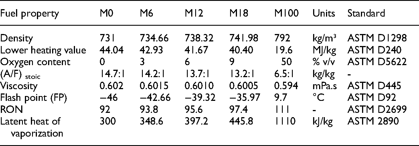
Base gasoline (M0) was procured from Pakistan State Oil. Methanol was procured from Merck chemicals. Both gasoline and methanol were mixed in accordance to percentage by volume to give various proportions like 6% methanol mixed in 94% gasoline (M6), 12% methanol blended in 88% gasoline (M12), and 18% methanol blended in 82% gasoline (M18), with the aim to ascertain the emission attributes and performance of gasoline engine as well as the deterioration of the lubricant oil. Both gasoline and methanol were first mixed in the measuring cylinder with respect to their percentage volume in blended fuel, and then the mixture was stirred continuously through magnetic stirrer (hot plate model 78-1) for a period of 30 min in order to assure the homogenous mixture of fuels. The four test fuels (M0, M6, M12, and M18) were added into the test engine intake manifold through a transparent measuring cylinder of capacity 500 ml with least count of 1 ml in order to calculate fuel flow rate. Table 2 presents the physicochemical properties of four test samples with different blend ratios of methanol in gasoline. Table 3 shows the attributes of lubricant oil (SAE 20W-40), and this certain lube oil grade was used in the engine according to engine manufacturer's recommendation.
Physicochemical characteristics of test fuels.
Physicochemical attributes of fresh lubricant oil sample.

TAN: total acid number.
Experimental arrangement
HONDA GP-160 (SI engine) was attached with 7-inch kart, water brake dynamometer of DYNOMITE company in order to ascertain engine performance. Figure 1 shows experimental arrangement of all instruments which coupled with an engine to ascertain the results. Figure 2 shows the actual experimental test bench. DYNO-MAX 2010 software was dedicated for operating and displaying all engine parameters. The sensors in the dynamometer, transmitted signals to the data acquisition system, in order to record the engine speed (rpm) and torque. The engine operated at different speeds range from 2800 rpm to 3400 rpm, and loads (lower load of 20 psi water pressure and higher load of 40 psi of water pressure) were applied. The applied load change was achieved by water pump of 1 horse power linked with dynamometer, that is, water was supplied to dynamometer's housing via load control valve and water whipped around toroidal pockets inside the housing which were driven by an engine. The shear forces produced in the water act as a load on the engine by opposing the motion of the engine shaft as directed peripheral to housing radius of shaft. The probe of exhaust gas analyzer (EGA) modeled as EMS-5002 was inducted into tail pipe of engine for the measurement of emissions. The K type thermocouple was attached to engine for monitoring the engine temperature for its operations within the safe limit.
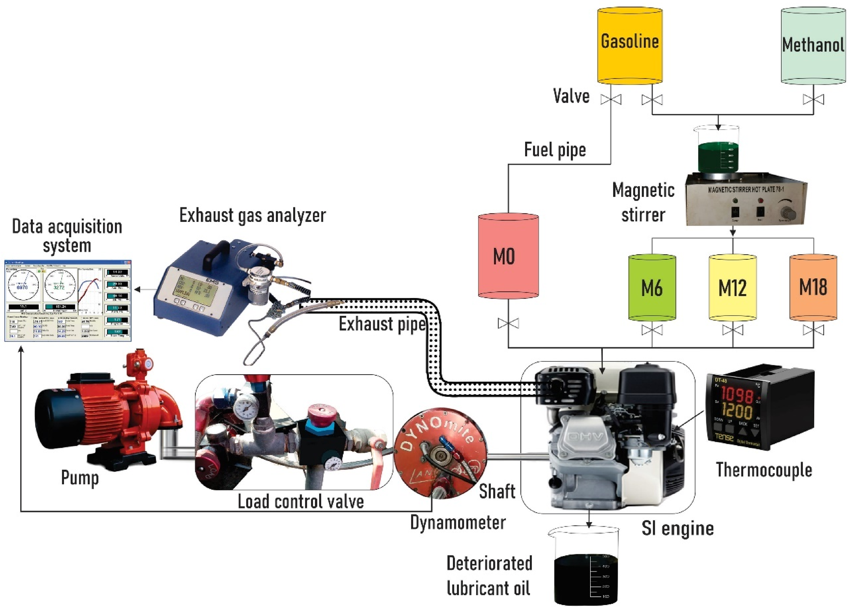
Experimental setup.

Engine on experimental test bench.
Test approach
The testing scheme was adopted to assess the engine performance and emissions, as well as condition monitoring strategies and sampling method for lube oil as shown in Table 4. Before beginning the experiment, the engine seals were examined for leaks and fresh air filters were employed to ensure proper air flow to the engine. With reference to gasoline, the comparison is made on how these methanol–gasoline fuel blends impact engine performance (BP, torque, BSFC, and BTE), emissions (CO, CO2, HC, and NOx), and lubricant oil condition. The brake power and torque were ascertained through dynamometer from speed range between 2800 rpm and 3400 rpm and load range between 20 psi and 40 psi. For a time period of 1 min at a certain rpm, a probe of EGA was inducted in tail pipe to attain steady-state emissions (HC (ppm), NOx (ppm), CO (%), and CO2 (%)). Hence, torque, fuel consumption, and emissions were noted against applied loads and respective speeds.
Brief of engine testing plan.

Furthermore, lube oil was withdrawn from the engine after 120 h of engine running at specified speed and load in order to investigate its physicochemical properties. The engine was first run for 120 h on M0, after which the lubricant oil was removed and tested for its physicochemical properties. Likewise, the same procedure adopted for M6, M12, and M18 in order to test the variation in their physicochemical traits. The deterioration rate of lube oil is calculated by comparing the variance in attributes of lube oil that is operated on test fuels (M0, M6, M12, and M18) subsequently in contrast to fresh lubricant oil as a baseline. Table 3 mentions physicochemical attributes of fresh lubricant oil. Then, the emissions, engine performance along with lubricant oil degradation data was imported to Design Expert software in order to implement RSM technique. 3D surface view plots and comparison between actual and predicted values were developed depending on independent factors (fuel blend, load, and speed). An empirical model was best fitted and ANOVA was used to examine the association among variables and responses. At last, the multi-objective optimization was obtained by employing desirability function. The RSM optimized results was then validated through experimentation.
Results and discussion
Four test fuels (M0, M6, M12, and M18) were employed in 163cc, air-cooled, four-stroke SI engine to evaluate the lubricant oil degradation, emissions, and performance parameters. Then, these engine operating parameters were optimized and validated through RSM technique. The comprehensive analysis on these aspects is stated below.
Impact on engine performance
The BP, torque, BSFC, and BTE are ascertained as engine performance parameters and optimized through RSM technique.
BP
BP possesses a direct relationship with engine speed and torque. Figure 3(a) shows the trend of BP for various methanol–gasoline fuel blends from speed ranging between 2800 rpm and 3400 rpm for lower load. As the concentration of methanol rises in the gasoline blend, the BP also augments but after certain percentage of methanol in gasoline blends, the BP starts to decline. The BP in the case of M6 and M12 under lower load settings was 8.34% and 17.30% higher than that of M0, respectively, while for M18, it was 3.67% lower than that of M0 at lower load. The marginally lower BP in the case of M18 can be credited due to lower calorific value of methanol in contrast to gasoline. 24 Figure 3(b) indicates the trend of BP for test fuels range from M0 to M18 with gap of 6% methanol concentration in gasoline blend and speed ranging between 2800 rpm and 3400 rpm for higher load. The BP for M6, M12, and M18 at higher load was 6.84%, 8.85%, and 0.87% higher than that of M0, respectively. Figure 3(a) and 3(b) show higher brake power in the case of all fuels under higher load as compared to fuels under lower loading condition. M0, M6, M12, and M18 produced 35.75%, 33.88%, 25.97%, and 42.16% higher BP at higher load in comparison with lower load, respectively.

Comparison of brake power (BP) (a) at lower load, (b) at higher load, and (c) between actual and predicted values.
The comparison between actual and RSM predicted BP is presented in Figure 3(c). The color points from blue to red color represent the minimum BP of 1023.27 watt and maximum BP of 2238.78 watt, respectively. Table 5 signifies ANOVA for reduced quadratic model in the case of BP. The probability distribution with F and p-values of 112.02 and smaller than, 0.05 respectively, indicates greater statistical significance of measured BP. Moreover, the quadratic regression model appeared to be a perfect fit with data points in close proximity with regression line. It indicates the minimum possible deviations between predicted and actual data set values.
Analysis of variance (ANOVA) for reduced quadratic model in the case of brake power (BP).

The p-values from Table 5 show that all three factors including speed, load, and fuel blends are significant. Moreover, the R2 value of 0.97 was close to positive unity and there was sufficient agreement between predicted and adjusted R2. The predicted R² of 0.95 was in fair compliance with adjusted R² of 0.96; that is the difference in between them was equivalent to 0.01. The speed and load were significantly contributed to aggregated variations with PC% of 52.5% and 40.7%, respectively, in comparison with fuel blend which was 2.86%. Despite of apparently efficient prediction capacity of the model validated by graphs and statistical parameters, its results may be misleading owing to the doubt that there could be some other model with more promising fit for available data, that is, lack of fit is present in data. This issue has been addressed with the lack of fit (F-test) performed with the significance level of 0.01. The hypothesis testing was centered around:
F0: The assumed relation is reasonable, that is, there is no lack of fit. F1: The relation assumed is not reasonable, that is, there is a lack of fit present in the model.
For accepting or rejecting the null hypothesis (F0), the calculated p-value was used a reference. For the case of the BP, the p-value given by design expert is less than 0.01, which is testimonial to fact that we fail to reject null hypothesis and do not have enough evidence to prove the presence of lack of fit in the reduced quadratic model. The best fitted quadratic model from the fit summary was selected due to aliased nature and poor fit of cubic and linear models, respectively. The actual BP regression equation is shown in equation (1):
Torque
Figure 4(a) specifies the trend of torque for various methanol–gasoline fuel blends at lower load setting. The torque augmented with the rise of methanol concentration in gasoline. However, after certain proportion of methanol in gasoline blend, the torque declined. The torque for M6 and M12 under lower load setting was 8.33% and 17.12% higher than that of M0, respectively, while for M18, it was 3.74% lower than that of M0 at lower load. The marginally lower torque in the case of M18 can be credited due to lower calorific value of methanol in contrast to gasoline. 24 Figure 4(b) indicates the trend of torque for test fuels range from M0 to M18 with gap of 6% methanol concentration in gasoline blend at higher load setting. The torque for M6, M12, and M18 at higher load was 7.05%, 8.64%, and 0.85% higher than that of M0, respectively. It is apparent from Figure 4(a) and 4(b) that higher torque produced by all the fuels at higher load in comparison with fuels which burned at lower load. The M0, M6, M12, and M18 produced 35.88%, 34.27%, 26.03%, and 42.35% higher torque at higher load in comparison with lower load, respectively. The overall growing trend of torque with the progression in speed and load can be credited due to the faster burning of fuel to fulfill high power needs. 19 The augmented torque for methanol blends due to improved combustion, elevated oxygen proportion, and quicker promulgation of laminar flame.45–47 The naturally higher octane rating of methanol is responsible for reduced knocking and advanced injection timing which mainly result higher cylinder pressure and torque. 6

Comparison of torque (a) at lower load, (b) at higher load, and (c) between actual and predicted values.
The comparison between actual and RSM predicted torque is presented in Figure 4(c). The color points from blue to red color represent the minimum torque of 3.49 N-m and maximum torque of 6.29 N-m, respectively. Table 6 signifies ANOVA for reduced quadratic model in the case of torque. Moreover, the quadratic regression model appeared to be a perfect fit with data points in close proximity with regression line. It indicates the minimum possible deviations between predicted and actual data set values.
Analysis of variance (ANOVA) for reduced quadratic model in the case of torque.

The probability distribution with F and p-values of 93.21 and smaller than 0.05, respectively, indicates greater statistical significance of measured torque. The p-values from Table 6 show that all three factors including speed, load, and fuel blends are significant. Moreover, the R2 value of 0.97 was close to positive unity and there was sufficient agreement between predicted and adjusted R2. The predicted R² of 0.94 was in fair compliance with adjusted R² of 0.96; that is, the difference in between them was equivalent to 0.02. The speed and load were significantly contributed to aggregated variations with PC% of 16.4 and 72.8%, respectively, in comparison with fuel blend which was 5.11%. For the case of the torque, the p-value given by design expert is less than 0.05, which is testimonial to the fact that we fail to reject null hypothesis and do not have enough evidence to prove the presence of lack of fit in the reduced quadratic model. The best fitted quadratic model from the fit summary was selected due to aliased nature and poor fit of cubic and linear models, respectively. The actual torque regression equation is shown in equation (2):
BSFC
The variation in the trend of BSFC for various methanol–gasoline fuel blends at lower load setting is shown in Figure 5(a). The methanol–gasoline fuel blends show slightly higher BSFC in comparison with gasoline mainly due to lower calorific value and higher fuel-to-air ratio of methanol.25,48 The lowest BSFC at 2800 rpm and lower load indicates highest fuel conversion efficiency. The BSFC for M6 and M18 at lower load was 0.79% and 15.16% higher than that of M0, respectively, while for M12, it was 1.10% lower than that of M0 at lower load. Figure 5(b) indicates the trend of BSFC for test fuels range from M0 to M18 with gap of 6% methanol concentration in gasoline blend at higher load setting. The fuel consumption gets lower at higher engine speeds due to higher cylinder pressure and fuel density which ultimately result into higher brake thermal efficiency.3,22 The BSFC for M18 at higher load was 2.33% higher than that of M0, respectively, while BSFC for M6 and M12 was 4.63% and 7.49% lower than that of M0 at higher load. The lower BSFC for leaner methanol blends can be reasoned to elevate the octane rating and volumetric efficiency of methanol. However, BSFC is greater for higher methanol–gasoline fuel blends due to lower calorific value of methanol. 49 The least BSFC for all test fuels was achieved at 2800 rpm under lower load settings and at 3400 rpm under higher load settings. The M0, M6, M12, and M18 demonstrated 16.07%, 17.28%, 19.66%, and 22.45% less BSFC at higher load in comparison with lower load, respectively. The greater power output at higher load generated lower BSFC.

Comparison of BSFC (a) at lower load, (b) at higher load, and (c) between actual and predicted values.
The comparison between actual and RSM predicted BSFC is presented in Figure 5(c). The color points from blue to red color represent the minimum BSFC of 0.36 kg/kwh and maximum BSFC of 0.56 kg/kwh, respectively. The minimal deviations of predicted values from the actual data sets are testimonial to a good fit of the quadratic regression model. The data points were in close proximity of regression line which indicated a good fit of the quadratic regression model. Table 7 signifies ANOVA for reduced quadratic model in the case of BSFC. Moreover, the quadratic regression model appeared to be a perfect fit with data points in close proximity with regression line. It indicates the minimum possible deviations between predicted and actual data set values.
Analysis of variance (ANOVA) for reduced quadratic model in the case of BSFC.

The probability distribution with F and p-values of 49.10 and smaller than 0.05, respectively, indicates greater statistical significance of measured BSFC. The p-values from Table 7 show that all three factors including speed, load, and fuel blends are significant. Moreover, the R2 value of 0.97 was close to positive unity and there was sufficient agreement between predicted and adjusted R2. The predicted R² of 0.91 was in fair compliance with the adjusted R² of 0.95; that is, the difference in between them was equivalent to 0.04. The fuel blend and load were significantly contributed to aggregated variations with PC% of 15.5% and 63.6%, respectively, in comparison with speed which was 0.22%. For the case of the BSFC, the p-value given by design expert is less than 0.05, which is testimonial to the fact that we fail to reject null hypothesis and do not have enough evidence to prove the presence of lack of fit in the reduced quadratic model. The best fitted quadratic model from the fit summary was selected due to aliased nature and poor fit of cubic and linear models, respectively. The aliased quadratic model not only allows the estimation of the influence of speed, load, and blend separately on BSFC, but also allows the interaction between input variables and investigation of their synergic effect on BSFC. The actual BSFC regression equation is shown ins equation (3):
BTE
The variation in the trend of BTE for various methanol–gasoline fuel blends at lower load setting is shown in Figure 6(a). BTE represents the effective conversion of fuel energy to BP. BTE was found higher at lower speed and lower loading condition due to the formation of lean mixture. The main reason for decreased BTE at higher speed is fast and abrupt combustion. 50 The average BTE of M0, M6, M12, and M18 at lower load was 17%, 18%, 19%, and 16%, respectively. The rise in BP and efficient burning for M6 and M12 fuel blends is accountable for higher BTE. The isochoric combustion and lower dissociation losses are responsible for increase in BTE. 51 However, the higher fuel consumption for M18 fuel is accountable for lower BTE. Figure 6(b) indicates the trend of BTE for test fuels range from M0 to M18 with gap of 6% methanol concentration in gasoline blend at higher load setting. The average BTE of M0, M6, M12, and M18 at higher load was 19%, 20%, 22%, and 21%, respectively. BTE exhibits inverse relationship with calorific value and BSFC, 52 therefore, reduction in heat dissipation boosts the BTE. The methanol possesses higher latent heat of evaporation which is responsible for more heat soaking up from the cylinder walls during compression. 53 Consequently, BTE increases due to lower work required for the compressing air–fuel mixture. The heat losses from cylinder walls are lower in the case of methanol due to quicker laminar flame speed and improved isometric effect. 46 M0, M6, M12, and M18 demonstrated 2%, 2%, 3%, and 5% higher BTE at higher load in comparison with lower load, respectively. The maximum BTE of 23.55% is demonstrated by M12 at higher load and at 3400 rpm.

Comparison of BTE (a) at lower load, (b) at higher load, and (c) between actual and predicted values.
The comparison between actual and RSM predicted BTE is presented in Figure 6(c). The color points from blue to red color represent the minimum BTE of 15.75% and maximum BTE of 23.67%, respectively. Table 8 represents the ANOVA for reduced quadratic model in the case of BTE. The probability distribution with F and p-values of 12.59 and smaller than 0.05, respectively, indicates greater statistical significance of measured BTE. Moreover, the quadratic regression model appeared to be a perfect fit with data points in close proximity with regression line. It indicates the minimum possible deviations between predicted and actual data set values.
Analysis of variance (ANOVA) for reduced quadratic model in the case of BTE.

The p-values from Table 8 show that all three factors including speed, load, and fuel blends are significant. Moreover, the R2 value of 0.86 was close to positive unity and there was sufficient agreement between predicted and adjusted R2. The predicted R² of 0.65 was in fair compliance with the adjusted R² of 0.79; that is, the difference in between them was equivalent to 0.14. The fuel blend and load are significantly contributed to aggregated variations with PC% of 3.61% and 57.1%, respectively, in comparison with speed which was 3.22%. For the case of the BTE, the

Impact on exhaust emissions
The CO, CO2, HC, and NOx are ascertained as emission characteristics of an engine and optimized through RSM technique.
The considerable decrement in CO emissions for various methanol–gasoline fuel blends in the speed ranging between 2800 rpm and 3400 rpm can be seen from Figure 7(a). The CO emission for M6, M12, and M18 was 8.68%, 18.62%, and 28.78% lower than that of M0, respectively, at lower load. It can be credited due to greater latent heat of evaporation of methanol which is accountable for amplified volumetric efficiency, greater molecular diffusivity, extra homogeneous mixing, greater flammability limit, and improved combustion for methanol mixed fuels. 54 Figure 7(b) indicates the trend of CO for the test fuels in the speed ranging between 2800 rpm and 3400 rpm under high load setting. The M6, M12, and M18 produced 22.18%, 26.16%, and 32.40% lower CO emission than that of M0, respectively, at higher load. The decrease of 20.32%, 32.10%, 27.70%, and 24.37% CO emissions for M0, M6, M12, and M18 was observed at higher load in contrast to lower load, respectively. The existence of oxygen in methanol is accountable for lower fuel-to-oxygen ratio which considerably raises the rich fuel zones in combustion chamber. 24 The lower carbon-to-hydrogen ratio of methanol is also responsible for lower CO emission. 55

Comparison of CO emission (a) at lower load, (b) at higher load, and (c) between actual and predicted values.
The comparison between actual and RSM predicted CO emission is presented in Figure 7(c). The color points from blue to red color represent the minimum CO emission of 2.01% and maximum CO emission of 5.42%, respectively. Table 9 signifies ANOVA for reduced quadratic model in the case of CO emission. Moreover, the quadratic regression model appeared to be a perfect fit with data points in close proximity with regression line. It indicates the minimum possible deviations between predicted and actual data set values.
Analysis of variance (ANOVA) for reduced quadratic model in the case of CO emission.

The probability distribution with F and p-values of 225.28 and smaller than 0.05, respectively, indicates greater statistical significance of measured CO emission. The p-values from Table 9 show that all three factors including speed, load, and fuel blends are significant. Moreover, the R2 value of 0.98 was close to positive unity and there was sufficient agreement between predicted and adjusted R2. The predicted R² of 0.97 was in fair compliance with adjusted R² of 0.98; that is, the difference in between them was equivalent to 0.01. The speed and load were significantly contributed to aggregated variations with PC% of 46.2% and 29%, respectively, in comparison with fuel blend which was 23.1%. For the case of the CO emission, the p-value given by design expert is less than 0.05, which is testimonial to the fact that we fail to reject null hypothesis and do not have enough evidence to prove the presence of lack of fit in the reduced quadratic model. The best fitted quadratic model from the fit summary was selected due to aliased nature and poor fit of cubic and linear models, respectively. The actual regression equation in the case of CO emission is shown in equation (5):
The variation in the trend of CO2 emissions for various methanol–gasoline fuel blends in the speed ranging between 2800 rpm and 3400 rpm is shown in Figure 8(a). The CO2 emission for M6, M12, and M18 was 3.83%, 8.42%, and 12.5% lower than that of M0, respectively, at lower load. The greater oxygen content and greater hydrogen-to-carbon ratio in methanol is responsible for decremented CO2 emissions for methanol blended fuels in contrast to gasoline. 56 Figure 8(b) indicates the trend of CO2 emission for the test fuels in the speed ranging between 2800 rpm and 3400 rpm at higher load. The M6, M12, and M18 produced 6.89%, 9.85%, and 14% lower CO2 emission than that of M0, respectively, at higher load. The decrease of 15.20%, 17.90%, 16.53%, and 16.65% CO2 emissions for M0, M6, M12, and M18 was observed at higher load in comparison with lower load, respectively.

Comparison of CO2 emission (a) at lower load, (b) at higher load, and (c) between actual and predicted values.
The comparison between actual and RSM predicted CO2 emission is presented in Figure 8(c). The color points from blue to red color represent the minimum CO2 emission of 5.11% and maximum CO2 emission of 8.51%, respectively. Table 10 signifies ANOVA for reduced quadratic model in the case of CO2 emission. Moreover, the quadratic regression model appeared to be a perfect fit with data points in close proximity with regression line. It indicates the minimum possible deviations between predicted and actual data set values.
Analysis of variance (ANOVA) for reduced quadratic model in the case of CO2 emission.
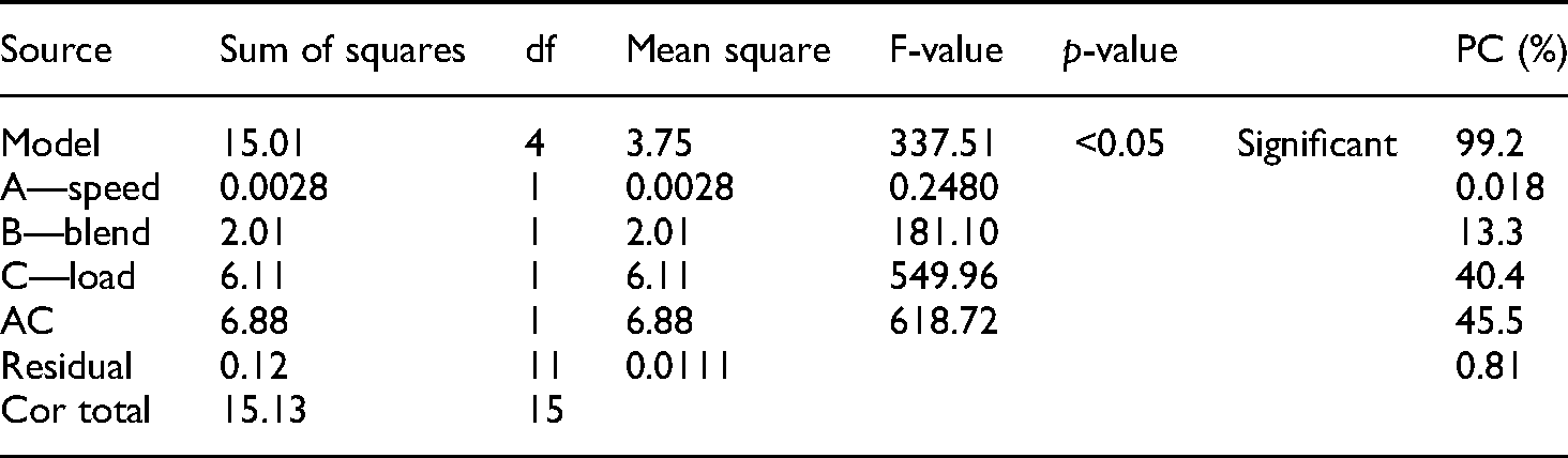
The probability distribution with F and p-values of 337.51 and smaller 0.05, respectively, indicates greater statistical significance of measured CO2 emission. The p-values from Table 10 show that all three factors including speed, load, and fuel blend are significant. Moreover, the R2 value of 0.99 was close to positive unity and there was sufficient agreement between predicted and adjusted R2. The predicted R² of 0.98 was in fair compliance with the adjusted R² of 0.99; that is, the difference in between them was equivalent to 0.01. The fuel blend and load were significantly contributed to aggregated variations with PC% of 13.3% and 40.4%, respectively, in comparison with speed which was 0.018%. For the case of the CO2 emission, the p-value given by design expert is less than 0.05, which is testimonial to the fact that we fail to reject null hypothesis and do not have enough evidence to prove the presence of lack of fit in the reduced quadratic model. The best fitted quadratic model from the fit summary was selected due to aliased nature and poor fit of cubic and linear models, respectively. The aliased quadratic model not only allows the estimation of the influence of speed, load, and blend separately on CO2 emission, but also allows the interaction between input variables and investigation of their synergic effect on CO2 emission. The actual regression equation in the case of CO2 emission is shown in equation (6):

Equation (6) indicates the impact of each independent variable on the response for specified levels of each factor in terms of original units.
HC emission is the result of unburned fuel vaporization and inadequate fuel burning. The primary causes of HC emission are leakage from fuel valves, state of fuel during engine warm up and cold start, deposition of unburned fuel in cracks, and engine misfire. 57 Furthermore, lower ignition energy, more homogeneous mixing, and shorter flame quenching distance in the case of hydrogen inaugurates combustion contiguous to cylinder walls. Consequently, stipulates suitable activation energy for fuel burning. 58 The variation in the trend of HC emissions for various methanol–gasoline fuel blends in the speed ranging between 2800 rpm and 3400 rpm is shown in Figure 9(a). The HC emissions for M6, M12, and M18 were 6.74%, 13.21%, and 20.47% lower than that of M0, respectively, at lower load. The improved combustion in the case of methanol blended fuel is responsible for HC emissions. 22 Figure 9(b) shows the trend of HC emission for the test fuels in the speed ranging between 2800 rpm ando 3400 rpm at higher load. The M6, M12, and M18 produced 9.25%, 19.65%, and 28.61% lower HC emission than that of M0, respectively, at higher load. The decrease of 10.36%, 12.78%, 17.01%, and 19.54% HC emissions for M0, M6, M12, and M18 was observed at higher load in comparison with lower load, respectively. The HC emission declines more rapidly at higher speed and higher loading condition due to higher fuel conversion efficiency and combustion rate. 59

Comparison of HC emission (a) at lower load, (b) at higher load, and (c) between actual and predicted values.
The comparison between actual and RSM predicted HC emission is presented in Figure 9(c). The color points from blue to red color represent the minimum HC emission of 99 ppm and maximum HC emission of 210 ppm, respectively. Table 11 represents the ANOVA for reduced quadratic model in the case of HC emission. The probability distribution with F and p-values of 147.64 and smaller than 0.05, respectively, indicates greater statistical significance of measured HC emission. Moreover, the quadratic regression model appeared to be a perfect fit with data points in close proximity with regression line. It indicates the minimum possible deviations between predicted and actual data set values.
Analysis of variance (ANOVA) for reduced quadratic model in the case of HC emission.

The p-values from Table 11 show that all three factors speed, load, and fuel blends are significant. Moreover, the R2 value of 0.98 was close to positive unity and there was sufficient agreement between predicted and adjusted R2. The predicted R² of 0.96 was in fair compliance with the adjusted R² of 0.98; that is, the difference in between them was equivalent to 0.02. The speed and fuel blend were significantly contributed to aggregated variations with PC% of 52.4% and 27.9%, respectively, in comparison with load which was 16.9%. For the case of the HC emission, the p-value given by design expert is less than 0.05, which is testimonial to the fact that we fail to reject null hypothesis and do not have enough evidence to prove the presence of lack of fit in the reduced quadratic model. The best fitted quadratic model from the fit summary was selected due to aliased nature and poor fit of cubic and linear models, respectively. The aliased quadratic model not only allows the estimation of the influence of speed, load, and blend separately on HC emission, but also allows the interaction between input variables and investigation of their synergic effect on HC emission. The actual regression equation in the case of HC emission is shown in equation (7):
The variation in the trend of NOx emissions for various methanol–gasoline fuel blends in the speed ranging between 2800 rpm and 3400 rpm is shown in Figure 10(a). The NOx emission for M6, M12, and M18 was 9.88%, 24.70%, and 31.72% higher than that of M0, respectively, at lower load. The greater NOx emission for methanol blended gasoline fuels mainly because of the dissociation of N2 molecule into extremely reactive monoatomic nitrogen (N). The oxygenated fuel on reaction with this N generates greater NOx. 55 Figure 10(b) indicates the trend of NOx emission for the test fuels in the speed ranging between 2800 rpm and 3400 rpm at higher load. The M6, M12, and M18 produced 20.13%, 31.73%, and 40.26% more NOx emission than M0, respectively, at higher load. An increase of 9.77%, 12.79%, 8.19%, and 8.92% NOx emissions were observed for M0, M6, M12, and M18 at higher load in comparison with lower load, respectively. The methanol exhibits lower heating value which is the main cause for more methanol blended fuel injection in engine cylinder. Therefore, the burning of more fuel and greater temperature in engine cylinder catalyze the reaction between monoatomic nitrogen and oxygen. As a result, greater NOx emission generated for methanol blended fuel. The greater fuel combustion rate at higher load increases the flame temperature because of which the NOx emission rises. 22
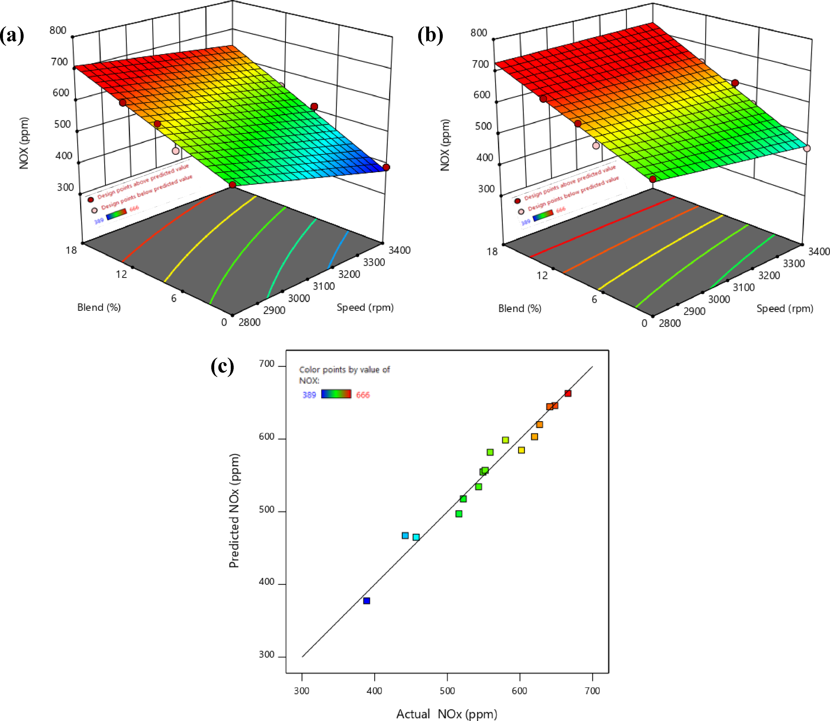
Comparison of NOx emission (a) at lower load, (b) at higher load, and (c) between actual and predicted values.
The comparison between actual and RSM predicted NOx emission is presented in Figure 10(c). The color points from blue to red color represent the minimum NOx emission of 389 ppm and maximum NOx emission of 666 ppm, respectively. Table 12 signifies ANOVA for reduced quadratic model in the case of NOx emission. The probability distribution with F and p-values of 63.15 and less than 0.05, respectively, indicates greater statistical significance of measured NOx emission. Moreover, the quadratic regression model appeared to be a perfect fit with data points in close proximity with regression line. It indicates the minimum possible deviations between predicted and actual data set values.
Analysis of variance (ANOVA) for reduced quadratic model in the case of NOx emission.
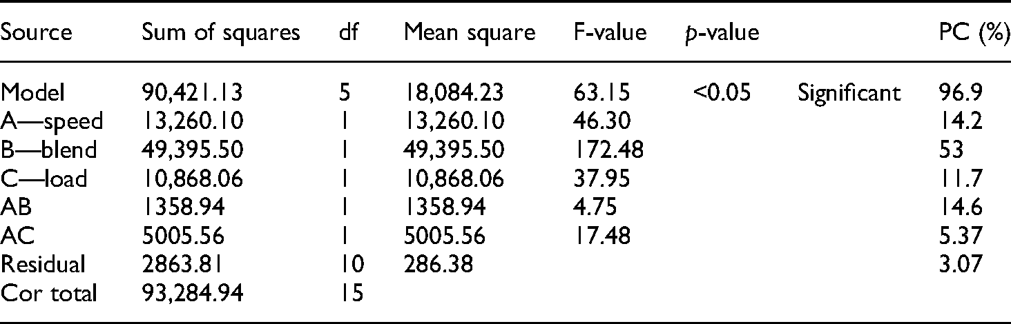
The p-values from Table 12 show that all three factors speed, load, and fuel blends are significant. Moreover, the R2 value of 0.97 was close to positive unity and there was sufficient agreement between predicted and adjusted R2. The predicted R² of 0.94 was in fair compliance with the adjusted R² of 0.95; that is, the difference in between them was equivalent to 0.01. The speed and fuel blend were significantly contributed to aggregated variations with PC% of 14.2% and 53%, respectively, in comparison with load which was 11.7%. For the case of the NOx emission, the p-value given by design expert is less than 0.05, which is testimonial to the fact that we fail to reject null hypothesis and do not have enough evidence to prove the presence of lack of fit in the reduced quadratic model. The best fitted quadratic model from the fit summary was selected due to aliased nature and poor fit of cubic and linear models, respectively. The aliased quadratic model not only allows the estimation of the influence of speed, load, and blend separately on NOx emission, but also allows the interaction between input variables and investigation of their synergic effect on NOx emission. The actual regression equation in the case of NOx emission is shown in equation (8):
Impact on lubricant oil deterioration
The KV, FP, TAN, and ash content are ascertained as deteriorated lubricant oil characteristics for the SI engine and are optimized through RSM technique.
Experimental and predicted KV
The KV is the utmost significant factor that impacts fluid ability of the lubricant oil. The higher friction and wear inside an engine can be credited due to unavailability of sufficient lubricant oil between mating parts. 60 The KV of lubricant oil was calculated using standard ASTM procedure D445. The variation in the trend of the KV of lubricant oil that runs on various methanol–gasoline fuel blends at lower load is shown in Figure 11(a). The decrease of 9.62%, 8.47%, 7.77%, and 6.68% in KV of degraded lubricant oil was observed for M0, M6, M12, and M18 in contrast to fresh lubricant oil at lower load, respectively. It can be credited due to fuel dilution and collapse of lubricant oil molecular structure. 33 However, the KV of degraded lubricant oil for M6, M12, and M18 was 1.15%, 1.85%, and 2.94% higher than that of M0. The KV for methanol blended gasoline fuels declines less because of assimilation of sludges, wear particles, and oxides in the lubricant oil. Figure 11(b) indicates the trend of KV for test fuels range from M0 to M18 with gap of 6% methanol concentration in gasoline blend at higher load. The decrease of 12.24%, 11.01%, 9.34%, and 7.23% KV was observed for M0, M6, M12, and M18 in comparison with fresh lubricant oil at higher load, respectively. However, the KV of degraded lubricant oil for M6, M12, and M18 was 1.23%, 2.90%, and 5.01% higher than that of M0. The higher decrease in KV for gasoline and lower methanol concentrated blended fuels under higher load setting can be reasoned by higher fuel consumption and more fuel dilution in lubricant oil.

Comparison of kinematic viscosity (KV) (a) at lower load, (b) at higher load, and (c) between actual and predicted values.
The comparison between actual and RSM predicted KV of lubricant oil is presented in Figure 11(c). The color points from blue to red color represent the minimum KV of 12.31cst and maximum KV of 13.21cst respectively. Table 13 signifies ANOVA for reduced quadratic model in the case of KV. Moreover, the quadratic regression model appeared to be a perfect fit with data points in close proximity with regression line. It indicates the minimum possible deviations between predicted and actual data set values.
Analysis of variance (ANOVA) for reduced quadratic model in the case of kinematic viscosity (KV).

The probability distribution with F and p-values of 86.09 and smaller than 0.05, respectively, indicates greater statistical significance of measured KV. The p-values from Table 13 show that all three factors including speed, load, and fuel blends are significant. Moreover, the R2 value of 0.98 was close to positive unity and there was sufficient agreement between predicted and adjusted R2. The predicted R² of 0.95 was in fair compliance with the adjusted R² of 0.97; that is, the difference in between them was equivalent to 0.02. The fuel blend and load were significantly contributed to aggregated variations with PC% of 27.5% and 13.7%, respectively, in comparison with speed which was 2.50%. For the case of the KV of lubricant oil, the p-value given by design expert is less than 0.05, which is testimonial to the fact that we fail to reject null hypothesis and do not have enough evidence to prove the presence of lack of fit in the reduced quadratic model. The best fitted quadratic model from the fit summary was selected due to aliased nature and poor fit of cubic and linear models, respectively. The aliased quadratic model not only allows the estimation of the influence of speed, load, and blend separately on KV of lubricant oil, but also allows the interaction between input variables and investigation of their synergic effect on KV of lubricant oil. The actual KV regression equation is show in equation (9):
Experimental and predicted FP
FP is the least temperature beyond which vapors of the lubricant oil quickly ignites in the presence of ignition source. The FP of lubricant oils operated on various test fuels is determined by following ASTM D92 standard. The maximum operating limit of lubricant oil is dependent on FP as it determines the fire safety of oil applications. The lower FP signifies a hazard during operations of lubricant oil which could be responsible for a malfunction in system. The variation in the trend of the FP of lubricant oil for various methanol–gasoline fuel blends at lower load is shown in Figure 12(a). The higher decrease in FP of lubricant oil in the case of M0 is eminent from Figure 12(a). The blending of volatile fuel in lubricant oil mainly responsible for decrease in its flash point.35,61 The decrease of 14%, 11%, 9%, and 7% FP was observed for degraded lubricant oil for M0, M6, M12, and M18, respectively, in comparison with fresh lubricant oil at lower load. However, the FP of degraded lubricant oil for M6, M12, and M18 was 3%, 5%, and 7% higher than that of M0, respectively, at lower load. It can be credited due to more latent heat of evaporation and less volatile nature of methanol. Figure 12(b) indicates the trend of FP for the test fuels range from M0 to M18 with gap of 6% methanol concentration in gasoline blend at higher load. The FP of degraded lubricant oil for M0, M6, M12, and M18 are declined by 18%, 14%, 12%, and 8% in comparison with fresh lubricant oil at higher load, respectively. However, the FP of degraded lubricant oil for M6, M12, and M18 was 4%, 6%, and 10% higher than that of M0, respectively, at higher load. M18 behaves better as fuel in terms of FP when compared with other test fuels due to less volatile nature and more latent heat of vaporization of methanol.
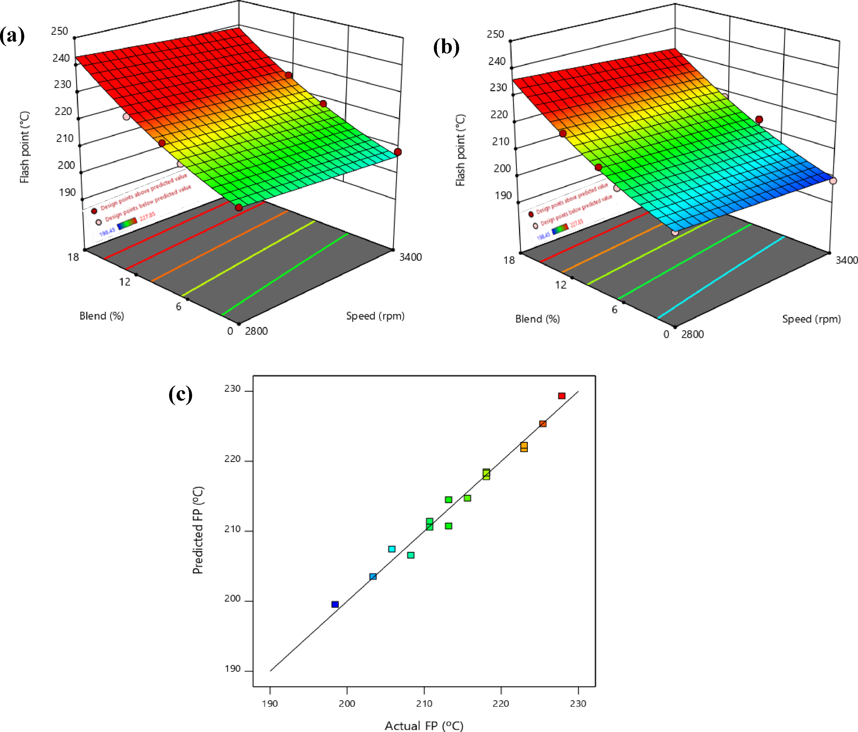
Comparison of flash point (FP) (a) at lower load, (b) at higher load, and (c) between actual and predicted values.
The comparison between actual and RSM predicted FP of lubricant oil is presented in Figure 12(c). The color points from blue to red color represent the minimum FP of 198.45°C and maximum FP of 227.85°C, respectively. Table 14 signifies the ANOVA for reduced quadratic model in the case of FP. Moreover, the quadratic regression model appeared to be a perfect fit with data points in close proximity with regression line. It indicates the minimum possible deviations between predicted and actual data set values.
Analysis of variance (ANOVA) for reduced quadratic model in the case of flash point (FP).

The probability distribution with F and p-values of 135.87 and smaller than 0.05, respectively, indicates greater statistical significance of measured FP. The p-values from Table 14 show that all three factors such as speed, load, and fuel blends are significant. Moreover, the R2 value of 0.98 was close to positive unity and there was sufficient agreement between predicted and adjusted R2. The predicted R² of 0.96 was in fair compliance with the adjusted R² of 0.97; that is, the difference in between them was equivalent to 0.01. The fuel blend and load were significantly contributed to aggregated variations with PC% of 26.6% and 19.7%, respectively, in comparison with speed which was 6.29%. For the case of the FP of lubricant oil, the p-value given by design expert is less than 0.05, which is testimonial to the fact that we fail to reject null hypothesis and do not have enough evidence to prove the presence of lack of fit in the reduced quadratic model. The best fitted quadratic model from the fit summary was selected due to aliased nature and poor fit of cubic and linear models respectively. The actual FP regression equation is shown in equation (10):
Experimental and predicted TAN
TAN specifies the mass of acids exist in lubricant oil and it was determined by following ASTM D974. TAN is directly linked with lubricant oil oxidation and also accountable for varying chemical configuration of lubricant oil. 31 The variation in the trend of the TAN of lubricant oil for various methanol–gasoline fuel blends at lower load is shown in Figure 13(a). The increase of 19.12%, 26.31%, 31.31%, and 39.51% was observed for TAN of degraded lubricant oil for M0, M6, M12, and M18 when compared with fresh lubricant oil at lower load respectively. However, TAN of degraded lubricant oil for M6, M12, and M18 was 7.19%, 12.19%, and 20.39% higher than that of M0, respectively, at lower load. The higher TAN for methanol blended fuel indicates greater wear rate, contaminants, and sludges inside the engine. Figure 13(b) indicates the trend of TAN for test fuels range from M0 to M18 with gap of 6% methanol concentration in gasoline blend at higher load. TAN of degraded lubricant oil for M0, M6, M12, and M18 raised by 21.22%, 29.31%, 37.42%, and 45.24% in comparison with fresh lubricant oil at higher load, respectively. TAN of degraded lubricant oil for M6, M12, and M18 was 8.09%, 16.20%, and 24.02% higher than that of M0, respectively, at higher load.

Comparison of total acid number (TAN) (a) at lower load, (b) at higher load, and (c) between actual and predicted values.
The comparison between actual and RSM predicted TAN of lubricant oil is presented in Figure 13(c). The color points from blue to red color represent the minimum TAN of 2.08 mg/g KOH and maximum TAN of 2.55 mg/g KOH, respectively. Table 15 shows ANOVA for reduced quadratic model in the case of TAN. Moreover, the quadratic regression model appeared to be a perfect fit with data points in close proximity with regression line. It indicates the minimum possible deviations between predicted and actual data set values.
Analysis of variance (ANOVA) for reduced quadratic model in the case of TAN.

The probability distribution with F and

Experimental and predicted ash content
Ash content is key factor to evaluate the pureness of lubricant oil. It indicates the solid residue that persisted in lubricant oil as a result of fuel burning. 62 It also signifies noncombustible constituents that persisted as an ash afterward fuel burning. The constituents are sludges, atmospheric dust, thermally decomposed particles, and wear debris. ASTM D482 standard was opted to determine the ash content of lubricant oil operated on test fuels. The variation in the trend of the ash content of lubricant oil which operated on various methanol–gasoline fuel blends at lower load is shown in Figure 14(a). The increase of 1.96%, 2.49%, 2.94%, and 3.45% was observed for ash content in degraded lubricant oil for M0, M6, M12, and M18 in comparison with fresh lubricant oil at lower load, respectively. However, the ash in degraded lubricant oil for M6, M12, and M18 was 0.53%, 0.98%, and 1.49% higher than that of M0, respectively, at lower load. Figure 14(b) indicates the trend of ash content for the test fuels range from M0 to M18 with interval of 6% methanol concentration in gasoline blend at higher load. The increase of 2.01%, 2.61%, 3.10%, and 3.93% was found for ash content for M0, M6, M12, and M18 when compared with fresh lubricant oil at higher load, respectively. However, the ash content in degraded lubricant oil for M6, M12, and M18 was 0.60%, 1.09%, and 1.92% higher than that of M0, respectively, at higher load. The higher ash content in the case of methanol blended fuel indicates more wear rate, contamination, unburned particles, and sludges inside the lubricant oil for these blended fuels.

Comparison of ash content (a) at lower load, (b) at higher load, and (c) between actual and predicted values.
The comparison between actual and RSM predicted ash content of lubricant oil is presented in Figure 14(c). The color points from blue to red color represent the minimum ash content of 1.96%wt and maximum ash content of 4.34%wt, respectively. Table 16 shows ANOVA for reduced quadratic model in the case of ash content. Moreover, the quadratic regression model appeared to be a perfect fit with data points in close proximity with regression line. It indicates the minimum possible deviations between predicted and actual data set value.
Analysis of variance (ANOVA) for reduced quadratic model in the case of ash content.
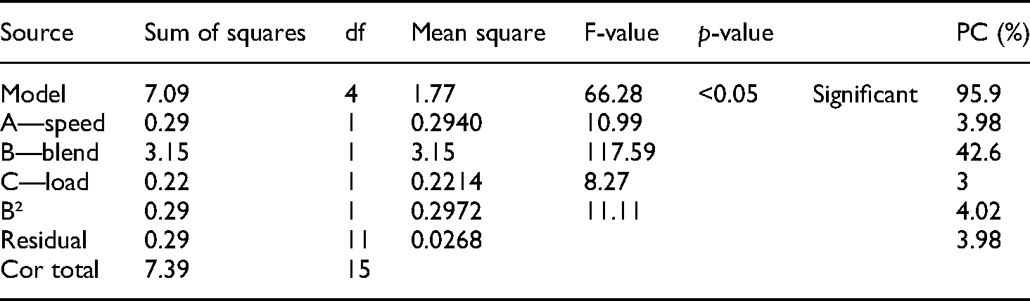
The probability distribution with F and p-values of 66.28 and smaller than 0.05, respectively, indicates greater statistical significance of measured ash content. The p-values from Table 16 show that all three factors speed, load, and fuel blends are significant. Moreover, the R2 value of 0.96 was close to positive unity and there was sufficient agreement between predicted and adjusted R2. The predicted R² of 0.92 was in fair compliance with the adjusted R² of 0.95; that is, the difference in between them was equivalent to 0.03. The speed and fuel blend were significantly contributed to aggregated variations with PC% of 3.98% and 42.6%, respectively, in comparison with load of 3%. For the case of the ash content of lubricant oil, the p-value given by design expert is less than 0.05, which is testimonial to fact that we fail to reject null hypothesis and do not have enough evidence to prove the presence of lack of fit in the reduced quadratic model. The best fitted quadratic model from the fit summary was selected due to aliased nature and poor fit of cubic and linear models, respectively. The actual regression equation for ash content is given by equation (12):
RSM-based optimization
The RSM-based optimization is a robust approach to recognize the optimized conditions by altering the input factors for achieving desirable output(s). It establishes relation between input and response variables and also provides a path for understanding the detailed trends. In the current work, the numerical optimization function of Design Expert software was utilized for optimizing the emission and performance characteristics of an engine along with physicochemical characteristics of lubricant oil. The optimization setup, as shown in Table 17, is aimed at maximizing torque, BP, BTE, and FP while minimizing BSFC, CO, CO2, HC, NOx, KV, TAN, and ash content. All the output variables have been given equal importance and are assigned with the default weight of 3. The optimized operating conditions for engine as recognized by RSM model were 40 psi load, 3400 rpm, and methanol–gasoline blend with 8% methanol in 92% gasoline by volume (M8). The response variables corresponding to these optimized conditions were 2137.13 watt BP, 6.08 N-m torque, 0.37 kg/kwh BSFC, 22.10% BTE, 4.02% CO emission, 7.15% CO2 emission, 134.12 ppm HC emission, 517.02 ppm NOx emission, 12.44 cst KV, 203.77°C FP, 2.23 mg/g KOH TAN, and 2.65%wt ash content. The statistical reliability of optimization for the overall responses was analyzed through composite desirability (D). It is a unitless value ranging from 0 to 1, with value close to 1 representing the most effective optimization. In the present study, composite desirability comes to be 0.73, which is a clear indication that optimization settings have attained favorable outcomes for all responses. Moreover, for deep insight into optimization model and apprehending the impact of individual response variables, individual desirability (d) of each response has been studied and plotted in Figure 15. The maximum and minimum individual desirabilites were observed for torque (0.94) and FP (0.57), respectively. These numerical values show that reducing the torque would impart the greatest variations in the model while maximizing the FP would be responsible for minimum variations. Studied from emissions perspective, it is evident that highest d of 0.6976 was observed for HC emissions while lowest (0.570) for carbon monoxide emissions, with NOx and CO2 having intermediate values. Thus, the d-values for emissions establish the fact that for increasing the reliability of RSM model in terms of collective optimization, the most reliable path would be to contain HC emission as that would important the highest desirable variation.

Desirability chart.
Optimization setup.

TAN: total acid number.
The contour plot for optimization is shown in Figure 16, which shows the variation of D with speed and blend plotted over the entire range. The defined color coding regime shows that at higher speed, higher loading condition, and blend percentages below 9%, the light green color predominantly holds and could be declared as region of higher composite desirability. Onwards from these extremes, the whole region is blue which shows the D values close to 0. Thus, from contour desirability plot, a comprehensive variation of D values could be studied for the whole experimental range.

Contour desirability plot.
Once we are done with the optimization, next it would be necessary to validate the reliability of obtained results. Therefore, an experimentation corresponding to identified optimized conditions would be the most effective way. RSM-based multi-objective optimized results were then validated through experiment. The engine was operated at the optimal values of load, speed, and fuel blend concentration for recording the response variables. The absolute percentage error (APE) among empirical results and RSM predicted results were calculated (Table 18). The predicted results demonstrated a reasonable compliance with empirical results, with APE of all responses under 5%. However, the maximum APE of 4.68% was obtained for FP which might be owing to inefficient desirability as a consequence of manual recording during experimentation. The least APE of 1.57% was obtained for torque because of highest desirability. Overall, the RSM predicted results under developed models are effective and viable.
Comparison between RSM optimized and experimental values.

APE: absolute percentage error; RSM: response surface methodology; TAN: total acid number.
Conclusions
This study has significantly evaluated the impact of distinct test fuels (M0, M6, M12, and M18) on engine's performance and emissions accompanied by their influence on lubricant oil degradation through novel integration of experimental and statistical techniques. The main outcomes of this study are:
BP showed distinctively improved performance with 6.84% and 8.85% higher power for M6 and M12 in comparison with gasoline at low load. BTE showed average increase of 19%, 20%, and 22% for M6, M12, and M18 when compared with base fuel at higher loading conditions. Methanol blending emerged favorable in terms of clean environment with 8.68%, 18.62%, and 28.78% reduced carbon monoxide emissions for M6, M12, and M18 in comparison with M0. Similarly, the greenhouse emissions for M12 and M18 showed average 9.85% and 14% reduction compared to gasoline. The lubricating oil degradation rate was higher for methanol blended fuels when compared with M0 for straight 120 h of engine operation. TAN of degraded lubricant oil for M6, M12, and M18 was 8.09%, 16.20%, and 24.02% higher than that of M0, respectively, at higher load. While the ash content in degraded lubricant oil for M6, M12, and M18 was 0.60%, 1.09%, and 1.92% higher than that of M0, respectively, at higher load. The RSM identified M8, speed of 3400 rpm, and load of 40 psi as optimized conditions for best engine performance, reduced emissions, and minimum lubricating oil deterioration. The operating parameters corresponding to RSM optimized conditions were 2137.13 watt BP, 6.08 N-m torque, 0.37 kg/kwh BSFC, 22.10% BTE, 4.02% CO emission, 7.15% CO2 emission, 134.12 ppm HC emission, 517.02 ppm NOx emission, 12.44 cst KV, 203.77°C FP, 2.23 mg/g KOH TAN, and 2.65%wt ash content. The composite desirability (0.73) was in close proximity of unity which showed reliable and efficient multi-objective optimization. The comparison between predicted and empirical results showed overall APE below 5% which validated the accuracy of RSM prediction.
In context of conclusions drafted from the current study, it could be established that utilization of RSM for engineering applications governs an easy and reliable optimization involving various factors and trends. Moreover, the technique becomes of primal importance and could be effectively used for prediction beyond the designated parameters range and thus could save enormous time and capital. Similarly, the study gives an important insight into lubricating oil deterioration with oxygenated fuel which could be extended in future for developing oils with novel additives that could resist the wear damage and improve the overall life cycle of oil.
Footnotes
Declaration of conflicting interests
The author(s) declared no potential conflicts of interest with respect to the research, authorship, and/or publication of this article.
Funding
The author(s) received no financial support for the research, authorship, and/or publication of this article
Author biographies
Muhammad Ali Ijaz Malik received his BSc in Mechanical Engineering and an MSc Automotive Engineering from UET Lahore in 2017 and 2021, respectively. He is lecturer in Mechanical Engineering Department of Superior University. His research interests are bio-fuels, bio-lubricants, tribology, environmental sustainability and engine performance optimization.
Muhammad Usman received his PhD in Mechanical Engineering from UET Lahore and serving as an assistant professor in the Mechanical Engineering Department of UET Lahore. His research interests are artificial neural networking, biofuels and lubricants.
Maaz Akhtar has extensive experience of research in the field of nano-materials, swelling elastomers and mechanics of materials. He is conducting major research in the institute of Imam Mohammad Ibn Saud Islamic University, Riyadh.
Muhammad Farooq is an associate professor in UET Lahore with major interest in sustainable energies.
Hafiz Muhammad Saleem Iqbal received his PhD in Aerospace Materials from TU Delft and currently conducting research on composites and the optimization of thermal systems.
Muneeb Irshad is working in Department of Physics of UET Lahore with major research interests in synthesis of energy materials.
Muhammad Haris Shah completed his BSc in Mechanical Engineering from University of Engineering and Technology Lahore. His research interest lies in engine performance testing, emission analysis and performance optimization.