Sage Journals: Discover world-class research

Abstract

The deployment of methanol like alternative fuels in engines is a necessity of the present time to comprehend power requirements and environmental pollution. Furthermore, a comprehensive prediction of the impact of the methanol-gasoline blend on engine characteristics is also required in the era of artificial intelligence. The current study analyzes and compares the experimental and Artificial Neural Network (ANN) aided performance and emissions of four-stroke, single-cylinder SI engine using methanol-gasoline blends of 0%, 3%, 6%, 9%, 12%, 15%, and 18%. The experiments were performed at engine speeds of 1300–3700 rpm with constant loads of 20 and 40 psi for seven different fractions of fuels. Further, an ANN model has developed setting fuel blends, speed and load as inputs, and exhaust emissions and performance parameters as the target. The dataset was randomly divided into three groups of training (70%), validation (15%), and testing (15%) using MATLAB. The feedforward algorithm was used with tangent sigmoid transfer active function (tansig) and gradient descent with an adaptive learning method. It was observed that the continuous addition of methanol up to 12% (M12) increased the performance of the engine. However, a reduction in emissions was observed except for NO_x emissions. The regression correlation coefficient (R) and the mean relative error (MRE) were in the range of 0.99100–0.99832 and 1.2%–2.4% respectively, while the values of root mean square error were extremely small. The findings depicted that M12 performed better than other fractions. ANN approach was found suitable for accurately predicting the performance and exhaust emissions of small-scaled SI engines.

Keywords

Methanol small scale SI engine environmental pollutants performance prediction ANN

Introduction

The world’s need for fossil fuels to run vehicles and industries is increasing at a disturbing rate.¹ On the other side, the formation of fossil fuels is not an overnight process as it takes quite a large amount of time after the organic matter is being buried under pressure and heat. Hence, the consumption of fossil fuels is increasing at a much faster rate than the formation of fossil fuels themselves. That is why fossil fuels are depleting rapidly, and it is expected that if the same rate of fossil fuel consumption is continued, then they will be diminished around 2112.^2–4 Moreover, the utilization of fossil fuels in vehicles is also responsible for many environmental problems and is hazardous for human health as well. The discharge gases which result from the burning of fossil fuels are the primary cause of global warming, acid rain, smog production, and emissions like carbon dioxide (CO₂), carbon monoxide (CO), nitrogen oxides (NO_x), oxides of Sulphur (SO_x), particulate matters (PM), and hydrocarbons (HC) which are very harmful not only for the environment but also for all the living creatures on the planet.^5–7 This has led researchers to investigate greener fuels for vehicles.⁸

In these hard times, it has become substantially crucial to find alternatives for helping the decrement in fossil fuel depletion. The main alternatives contain alcohol-based fuels (ethanol, methanol, etc.), vegetable oils, gaseous fuels, ethers, fats, and biodiesel.^9–13 Methanol carries the most important properties and characteristics among all the other alternative fuels due to its extensive production from simple raw materials like coal, natural gas, etc.^6,14 Methanol is mainly considered most efficient in the case of spark ignition engines as it results in higher brake power and reduced emissions.^15–19 The high octane number of the methanol makes it more adaptive towards running at high compression ratios without knocking.^17,20–22

The failure of classical modeling methods and techniques has led researchers to look for alternatives. Artificial Neural Network (ANN) is being used in engineering and scientific applications for its ability to provide solutions for complex non-linear problems. The ability of prediction of ANN makes it a unique statistical tool that estimates and provides the results based on experimental data and conditions. It uses actual data to train and validate the network for the prediction of results.²³ It also provides room for retraining and reassessing the network if the input data is varied.²⁴ The summary of experimental and ANN working is presented in Figure 1.

Figure 1.

Graphical abstract.

Literature survey

Methanol-gasoline blends have demonstrated that with the increase in the ratio of the methanol in the blend, the emissions are reduced by a generous amount such as when M85 is used, the CO and NO_x emissions are reduced by about 25% and 80% effectively.¹⁸ The conversion of emissions can also be optimized with the help of devices such as a three-way catalytic converter (TWC). The M30 is used at 5°C during the cold start and warming up the process, and results reveal a 50% reduction in HC emissions in the cold start. On the other hand, during the warming-up process further 30% and 50% reduction in HC emissions along with CO emissions, respectively, and the increase in the EGT aids in the activation of TWC.¹⁹ The emissions are also dependent on the wheel power, and the speed as the comparison between the ethanol-gasoline and methanol-gasoline blends showed that at the speed of 80 km/h, HC and CO emissions were decreased to a reasonable amount. This trend is not followed at the speed of 100 km/h at 15 kW due to the increment in the air-fuel equivalence ratio.^20,25

In this study, the blend of methanol is tested against the various performance indicators of the engine such as brake power (BP), Torque, brake thermal efficiency (BTE), brake specific fuel consumption (BSFC), and exhaust gas temperature (EGT). Apart from the performance characteristics, the emissions parameters of the engine including CO₂, CO, NO_x, and HC are also observed simultaneously. Furthermore, the blend of methanol aids in solving the critical issue of the depletion of fossil fuels and also in the reduction of emissions that are hazardous for the environment. Their evaluation is also concerned with the efficiency of the blend used.

In the previous decade, due to the high compatibility and accuracy of ANN models, the researchers have employed ANN extensively.^26–30 The ANN models have already been employed in internal combustion engines for the prediction of various parameters.^31–44 Sayin et al.⁴⁵ employed ANN for a gasoline engine study and produced results in a range of 0.983–0.99 for the correlation coefficient. The proposed model of Cay et al.⁴⁶ predicted correlation coefficient (R) values around 0.99 for training and testing data for performance and exhaust of gasoline engines. Kiani et al.⁴⁷ found the correlation coefficient (R) in ranges of 0.71–0.99 for gasoline-ethanol fuel blends. Yusuf and coworkers⁶ suggested accurate ANN models for methanol engine performance. They found the regression coefficient close to 1 for the network structure of 4-7-1 performance indicators with mean errors in less than 5% range. Kapusuz et al.⁴⁸ predicted the performance of an SI engine with ethanol-methanol blends and concluded that a mixture M11E1 (Methanol 11%, Ethanol 1%) produced the best performance and the regression coefficient was in the range 0.931–0.990. Samet et al. used a diesel engine with diethyl ether blend up to 10%. The ANN model predicted results with the regression coefficient (R²) in the range of 0.964–0.9878 and with MRE values in an interval of 0.51%–4.8%.

In light of the literature studied, the significance of the accuracy and compatibility of ANN models in internal combustion engines is undeniable. Researchers have employed ANN for SI engines with alcoholic and hydrogen blends as well as with hydrogen. This article will widen the scope of the use of ANN in SI engines with methanol blends. The effect of fuel ratio along with load and engine speed are comprehensively studied in this article and the accuracy of the predictive model of ANN is evaluated for small-scale single-cylinder engines.

Experimental work

Experimental setup

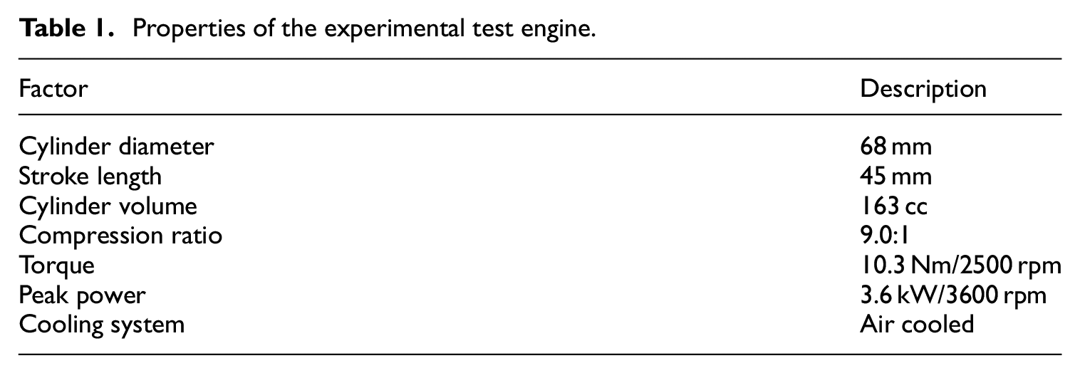
The experimental setup included a four-stroke, single-cylinder, and spark ignition (Honda GX160) engine. The characteristics of the engine are presented in Table 1. Testing was performed without any modification in the engine structure. A 7-inch Dynomite (water-brake) dynamometer was used for testing. A specially designed mild steel shaft was used to connect the engine with the dynamometer. The emissions of the engine were measured using an EMS-5002 emission analyzer. The measuring cylinder of 500 ml with 0.5 ml grading was used to supply the fuel and measure the fuel flow.⁴⁹ A thermocouple based; digital thermometer was used to measure the EGT. There were seven different cylinders used in the experimentation, each for a different methanol-gasoline blend. The load was applied to the dynamometer using the piping system and pump with water as a working fluid. The schematic diagram of the experimental setup is given in Figure 2.

Table 1.

Properties of the experimental test engine.

Factor	Description
Cylinder diameter	68 mm
Stroke length	45 mm
Cylinder volume	163 cc
Compression ratio	9.0:1
Torque	10.3 Nm/2500 rpm
Peak power	3.6 kW/3600 rpm
Cooling system	Air cooled

Figure 2.

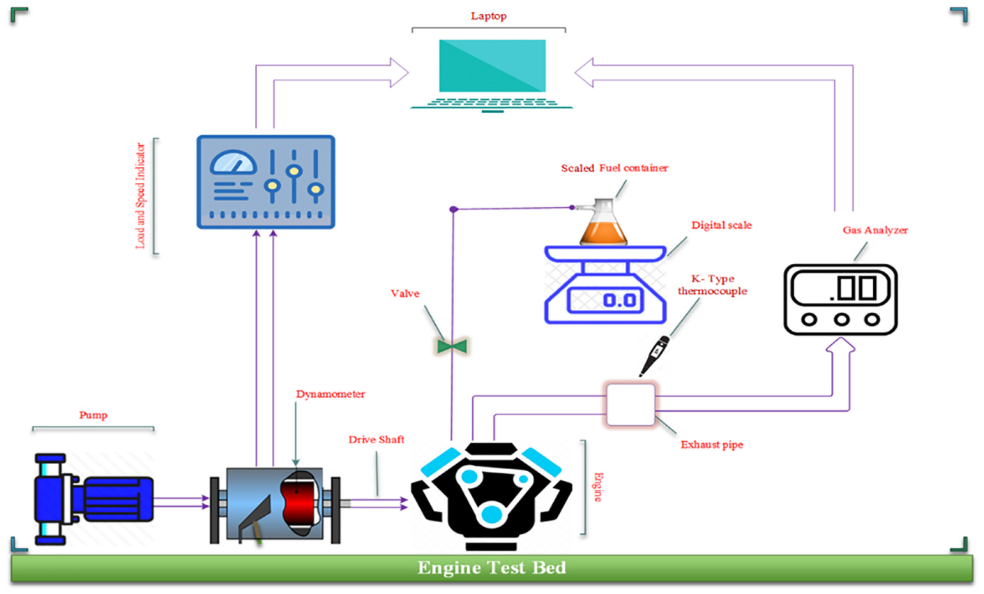
Schematic of engine test bed and experimental setup.

Fuel preparation

The gasoline was obtained from Pakistan State Oil Company and used as a reference for all blends. The properties of gasoline (M0) are presented in Table 2. The methanol was obtained from the merchandise of Merck⁵⁰ and added in gasoline. Methanol was used in concentrations of 3%, 6%, 9%, 12%, 15%, and 18% by volume with gasoline represented as M3, M6, M9, M12, M15, and M18 respectively. To prepare a completely homogenous mixture of the fuels, the mixture was stirred continuously using a magnetic stirrer (hot plate 78-1) for 20 min. The fuel preparation schematic is demonstrated in Figure 3. The fuel blends were poured into the cylinder within 2 min of their preparation to ensure homogeneity. The properties of pure methanol (M100) and the fuel blends are also shown in Table 2.

Table 2.

Properties of methanol blended fuels.

Properties	Fuel blends
	M0	M3	M6	M9	M12	M15	M18	M100
Density (kg/m³)	731	732.83	734.66	736.49	738.32	740.15	741.98	792
Viscosity (mPa.s)	0.602	0.60176	0.60152	0.60128	0.60104	0.6008	0.60056	.594
Octane number	92	92.9	93.8	94.7	95.6	96.5	97.4	122
Calorific value (kJ/kg)	44200	43567	42934	42301	41668	41035	40402	23100
Oxygen content % v/v	0	1.5	3	4.5	6	7.5	9	50

Figure 3.

Fuel preparation.

Testing procedure

The testing was carried out by increasing the engine speed from 1300 rpm to 3700 rpm in equal increments of 300 rpm to 3700 rpm using the throttle. There were two variations of engine loads applied at every speed. Initially, the engine was started using only gasoline until it reached a steady-state operation. To ensure the homogeneity of the mixture and to avoid moisture, the blends were prepared only 10 min before the experimentation.

The test was performed three times under each condition to ensure the accuracy and average of three readings were taken. The value of engine speed and the applied load was noted using the Dynomite 2010 software, fuel consumption was measured while the torque, BSFC, brake power, and BTE was computed using heating values and density. The EGT was measured using a thermometer and CO₂, CO, HC, and NO_x emissions were measured from the EMS emission analyzer.

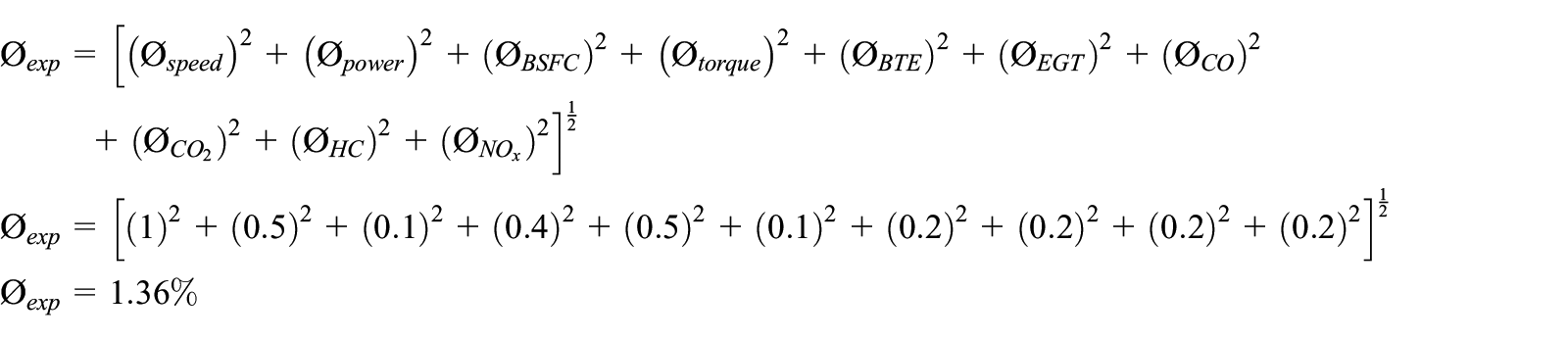
Uncertainty analysis

The degree of accuracy of measured experimental parameters and is determined using uncertainty analysis. The physical limitation of the experimental setup provides the magnitude of the error in each measurement. These error percentages for performance and emissions parameters are given in Table 3. The overall experimental uncertainty was calculated using known errors in the parameters with the help of the general equation (1)⁴⁹

\frac{\emptyset_{y}}{y} = \sqrt{\sum_{i = 1}^{n} {(\frac{1}{y} \frac{\partial y}{\partial x_{i}} \emptyset_{x_{i}})}^{2}}

(1)

Table 3.

Uncertainties and measurement accuracies of parameters.

Parameter	Measurement range	Accuracy	Uncertainty (%)
Torque	$0 - 45 N m$	$\pm 0.1 N m$	$\pm 1$
Speed	$0 - 8000 rpm$	$\pm 5 rpm$	$\pm 0.5$
Power	$0 - 50 kW$	$\pm 0.05 kW$	$\pm 0.1$
SFC	-	$\pm 0.1 g / kWh$	$\pm 0.4$
BTE	-	-	$\pm 0.5$
EGT	$0 - 1300 ° C$	$\pm 1 ° C$	$\pm 0.1$
CO	$0 - 18 vol %$	$\pm 0.01 vol %$	$\pm 0.2$
$C O_{2}$	$0 - 18 vol %$	$\pm 0.01 vol %$	$\pm 0.2$
HC	$0 - 5000 ppm$	$\pm 1 ppm$	$\pm 0.2$
$N O_{X}$	$0 - 5000 ppm$	$\pm 1 ppm$	$\pm 0.2$

Where, $x_{i}$ are the known physical parameters; $\emptyset_{y}$ and $\emptyset_{x_{i}}$ are errors or uncertainties in $y$ and $x_{i}$ respectively. Putting the error percentages from Table 3 in equation (1), the uncertainty of the experiment was calculated as follow;⁵¹

\begin{matrix} \emptyset_{\exp} = [{(\emptyset_{speed})}^{2} + {(\emptyset_{power})}^{2} + {(\emptyset_{BSFC})}^{2} + {(\emptyset_{torque})}^{2} + {(\emptyset_{BTE})}^{2} + {(\emptyset_{EGT})}^{2} + {(\emptyset_{CO})}^{2} \\ {+ {(\emptyset_{C O_{2}})}^{2} + {(\emptyset_{HC})}^{2} + {(\emptyset_{N O_{x}})}^{2}]}^{\frac{1}{2}} \\ \emptyset_{\exp} = {[{(1)}^{2} + {(0.5)}^{2} + {(0.1)}^{2} + {(0.4)}^{2} + {(0.5)}^{2} + {(0.1)}^{2} + {(0.2)}^{2} + {(0.2)}^{2} + {(0.2)}^{2} + {(0.2)}^{2}]}^{\frac{1}{2}} \\ \emptyset_{\exp} = 1.36 % \end{matrix}

Experimental results and discussion

Alcoholic fuels generally provide cleaner and smoother combustion in gasoline engines as compared to conventional fuels. The experimental outcomes have demonstrated that methanol increases the torque, brake power, BTE, EGT, and NO_x emissions, whereas, it decreases the BSFC, and emissions indicators like CO, CO₂, and HC.

Performance parameter

The lower heating value of methanol as compared to gasoline with higher energy conversion provides increased output power in smaller engines, reduces the BSFC, and increases the BTE. The brake power increases due to methanol because of its oxygen content, which makes the mixture lean, hence improves the combustion of fuel.^18,51 BTE is a measure of the useful work done by the combustion of fuels.^52,53 The BSFC decreases with the increase of brake power while BTE increases.

Brake power

The change in the BP of the engine against engine speeds for various blends is given in Figure 4(a). The increase in methanol content increased the BP of the engine for each testing speed. Since the BP is directly proportional to the engine speed hence it demonstrated consistent increases with the increase in engine speed. The hydraulic load increment from 20 to 40 psi also favored the increase in BP due to increments in the torque.⁵⁴ The percentage increase at the load of 20 psi is 2.71%, 11.76%, 17.51%, 19.76%, 11.83%, and −0.27% and at the load of 40 psi is 5.62%, 6.83%, 7.28%, 10.02%, 6.73%, and 2.73% for blends of M3, M6, M9, M12, M15, and M18 respectively. Since the evaporation heat of gasoline is lesser than methanol, the density of charge increases and higher power was produced.⁵⁵ The increased oxygen content of methanol improves energy conversion due to smoother combustion, which tends to increase the brake power. The brake power showed a significant decrease with the increase of methanol beyond 12% because the increasing content of methanol in blends significantly reduces the calorific value of the blend.⁵⁶ The BP of M18 was reduced marginally and was lesser than gasoline at higher engine speeds. The increase in the concentration of methanol in the fuel increased the power at all speeds to a certain amount.⁵⁷ Figure 4(b) demonstrates averages of brake power for each fuel blend over a complete range of speed. The varying speed generated average value for M0, M3, M6, M9, M12, M15, and M18 fuel blends as 904.0, 928.5, 1010.3, 1062.2, 1082.6, 1010.9, and 901.6W at 20 psi load and 1288.3, 1360.7, 1376.2, 1382.1, 1417.4, 1375.0, and1323.4 W at 40 psi load respectively. The highest increase in brake power was recorded for M12 as 19.76% for 20 psi load and 10.02% for 40 psi load.

Figure 4.

(a) Variation of brake power against engine speed, and (b) average values of brake power for various blends.

Torque

The variation in the torque of the engine against engine speed for different blends is given in Figure 5(a). The continuous increase of methanol in gasoline increased the torque for the entire speed range. The increase of speed also favored the increase of torque as at higher speeds due to faster burning of fuel the energy input and output increase.⁵⁴ The increase in load increased the torque significantly due to an increase in applied force. The percentage increase at the load of 20 psi is 2.71%, 11.76%, 17.51%, 19.76%, 11.83%, and −0.27% and at the load of 40 psi is 5.62%, 6.83%, 7.28%, 10.02%, 6.73%, and 2.73% for blends of M3, M6, M9, M12, M15, and M18 respectively. The addition of methanol produces lean mixtures and results in efficient burning.⁵⁶ The knocking decreases due to an increase in octane number with the addition of methanol so timing is advanced, producing higher cylinder pressure and in return higher torque.⁵⁵ The decrease in torque by the addition of methanol higher than 12% is due to a significant decrease in input power. The calorific value of methanol is almost half of gasoline and so the continuous addition decreased the energy input and caused the output torque to drop. Figure 5(b) demonstrates the average values of torque over the entire speed range at different loads for all fuel blends. The varying speed generated average value of torque for M0, M3, M6, M9, M12, M15, and M18 fuel blends as 3.20, 3.29, 3.58, 3.75, 3.83, 3.57, and 3.19 Nm at 20 psi load and 4.62, 4.91, 4.98, 5.01, 5.14, 4.98, and 4.76 Nm at 40 psi load respectively. The highest increase in torque was recorded for M12 as 19.62% for 20 psi load and 12.19% for 40 psi load.

Figure 5.

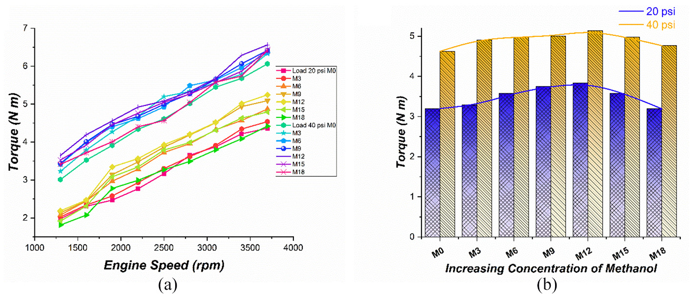
(a) Variation of experimental torque against engine speed, and (b) average values of torque for various blends.

Brake thermal efficiency

The effect of methanol blends on BTE is presented in Figure 6(a). The BTE increases uniformly for 1300–2800 rpm and then it decreases at a load of 20 psi however, it increases uniformly for 1300–3100 rpm and then shows a sudden increase for 3400 rpm for 40 psi load and decreases afterward. The increase of BTE at lower speeds is due to the creation of a lean mixture. At higher speeds, the combustion is fast and abrupt, so BTE decreases rapidly.⁵⁶ The maximum BTE for all fuels was obtained at 2800 rpm for 20 psi load and 3400 rpm for 40 psi load due to the highest energy conversion. The higher power output for a load of 40 psi generates higher BTE. The percentage increase at the load of 20 psi is 2.66%, 6.28%, 9.53%, 11.30%, 4.88%, and −0.63% at the load of 40 psi is 5.61%, 9.23%, 13.26%, 15.41%, 11.45%, and 6.40% for blends of M3, M6, M9, M12, M15, and M18 respectively. The increment of power, smoother and efficient burning were the major factors in increasing the BTE.^52,53 The efficiency increase is also due to isochoric combustion and less flow and dissociation losses due to a higher density of methanol.⁵⁸ Figure 6(b) demonstrates the average values of BTE over the complete speed range at different loads for each fuel blend. The varying speed at constant load generated average value of thermal efficiency for M0, M3, M6, M9, M12, M15, and M18 fuel blends as 14.66%, 15.05%, 15.56%, 16.01%, 16.31%, 15.37%, and 14.57% at 20 psi load and 17.36%, 18.33% 18.96%, 19.66%, 20.03%, 19.35%, and 18.47% at 40 psi load respectively. The highest increase in thermal efficiency was recorded for M12 as 11.30% for 20 psi load and 15.41% for 40 psi load.

Figure 6.

(a) Variation of experimental BTE against engine speed, and (b) average values of BTE for various blends.

Brake specific fuel consumption

The variation in the BSFC of the engine against engine speed for various blends is given in Figure 7(a). The decrease of BSFC at lower speeds because of a significant increase in BP. At higher speeds, the combustion is fast and abrupt, so BSFC increases rapidly.⁵⁶ The minimum BSFC for all fuels was obtained at 2800 rpm for 20 psi load and 3400 rpm for 40 psi load. The higher power output for the load of 40 psi generated a smaller BSFC. The percentage decrease at the load of 20 psi is 0.61%, 1.36%, 2.57%, 2.93%, and −4.49% at the load of 40 psi is 2.36%, 4.16%, 6.08%, 6.40%, and 1.58% for blends of M3, M6, M9, M12, and M15 respectively. The fuel blend of M18 showed an increase in BSFC by 11.82% for 20 psi and 5.03% for 40 psi load. The BSFC decreased for smaller methanol blends due to higher heat of vaporization and smaller AFR, however, it increased for higher methanol blends.⁵⁹ The BSFC decreased because of the increased fuel density and BMEP of an engine which also results in increasing BTE.^60,61 Figure 7(b) demonstrates the average values of BSFC for the complete speed range at different loads for each fuel blend. The varying speed at constant load generated average value of BSFC for M0, M3, M6, M9, M12, M15, and M18 fuel blends as 0.540, 0.539, 0.532, 0.526, 0.524, 0.564, and 0.603 kg/kWh at 20 psi load and 0.458, 0.447, 0.438, 0.430, 0.428, 0.450 and 0.481 kg/kWh at 40 psi load respectively. The maximum decrement in BSFC was noted for M12 as 2.93% for 20 psi load and 6.40% for 40 psi load and the maximum increase was obtained for M18 as 11.82% for 20 psi and 5.03% for 40 psi load.

Figure 7.

(a) Variation of experimental BSFC against engine speed, and (b) average values of BSFC for various blends.

Exhaust Gas Temperature

The efficient burning of the fuel due to increased methanol content increases the in-cylinder temperature. The EGT indicates the heat generated during the combustion of blends.⁶² So, the increase in EGT due to an increase in methanol content as demonstrated in Figure 8(a) because of an increase in oxygen percentage in the fuel. The percentage increase in the EGT is 3.38%, 11.43%, 19.48%, 24.65%, 25.53%, and 27.38% at the load of 20 psi and 4.27%, 7.06%, 10.70%, 13.26%, 16.98% and 18.95% at 40 psi for blends of M3, M6, M9, M12, M15, and M18 respectively.

Figure 8.

(a) Variation of experimental EGT against engine speed, and (b) average values of EGT for various blends.

Figure 8(b) demonstrates the average values of EGT over the complete speed range at both loads for each fuel blend. The varying speed at constant load generated average value of EGT for M0, M3, M6, M9, M12, M15, and M18 fuel blends as 243, 251, 271, 290, 303, 305, and 309°C at 20 psi load and 299, 312, 320, 331, 339, 350, and $356 ° C$ at 40 psi load respectively. The highest increase in EGT was recorded for M18 as 27.38% at 20 psi load and 18.95% at 40 psi load.

Emission Parameters

The lean mixture produced due to increased overall oxygen content of fuel with the addition of methanol helped in efficient burning. This helps to produce a higher amount of oxygen that resulted in cleaner combustion and reduction of carbon oxides and HC. However, the increase in EGT produces a higher amount of NO_x as nitrogen reacts rapidly with oxygen at a higher temperature.

CO Emissions

The evident decrease in the concentrations of CO can be seen with an increase in the concentration of methanol in Figure 9(a). It explains that the combustion is turning towards completion. The AFR reaches towards stoichiometric value as the amount of methanol increases because of the low carbon contents of methanol. The percentage decrease in the CO emissions is 4.66%, 10.19%, 15.17%, 19.36%, 23.87%, and 29.05% at the load of 20 psi and 8.05%, 17.63%, 20.06%, 21.66%, 25.15%, and 27.81% at 40 psi for blends of M3, M6, M9, M12, and M15 respectively. The presence of oxygen also helps to generate a high oxygen-to-fuel ratio which significantly increases the regions of rich fuel inside the combustion chamber.^19,55,56,63

Figure 9.

(a) Variation of experimental CO against engine speed, and (b) average values of CO for various blends.

Figure 9(b) demonstrates the average values of CO emissions over the entire speed range at both loads for each fuel blend. The varying speed at constant load generated average value of CO emissions for M0, M3, M6, M9, M12, M15, and M18 fuel blends as 3.82, 3.64, 3.43, 3.24 3.08, 2.91, and 2.71% by volume at 20 psi load and 2.92, 2.69, 2.41, 2.34, 2.29, 2.19, and 2.11% by volume at 40 psi load respectively. The highest decrease in CO emissions was recorded for M18 as 29.05% for 20 psi load and 27.81% for 40 psi load.

CO₂ Emissions

The significant decrement in the concentrations of CO₂ can be observed with an increase in the methanol content as demonstrated in Figure 10(a). The higher concentrations of methanol decrease the carbon content and increase the oxygen content. The increase in load also decreases the emissions as BSFC was small for higher load and fuel consumption was lower.⁵⁸ The percentage decrease in the CO₂ emissions is 2.23%, 5.05%, 6.65%, 11.18%, 14.07%, and 16.84% at the load of 20 psi and 4.58%, 9.08%, 11.02%, 12.57%, 14.89%, and 16.25% at 40 psi for blends of M3, M6, M9, M12, and M15 respectively. The higher amount of oxygen and low carbon content of methanol decreases CO₂ emissions because of the decrease in carbon to oxygen ratio.⁵⁹

Figure 10.

(a) Variation of experimental CO₂ against engine speed, and (b) average values of CO₂ for various blends.

Figure 10(b) demonstrates the average values of CO₂ emissions over the entire speed range at both loads for each fuel blend. The varying speed at constant load generated average value of CO₂ emissions for M0, M3, M6, M9, M12, M15, and M18 fuel blends as 5.81, 5.66, 5.48, 5.28, 5.05, 4.87, and 4.68% by volume at 20 psi load and 6.03, 5.90, 5.73, 5.63, 5.36, 5.18, and 5.02% by volume at 40 psi load respectively. The highest decrease in CO₂ emissions was recorded for M18 as 16.84% for 20 psi load and 16.25% for 40 psi load.

HC emissions

The decrease in the concentrations of HC with the increase in the concentration of methanol is presented in Figure 11(a). The relative increase in AFR because of the increased percentage of oxygen content in fuel decreases the HC emissions.⁶¹ The percentage decrease in the HC emissions is 2.12%, 4.97%, 7.92%, 11.05%, 14.14%, and 17.04% at the load of 20 psi and 3.51%, 7.53%, 10.81%, 14.66% 18.56%, and 21.68% at 40 psi for blends of M3, M6, M9, M12, and M15 respectively. The emissions are reduced to an efficient and higher combustion rate with an increase in speed.⁶⁴

Figure 11.

(a) Variation of experimental HC against engine speed, and (b) average values of HC for various blends.

Figure 11(b) demonstrates the average values of HC emissions over the complete speed range at both loads for each fuel blend. The varying speed at constant load generated average value of HC emissions for M0, M3, M6, M9, M12, M15, and M18 fuel blends as 230, 225, 219, 212, 205, 198, and 191 ppm at 20 psi load and 199, 192, 184, 178, 170, 162, and 156 ppm at 40 psi load respectively. The highest decrease in HC emissions was recorded for M18 as 17.04% for 20 psi load and 21.68% for 40 psi load.

NO_x emissions

The variation of concentrations of NO_x with the blends of methanol is given in Figure 12(a). There is a substantial increase in NO_x emissions since emissions of NO_x are dependent on the exhaust temperature which increases with load and speed.⁶⁴ Initially, with the increase in exhaust gas temperature, there is an increase in NOx emission contents. It is patently clear from Figure 8(a) and 12(a) that with the increase in the methanol content in the fuel, the NOx emission increases which is quite in line with the increasing trend of exhaust gas temperature. The percentage decrease in the NO_x emissions is 5.49%, 12.54%, 19.19%, 28.73%, 35.81%, and 41.13% at the load of 20 psi and 10.22%, 18.60%, 28.04%, 34.58%, 39.41%, and 45.11% at 40 psi for blends of M3, M6, M9, M12, and M15 respectively. The higher rate of combustion of fuel increases the flame temperature due to which the NO_x emissions increase.⁶¹ Figure 12(b) demonstrates the average values of NO_x emissions over the complete speed range at both loads for each fuel blend. The varying speed at constant load generated average value of NO_x emissions for M0, M3, M6, M9, M12, M15, and M18 fuel blends as 316, 333, 355, 376, 406, 429, and 445 ppm at 20 psi load and 357, 393, 423, 457, 480, 497, and 518 ppm at 40 psi load respectively. The highest decrease in NO_x emissions was recorded for M18 as 41.13% for 20 psi load and 45.11% for 40 psi load.

Figure 12.

(a) Variation of experimental NO_x against engine speed, and (b) average values of NO_x for various blends.

ANN model

Artificial Neural Network (ANN) is a designed statistical model based on the visual processing system of the human brain. It stimulates the performance of the system analytically. This is a widely used powerful technique for processing, analyzing, and predicting the results of non-linear data. There are three layers, consisting of processing particles called neurons; input layer, hidden layer, and output layer. The interlinked structure of weighted biases exists between the neurons of consecutive layers, which transfers the signals.⁶⁵ The model is based on the experimental results. These results are used for training and validation of the ANN model to generate the predicted output under different circumstances. The activation function acts as a function between layers and generates the predicted output using the training data set. The learning process utilizes the concept of RMSE for accuracy (equation (1)). The input layer of the model consists of user-defined entries and generated through experimentation. The prediction of the variables from ANN is generated after the processing of neurons via a specific activation function after training. The iterations in training are performed to reduce the error and once it reaches the required tolerance, training is complete.⁴⁷

RMSE = \sqrt{\frac{1}{n} \sum_{i = 1}^{n} {(t_{i} - p_{i})}^{2}}

(2)

In equation (2), ‘ $t$ ’ is the real output, ‘ $p$ ’ is the predicted output, and ‘ $n$ ’ is the number of entries of the experimental data set.

The proposed network structure for ANN is presented in Figure 13. In total, ten three-layer experimental models of ANN were employed. The first model included the three input nodes: engine speed, load, and blend ratios, a single hidden layer with thirty-two nodes, and an output layer with nine nodes. All the remaining nine models had single output neurons, one for each output. The data was divided into three portions randomly by MATLAB NN Toolbox; training, validation, and testing data set which included 70%, 15%, and 15% respectively. The feedforward network algorithm was used in the hidden and output layer with a hyperbolic tangent sigmoid (tansig) as the active function. The feedforward network provides swift responses on the basis of error ratios generated in each iterations and uses these errors to modify the network to get accurate results in time efficient manner. On the other hand, tansig is improved form of tanh function and have steeper differential as compared to normal sigmoid functions. Owing to these, tansig is highly effective in larger datasets (such as this) due to quick learning and grading. The learning algorithm of gradient descent with adaptive learning (traingda) was selected in the ANN structure. The best results were chosen based on the minimum MRE of experimental and predicted output, defined in equation (2). The correlation coefficient (R) closest to +1 was achieved for the better-predicted outcome. This explains the linear relationship between the experimental and predicted outcome as positive and results are highly accurate.⁶⁶

MRE (%) = \frac{1}{n} \sum_{i = 1}^{n} (| \frac{t_{i} - p_{i}}{t_{i}} | * 100)

(3)

Figure 13.

ANN model structure for SI engine with methanol blended fuels.

The forward feed processes the information using neurons in the first stage and an error is generated. The error is then examined by network comparing the predicted output generated through the ANN with the experimental output. This error is later sent to the input layer in the feedback stage of the network. The communication links are updated, and weighted output is generated by adaptation and retraining. The network performs multiple iterations this way.⁶⁶ The ANN results were generated using the structure demonstrated in Figure 12. The statistical estimation of results was guided by two basic indicators: correlation coefficient (R) and MRE. The statistical estimation in ranges of R > 0.99 and MRE < 3% was set as a defining parameter for the success of the ANN model. If the required values were not achieved in the first loop of 1000 iterations for any statistical indicator, the adaptation rate was varied. The learning rate was set between the step increment of 1.1 and step decrement of 0.9.

ANN results

The prediction of results using the ANN model proved to be highly successful. The first model with the total experimental results of all the parameters generated highly accurate results for each parameter. The comparison of the experimental results and estimated output gave the correlation coefficient (R) of 0.99832 and MRE of 1.95%. The model generated results are presented in Figure 14. After the first success, the ANN model for individual outputs was employed to predict the values comprehensively. The forward feedback algorithm and network structure provided sufficiently accurate results.

Figure 14.

The correlation coefficient values of training, validation and testing data for overall experimental results.

The comparative results for experimental and predicted values of BP, torque, BSFC, BTE, and EGT are presented in Figure 15(a)–(e) respectively. The correlation coefficient for predicted results of torque, BP, BSFC, BTE, and EGT were 0.9972, 0.9982, 0.9910, 0.9932, and 0.9951 respectively. The calculated MREs were 1.8%, 1.4%, 1.3%, 1.5%, and 1.7% for BP, torque, BSFC, BTE, and EGT respectively. The RMSEs were 26.8 W, 0.072 Nm, 0.008 kg/kWh, 0.365%, and 6.686°C for BP, torque, BSFC, BTE, and EGT respectively.

Figure 15.

Predicted results of ANN for the (a) BP, (b) torque, (c) BSFC, (d) BTE, and (e) EGT against experimental results.

The ANN generated estimated values for the performance of small-scale SI engines with methanol blended fuel yielded highly accurate results. It was noted that the designed ANN model predicted the performance of the engine with MRE in the range of 1.3%–1.8% and R values were in the range of 0.99100–0.99825. The RMSE values were also found extremely low in the case. It indicates that the performance of SI engines can be accurately simulated with proper modeling of ANN. Figure 16(a)–(e) represent the comparison of experimental results and ANN predicted outputs against each test case of the original testing scheme for BP, torque, BSFC, BTE, and EGT respectively.

Figure 16.

Comparative analysis of ANN prediction and experimental results for the (a) Brake Power, (b) Torque, (c) BSFC, (d) BTE, and (e) EGT for each test case.

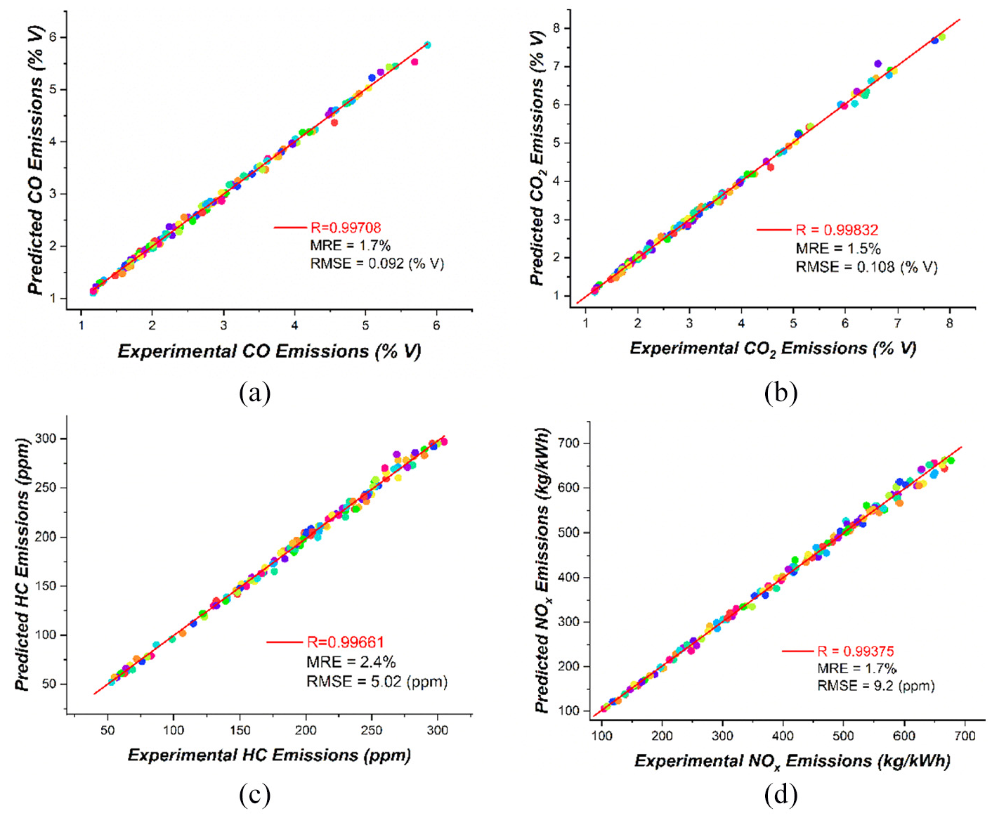
The comparative analysis of experimental and predicted results for CO emissions is presented in Figure 17(a). The results generated via ANN for CO produced the MRE of 1.7%, the R of 0.9971, and the RMSE of 0.092%v. Figure 17(b) indicates the experimental and predicted comparison for $C O_{2}$ emissions. The comparison generated the MRE of 1.5%, the R of 0.9983, and the RMSE of 0.108%v. The comparative analysis for predicted and experimental results of HC emissions is depicted in Figure 17(c). The MRE value, R, and RSME for HC were observed as 2.4%, 0.9966, and 5.02 ppm respectively. Similarly, the comparative results of NO_x emissions are shown in Figure 17(d). The results showed the MRE, R, and RMSE of 1.7%, 0.9937, and 9.2 ppm respectively.

Figure 17.

Predicted results of ANN for the (a) CO, (b) CO₂, (c) HC, and (d) NO_x for each test case.

The ANN-based predicted values for the emissions of a small-scale SI engine with methanol blended fuel produced extremely good results. The ANN model predicted the emissions of the engine with MRE in the range of 1.5%–2.4% and R in the range of 0.99375–0.99832. This shows that the emissions of SI engines can be precisely predicted using an accurate ANN model. Figure 18(a)–(e) represent the comparison of experimental results and ANN predicted outputs against 126 test cases of the original testing scheme for CO, CO₂, HC, and NO_x, respectively. The predicted results were completely inline and demonstrated similar behavior as the experimental outcomes.

Figure 18.

Comparative analysis of ANN prediction and experimental results for the (a) CO, (b) CO₂, (c) HC, and (d) NO_x for each test case.

Conclusions

The use of methanol-gasoline blend (M12) in the small-scale SI engine provided maximum energy conversion into useful work and resulted in increasing torque, BP, and BTE (14.9%, 15.4%, and 13.4% respectively). The BSFC was decreased by 4.7% as compared to M0. The emissions of CO₂, CO, and HC were decreased with the increase of methanol percentage in the fuel blends due to the presence of oxygen content and smaller carbon to hydrogen ratio. The CO, CO₂, and HC were decreased by 28.4%, 16.5%, and 19.4% respectively for M18 in comparison with M0. The higher oxygen and hydrogen content improve the burning thus generating higher heat and associated EGT and NO_x emissions. Therefore, 23.2% and 43.1% increase in EGT and NO_x emissions were observed.

The continuous addition of methanol does not guarantee an increase in BP and BTE. Moreover, BP, torque, and BTE increased up till M12 and then started to decrease. For M18, the increment in BP, torque, and BTE was reduced to 1.4%, 1.2%, and 2.9% as compared to the increments of M12 (15.4%, 14.9%, and 13.4%) respectively. The BSFC also started to increase with the addition of methanol after M12. However, the emission parameters had shown constant behavior with an increase in the concentration of methanol in the fuel.

It is abundantly clear that the ANN generated results were well within the range of the actual experimental results. The acquired results of the ANN verified extremely good statistical correlations. The overall MRE was in the range of 1.3%–2.4%, whereas the R was in the range of 0.99100–0.99832. The RMSE for each parameter was extremely small. The lower error values for each parameter depicted that the ANN could be employed to predict the performance and emissions of a small-scale single-cylinder SI engine accurately. The effect of oxidative fuels on change in engine oil properties is recommended for the future work. The use of methanol in the gasoline engine may significantly alter the characteristics of the engine oil due to its different physico-chemical properties as compared to gasoline fuel. It can be said that ANN can be used to predict the outcomes of any complex and multivariate system providing help in reducing time, cost, and human effort.

Footnotes

Appendix

Declaration of conflicting interests

The author(s) declared no potential conflicts of interest with respect to the research, authorship, and/or publication of this article.

Funding

The author(s) received no financial support for the research, authorship, and/or publication of this article.

ORCID iDs

Ehtasham Ahmed

Muhammad Usman

Author biographies

Ehtasham Ahmed graduated in Mechanical Engineering from University of Engineering and Technology, Lahore in 2020. His research interests includes Internal Combustion Engines, Renewable Energy, Renewable fuels, and AI. He is currently working as Trainee Engineer in Pak Elektron Limited (PEL).

Muhammad Usman is an Assistant Professor at Mechanical Engineering Department, University of Engineering and Technology Lahore-Pakistan. His research interest includes Internal Combustion Engine, Energy, Tribology, AI and Environment.

Sibghatallah Anwar graduated in Mechanical Engineering from UET, Lahore in 2020. During studies, her research interest included Energy, IC Engines and Environment. She is currently working as a trainee engineer at Descon Oxychem Ltd.

Hafiz Muhammad Ahmad is lecturer at Mechanical Engineering Department, University of Engineering and Technology Lahore-Pakistan. His research interest includes Water, Energy, AI and Environment. Currently, he is a PhD scholar

Muhammad Waqar Nasir joined the Department of Mechanical Engineering, UET Lahore as a Lecturer in 2014. He has completed his BSc and MSc degrees in Mechanical Engineering from UET Lahore. Currently, he is a doctoral student. His research interests are mainly focusing on modelling and simulation, characterization and AI.

Muhammad Ali Ijaz Malik joined the Department of Mechanical Engineering, UET Lahore as a student in 2013. Moreover, he has completed Masters in Automotive Engineering from UET Lahore as well. His research interest includes Internal Combustion Engine, Energy, Tribology and Eco-friendly systems.

References

Asif

Muneer

Energy supply, its demand and security issues for developed and emerging economies. Renew Sustain Energy Rev 2007; 11: 1388–1413.

Shafiee

Topal

When will fossil fuel reserves be diminished?

Energ Policy 2009; 37: 181–189.

Höök

Tang

Depletion of fossil fuels and anthropogenic climate change—A review. Energ Policy 2013; 52: 797–809.

Abas

Kalair

Khan

Review of fossil fuels and future energy technologies. Futures 2015; 69: 31–49.

Barbir

Veziroğlu

Plass

HJ.

Environmental damage due to fossil fuels use. Int J Hydrogen Energ 1990; 15: 739–749.

Çay

Korkmaz

Çiçek

, et al. Prediction of engine performance and exhaust emissions for gasoline and methanol using artificial neural network. Energy 2013; 50: 177–186.

Usman

Hayat

Use of CNG and Hi-octane gasoline in SI engine: a comparative study of performance, emission, and lubrication oil deterioration. Energ Sourc Part A: Recover Util Environ Effect 2019: 1–15.

Usman

Hayat

Lubrication, emissions, and performance analyses of LPG and petrol in a motorbike engine: a comparative study. J Chin Inst Eng 2020; 43: 47–57.

Sangeeta Moka

Pande

, et al. Alternative fuels: An overview of current trends and scope for future. Renewa Sustain Energ Rev 2014; 32: 697–712.

10.

Çay

Çiçek

Kara

, et al. Prediction of engine performance for an alternative fuel using artificial neural network. Appl Therm Eng 2012; 37: 217–225.

11.

Wyman

CE.

Alternative fuels from biomass and their impact on carbon dioxide accumulation. Appl Biochem Biotechnol 1994; 45: 897–915.

12.

Usman

Hayat

Bhutta

MMA

. SI engine fueled with gasoline, CNG and CNG-HHO blend: Comparative evaluation of performance, emission and lubrication oil deterioration. J Therm Sci 2020; 29.

13.

Amine

Barakat

Properties of gasoline-ethanol-methanol ternary fuel blend compared with ethanol-gasoline and methanol-gasoline fuel blends. Egypt J Petrol 2019; 28: 371–376.

14.

Usman

Farooq

Naqvi

, et al. Use of Gasoline, LPG and LPG-HHO blend in SI engine: a comparative performance for emission control and sustainable environment. Processes 2020; 8(1): 74.

15.

Xie

F-X

X-P

Wang

X-C

, et al. Research on using EGR and ignition timing to control load of a spark-ignition engine fueled with methanol. Appl Therm Eng 2013; 50: 1084–1091.

16.

Yontar

AA.

Effects of ethanol, methyl tert-butyl ether and gasoline-hydrogen blend on performance parameters and HC emission at Wankel engine. Biofuels 2020; 11: 377–388.

17.

Brinkman

. Effect of compression ratio on exhaust emissions and performance of a methanol-fueled single-cylinder engine. USA: SAE International, 1977.

18.

Yanju

Shenghua

Hongsong

, et al. Effects of methanol/gasoline blends on a spark ignition engine performance and emissions. Energy & Fuels 2008; 22: 1254–1259.

19.

Liu

Cuty Clemente

, et al. Study of spark ignition engine fueled with methanol/gasoline fuel blends. Appl Therm Eng 2007; 27: 1904–1910.

20.

Canakci

Ozsezen

Alptekin

, et al. Impact of alcohol–gasoline fuel blends on the exhaust emission of an SI engine. Renew Energ 2013; 52: 111–117.

21.

Nuthan Prasad

Pandey

Kumar

GN.

Impact of changing compression ratio on engine characteristics of an SI engine fueled with equi-volume blend of methanol and gasoline. Energy 2020; 191: 116605.

22.

Usman

Naveed

Saqib

, et al. Comparative assessment of lube oil, emission and performance of SI engine fueled with two different grades octane numbers. J Chin Inst Eng 2020; 43: 734–741.

23.

Ghobadian

Rahimi

Nikbakht

, et al. Diesel engine performance and exhaust emission analysis using waste cooking biodiesel fuel with an artificial neural network. Renew Energ 2009; 34: 976–982.

24.

Hertz

Krogh

Palmer

RG.

Introduction to the theory of neural computation. Boston, MA: Addison-Wesley Longman Publishing Co., Inc., 1991.

25.

Zhao

Wang

Particulate matter (PM) emissions and performance of bio-butanol-methanol-gasoline blends coupled with air dilution in SI engines. J Aerosol Sci 2020; 145: 105546.

26.

Ertunc

Hosoz

Artificial neural network analysis of a refrigeration system with an evaporative condenser. Appl Therm Eng 2006; 26: 627–635.

27.

Hosoz

Ertunc

HM.

Artificial neural network analysis of an automobile air conditioning system. Energ Convers Manage 2006; 47: 1574–1587.

28.

Yang

I-H

Yeo

M-S

Kim

K-W.

Application of artificial neural network to predict the optimal start time for heating system in building. Energ Convers Manage 2003; 44: 2791–2809.

29.

Kalogirou

SA.

Applications of artificial neural-networks for energy systems. Appl Energ 2000; 67: 17–35.

30.

Kalogirou

Bojic

Artificial neural networks for the prediction of the energy consumption of a passive solar building. Energy 2000; 25: 479–491.

31.

Gölcü

Sekmen

Erduranlı

, et al. Artificial neural-network based modeling of variable valve-timing in a spark-ignition engine. Appl Energ 2005; 81: 187–197.

32.

Najafi

Ghobadian

Tavakoli

, et al. Performance and exhaust emissions of a gasoline engine with ethanol blended gasoline fuels using artificial neural network. Appl Energ 2009; 86: 630–639.

33.

Mehra

Duan

Luo

, et al. Experimental and artiﬁcial neural network (ANN) study of hydrogen enriched compressed natural gas (HCNG) engine under various ignition timings and excess air ratios. Appl Energ 2018; 228: 736–754.

34.

Uslu

Celik

MB.

Prediction of engine emissions and performance with artificial neural networks in a single cylinder diesel engine using diethyl ether. Eng Sci Technol Int J 2018; 21: 1194–1201.

35.

Arumugam

Sriram

Subramanian

PRS

. Application of artificial intelligence to predict the performance and exhaust emissions of diesel engine using rapeseed oil methyl ester. Proc Eng 2012; 38: 853–860.

36.

Kumar

Kumari

MS.

Prediction of performance and emissions of a biodiesel fueled lanthanum zirconate coated direct injection diesel engine using artificial neural networks. Proc Eng 2013; 64: 993–1002.

37.

Shivakumar, Srinivasa Pai

Shrinivasa Rao

BR.

Artificial Neural Network based prediction of performance and emission characteristics of a variable compression ratio CI engine using WCO as a biodiesel at different injection timings. Appl Energ 2011; 88: 2344–2354.

38.

Tosun

Aydin

Bilgili

Comparison of linear regression and artificial neural network model of a diesel engine fueled with biodiesel-alcohol mixtures. Alexandria Eng J 2016; 55: 3081–3089.

39.

Roy

Banerjee

Bose

PK.

Performance and exhaust emissions prediction of a CRDI assisted single cylinder diesel engine coupled with EGR using artificial neural network. Appl Energ 2014; 119: 330–340.

40.

Etghani

Shojaeefard

Khalkhali

, et al. A hybrid method of modified NSGA-II and TOPSIS to optimize performance and emissions of a diesel engine using biodiesel. Appl Therm Eng 2013; 59: 309–315.

41.

Rezaei

Shahbakhti

Bahri

, et al. Performance prediction of HCCI engines with oxygenated fuels using artificial neural networks. Appl Energ 2015; 138: 460–473.

42.

Channapattana

Pawar

Kamble

PG.

Optimisation of operating parameters of DI-CI engine fueled with second generation Bio-fuel and development of ANN based prediction model. Appl Energ 2017; 187: 84–95.

43.

Kshirsagar

Anand

Artificial neural network applied forecast on a parametric study of Calophyllum inophyllum methyl ester-diesel engine out responses. Appl Energ 2017; 189: 555–567.

44.

Yap

Karri

Exhaust emissions control and engine parameters optimization using artificial neural network virtual sensors for a hydrogen-powered vehicle. Int J Hydrogen Energ 2012; 37: 8704–8715.

45.

Sayin

Ertunc

Hosoz

, et al. Performance and exhaust emissions of a gasoline engine using artificial neural network. Appl Therm Eng 2007; 27: 46–54.

46.

Cay

Prediction of a gasoline engine performance with artificial neural network. Fuel 2013; 111: 324–331.

47.

Deh Kiani

Ghobadian

Tavakoli

, et al. Application of artificial neural networks for the prediction of performance and exhaust emissions in SI engine using ethanol- gasoline blends. Energy 2010; 35: 65–69.

48.

Kapusuz

Ozcan

Yamin

JA.

Research of performance on a spark ignition engine fueled by alcohol–gasoline blends using artificial neural networks. Appl Therm Eng 2015; 91: 525–534.

49.

Holman

Gajda

WJ.

Experimental methods for engineers. 7 ed. Boston: McGraw-Hill, 2004.

50.

MERCK. Methanol, https://www.merckmillipore.com/INTL/en/product/Methanol,MDA_CHEM-822283 (2020).

51.

Ahmed

Shah

Azam

, et al. Environment-friendly novel fuel additives: Investigation of the effects of graphite nanoparticles on performance and regulated gaseous emissions of CI engine. Energ Convers Manage 2020; 211: 112748.

52.

Lukman

N A A. B A, E. E K

, et al. Corrosion and engine test analysis of neem (Azadirachta indica) oil blends in a single cylinder, four stroke, and air-cooled compresion ignition engine. Am J Mech Eng 2014; 2: 151–158.

53.

Basavaraju

Gonsalvis

Yogesha

DB.

Performance study of methanol blended petrol in SI engine. Int J Eng Sci Invent 2013; 2: 1–7.

54.

Çelik

Özdalyan

Alkan

The use of pure methanol as fuel at high compression ratio in a single cylinder gasoline engine. Fuel 2011; 90: 1591-1598.

55.

Elfasakhany

Investigations on the effects of ethanol–methanol–gasoline blends in a spark-ignition engine: Performance and emissions analysis. Eng Sci Technol Inter J 2015; 18: 713–719.

56.

Iliev

A Comparison of ethanol and methanol blending with gasoline using a 1-D engine model. Proc Eng 2015; 100: 1013–1022.

57.

Elfasakhany

Investigations on performance and pollutant emissions of spark-ignition engines fueled with n-butanol–, isobutanol–, ethanol–, methanol–, and acetone–gasoline blends: a comparative study. Renew Sustain Energ Rev 2017; 71: 404–413.

58.

Vancoillie

Demuynck

Sileghem

, et al. The potential of methanol as a fuel for flex-fuel and dedicated spark-ignition engines. Appl Energ 2013; 102: 140–149.

59.

Rifal

Sinaga

Impact of methanol-gasoline fuel blend on the fuel consumption and exhaust emission of a SI engine. AIP Conf Proc 2016; 1725: 020070.

60.

Bilgin

Sezer

İ.

Effects of methanol addition to gasoline on the performance and fuel cost of a spark ignition engine. Energ Fuel 2008; 22: 2782–2788.

61.

Babazadeh Shayan

Seyedpour

Ommi

, et al. Impact of methanol-gasoline fuel blends on the performance and exhaust emissions of a SI engine. Int J Automotive Eng 2011; 1: 219–227.

62.

Korkmaz

Çay

The impact of methanol fuelled spark ignition engines on engine performance and exhaust emissions. Energ Educ Sci Technol Part A: Energ Sci Res 2011; 28: 301–310.

63.

Sarıdemir

Ergin

Performance and exhaust emissions of a spark ignition engine with methanol blended gasoline fuels. Energ Educ Sci Technol Part A: Energ Sci Res 2012; 29: 1343–1354.

64.

Abdalla

Awad

Tao

, et al. Performance and emissions of gasoline blended with fusel oil that a potential using as an octane enhancer. Energ Sourc Part A: Recover Util Environ Effect 2019; 41: 931–947.

65.

Atik

Kahraman

Ceper

Prediction of performance and emission parameters of an SI engine by using artificial neural network. Isı bilimi ve teknigäi dergisi = J Therm Sci Technol 2013; 33: 57–64.

66.

Nasr

Badr

Joun

Backpropagation neural networks for modeling gasoline consumption. Energ Convers Manage 2003; 44: 893–905.

Application of ANN to predict performance and emissions of SI engine using gasoline-methanol blends

Abstract

Keywords

Introduction

Literature survey

Experimental work

Experimental setup

Fuel preparation

Testing procedure

Uncertainty analysis

Experimental results and discussion

Performance parameter

Brake power

Torque

Brake thermal efficiency

Brake specific fuel consumption

Exhaust Gas Temperature

Emission Parameters

CO Emissions

CO2 Emissions

HC emissions

NOx emissions

ANN model

ANN results

Conclusions

Footnotes

Appendix

Declaration of conflicting interests

Funding

ORCID iDs

Author biographies

References

CO₂ Emissions

NO_x emissions