
Abstract
In order to improve the operation efficiency of the twisted blade pump as turbine (PAT), a medium specific speed PAT was selected as the research object. The variables of the twisted blade plane blade profile were defined, the twisted blade was transformed into three plane blade profiles, and the blade profiles were parameterized by MATLAB 9.7 software. MATLAB 9.7, CFturbo 2020 and Fluent 19.2 were used to build the support vector machine-high dimensional model representation (SVM-HDMR) surrogate model function for efficiency optimization of PAT. Genetic algorithm was run on MATLAB 9.7 to optimize the surrogate model function, and the optimized blade profiles were fed back. The optimization results were verified by numerical simulation and experiment. The results show that the simulation efficiency of the PAT after optimization at the design operating point is 3.51% higher than the efficiency of the PAT before optimization, and the output power is increased by 5.3%. The test efficiency of the PAT after optimization at the design operating point is 3.4% higher than the efficiency of the PAT before optimization, and the output power is increased by 5.1%.
Keywords
Introduction
In the petrochemical industry, seawater desalination, iron and steel metallurgy and other industries, there are a lot of high-pressure liquid to be reused, and the selection of pump as turbine (PAT) to recover the energy of these high-pressure liquid is one of the most effective ways.1,2 Impeller blade is the main component of PAT to convert high-pressure liquid energy into mechanical energy. The degree of compliance between blade shape and internal flow of impeller has a significant impact on the hydraulic loss of impeller.3,4 Therefore, the blade shape optimization is of great significance to improve the efficiency of PAT. Since the PAT blade is designed according to the working condition of centrifugal pump, the PAT blade and the centrifugal pump blade have the same characteristics, which directly leads to the low efficiency of the PAT. According to the geometric similarity criterion, 5 centrifugal pump can be divided into low, medium, and high specific speed. The low specific speed centrifugal pump usually adopts cylindrical blade. Under the premise of uniform distribution of axial velocity along the inlet of the centrifugal pump at medium and high specific speed, due to the forward extension of the inlet side of the blade, the circumferential velocity of each point on the inlet side is different, so that the inlet placement angle can no longer be equal. In order to meet the flow situation, twisted blade should be used. Therefore, the corresponding PAT blade can be divided into cylindrical blade and twisted blade.
At present, there are many models studied in the field of hydraulic machinery blade optimization, but few of them have been popularized and applied. The reasons mainly include two aspects: first, the traditional conformal transformation method cannot quickly and accurately transform the two-dimensional blade profile into three-dimensional twisted blade, which makes the blade research based on modern optimization design methods mainly focus on cylindrical blade, such as incomplete sensitivity method,
6
artificial neural network (ANN) method,7–9 proper orthogonal decomposition (POD) method,10–12 response surface method (RSM),
13
Kriging approximate model method,
14
adjoint method,
15
multidisciplinary feasibility (MDF)
16
etc. Secondly, in the process of blade optimization from cylindrical blade to twisted blade, the high-dimensional problem caused by the increase of variables has not been well solved, which leads to the increase of the number of samples used in the training and learning of surrogate model. For example, the ANN surrogate model which is widely studied at present, however, has higher requirement for the selection of sample points in the experimental design, and the specific requirement is that the selected sample points should meet the requirement of “uniform dispersion – the test points are evenly distributed in the design space, so that each test point has sufficient representation”. Because the design points of Latin square test are generated by random combination, the distribution of points is no longer regular and the uniformity cannot be guaranteed. Then the experimental methods that can be combined with these two surrogate models are the full factorial design (FFD)and the central combination design (CCD). FFD method will calculate the combination of all levels of all factors, and calculate the response of all nodes after evenly dividing the design space, so the number of test points of this method is
Support vector machine18–21-high dimensional model representation (SVM-HDMR) model is a machine learning method based on high dimensional model representation method. It has good robustness and high accuracy in data mining with small sample size,22–25 and can effectively make up for the lack of learning sample size in the process of PAT blade optimization. In view of the difference between the three-dimensional modeling ideas of the twisted blade and the cylindrical blade of the PAT and the importance of the optimization of the twisted blade, the SVM-HDMR surrogate model was applied to the optimization process of the twisted blade of the PAT. A medium specific speed PAT was selected as the research object, and the effectiveness of SVM-HDMR model applied to the optimization process of the twisted blade of the PAT was verified through the optimization of the twisted blade of the PAT.
The structure of this paper is as follows. First, the main parameters setting of Fluent 19.2 software in PAT numerical simulation, the grid independence check of computational fluid domain, the accuracy verification of numerical simulation, the drawing principle of PAT twisted blade and the parameterization of blade profile are introduced. Secondly, the theory of SVM-HDMR surrogate model, the construction process of PAT surrogate model and the optimization strategy of PAT twisted blade are introduced. Finally, the optimization process of twisted blade of PAT, the comparison of twisted blade before and after optimization of PAT, the comparison of velocity flow field and cloud images of kinetic energy equation in fluid dynamics before and after optimization of impeller, and the comparison of external characteristic curves before and after optimization of PAT are introduced.
Materials
Numerical simulation of PAT
Computational fluid domain and parameter setting of numerical simulation
The design parameters of the selected medium specific speed PAT under the condition of centrifugal pump are: the flow rate is
Main structural parameters of PAT.
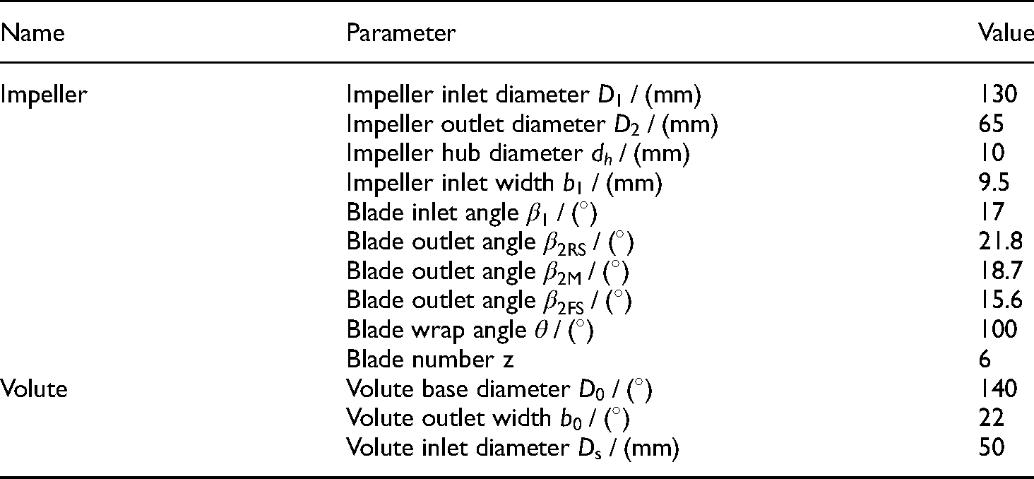
In Table 1,

The twisted blade structure and the computational fluid domain of PAT: (a) The blade angle of twisted blade; (b) computational fluid domain of PAT.
From Figure 1, the computational fluid domain includes import extension section, volute, impeller, and export extension section. As shown by the arrow, the liquid flows in through the inlet, then flows through the import extension, volute, impeller, export extension, and finally flows out through the outlet. In the numerical calculation, because the operating conditions of PAT are known, the boundary conditions of velocity inlet, free outflow and no-slip wall were adopted. The computational fluid domain includes static region and rotating region, the multiple reference frame (MRF) model was used to deal with this situation, the computational domain formed by the impeller was set as the rotating region, and the interfaces were used between the static-static and dynamic-static computational domains to transfer the computational data.
The SST 


where S is the absolute value of vorticity, 
The closure coefficients of equations (1) and (2) are as follows:
Grid independence check
The computational fluid domain was divided into structured grid. The block, mesh generation, refinement and grid independence check of computational fluid domain are shown in Figure 2. From Figure 2(a), because of the existence of triangular area in the impeller inlet and outlet of a single impeller channel, it is necessary to carry out Y-type segmentation for the two blocks. It is worth noting that because the cross sections of the import extension, the export extension and the volute are circular or quasi circular, the fluid domain structure of these three parts are segmented by O-type to improve the mesh quality, as shown in Figure 2(b) and (c). Since the division method of import extension and export extension is the same, the meshes of import extension are not shown in Figure 2(c). Based on the meshing of computational fluid domain, the efficiency of PAT was taken as the variable, and the number of grids was taken as the independent variable to check the grid independence. The result of grid independence check is shown in Figure 2(d). As can be seen from Figure 2(d), the efficiency of PAT increases with the increase of grid number. When the grid number changes from 913,058 to 1,029,816, the efficiency of PAT is basically at a constant value, so the final grid number is 1,029,816. In order to capture the flow state more clearly in the near wall area of the blade before and after optimization, the grids checked for independence were refined in the near wall area with d = 0.2 mm (the distance from the first layer grid node to the wall is 0.2 mm), 28 as shown in Figure 2(c).

Computational domain meshing of PAT flow field: (a) The block and meshing of single impeller channel; (b) The block of volute; (c) computational fluid domain meshing and refinement of PAT; (d) grid independence check.
Accuracy verification of numerical simulation
The structural diagram and the test site of the accuracy verification test system for the optimization results and numerical simulation of the PAT blade are shown in Figure 3. From Figure 3, the working principle of the PAT test system is as follows:

Accuracy verification test system for PAT numerical simulation: (a) The structural diagram of the accuracy verification test system; (b) The test site of the accuracy verification test system.
The water feed pump is driven by an electric motor to provide fluid with a certain pressure for the PAT test An electromagnetic flowmeter is installed on the pipeline between the water feed pump and the PAT to measure the flow through the PAT. The rated working pressure is
Numerical simulation and experiment were carried out on the prototype PAT to obtain the comparison diagrams of the external characteristic curves, as shown in Figure 4.
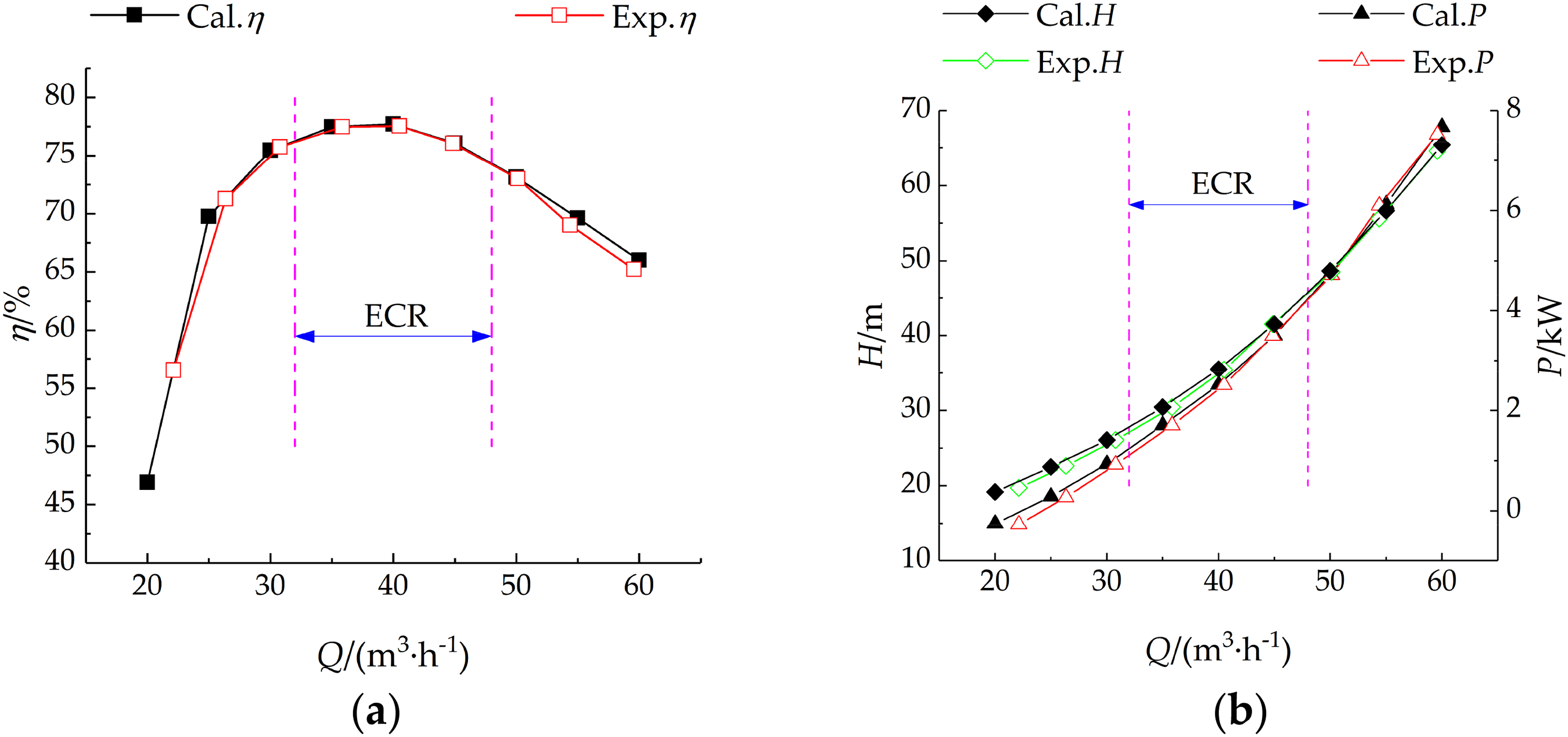
Numerical simulation and experimental external characteristic curves of prototype PAT: (a) flow-efficiency curves of PAT; (b) flow-power curves and flow-head curves of PAT.
It can be seen from Figure 4 that the trend of the external characteristic curves obtained by numerical simulation are basically consistent with that obtained by experiment. From Figure 4(a), there is a big difference between the small flow area and the large flow area, which is mainly caused by the low accuracy of the turbulence model for the flow simulation with separation and high reverse pressure gradient. It is generally considered that the error controllable region (ECR) is 0.8Q-1.2Q (the middle part of the two dotted lines in the Figure 4), 29 and the error at the optimal operating point is the smallest
Parameterization of twisted blade of PAT
The shape of twisted blade of PAT is at least formed by three blade profiles of FS, middle and RS. 30 Therefore, the shape of blade profile is very important for improving the performance of impeller. This also attributes the optimization of twisted blade to the optimization of three blade profiles, and the forming principle from blade profile to twisted blade surface determines the speed of blade modeling. The spatial blade profiles corresponding to the twisted blade of PAT and the forming method of twisted blade are shown in Figure 5.
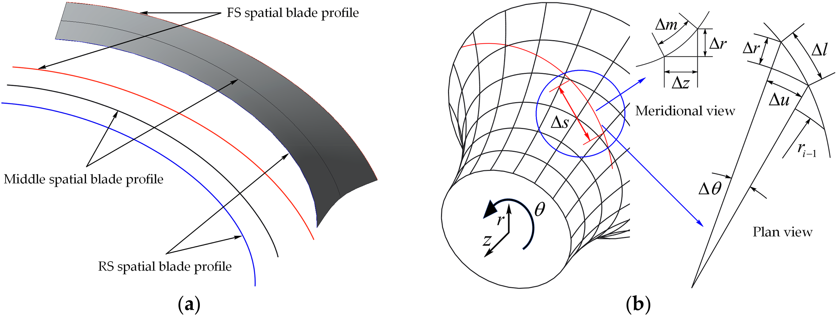
Drawing principle of twisted blade of PAT: (a) twisted blade and blade profiles; (b) drawing principle of twisted blade.
In the Figure 5(b),

Parameterization of PAT blade profiles: (a) expanded plan of PAT blade profiles; (b) parameterization of blade profiles. BP: Blade profile; BPCPL: Blade profile control point line.
From Figure 6(b), the shape of each blade profile is controlled by five control points, and three independent variables can be determined. It is specified that the independent variables change along the angle bisector of the included angle of the control line, and the included angle increases to positive and decreases to negative. The nine independent variables determined by the three twisted blade profiles and their value ranges are shown in Table 2.
Variable optimum interval of blade profile.

Optimization method and strategy
SVM-HDMR surrogate model theory
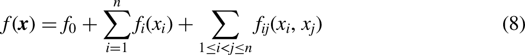
The construction idea of SVM-HDMR surrogate model can be described as follows: First, according to the HDMR theory,31–33 the output 


Finally, according to the SVM theory,37,38 when the model training set is linear or approximately linear, the regression function can be constructed as follows:


The construction process of PAT surrogate model. CFD: Computational fluid dynamics.
Objective function and optimization strategy
Through the analysis of the PAT surrogate model function, the optimization problem of the maximum value of the objective function can be described as follows: Step 1. According to the coordinates of each point of twisted blade of PAT, the twisted blade is represented by three blade profiles of FS, Middle and RS by Creo 3.0 and CFturbo 2020 software. Step 2. Three blade profiles are parameterized by Bezier curve with MATLAB 9.7 software programming function, and the training set of SVM-HDMR surrogate model is separated. Step 3. According to the separated training set of surrogate model, and the construction process of PAT SVM-HDMR surrogate model shown in Figure 7, the surrogate model function based on PAT efficiency is constructed by comprehensively using MATLAB 9.7, CFturbo 2020 and Fluent 19.2 software. Step 4. Genetic algorithm is used to search the surrogate model function globally in the optimization interval on the MATLAB 9.7 software platform, and the parameters of three blade profiles are fed back according to the optimization results.
When the surrogate model function obtains the optimal solution in the optimization interval, the optimization process ends. The three optimized blade profiles are modeled by CFturbo 2020 software, and the optimization results of the surrogate model are verified by numerical simulation. Experiment is conducted to verify the effectiveness of the optimization results and numerical simulation. When the surrogate model function obtains the optimal solution at the boundary of the optimization interval, it is necessary to repeat steps (3)–(4) based on the optimization result until the conditions of the end of the optimization process are satisfied.
Process, results, and discussion
The construction process of PAT surrogate model
According to the function characteristics of SVM-HDMR surrogate model, at least three function values are needed to determine a first order SVM-HDMR function besides the prototype model, that is, two efficiency values of PAT hydraulic model with single independent variable change are needed. To determine a second order SVM-HDMR function, at least five function values are needed, that is, four efficiency values of PAT hydraulic model with two independent variables changing each other are needed.
The first order and second order SVM-HDMR function terms constructed when the blade profile of the FS changes is taken as examples. MATLAB 9.7 software was used to generate Bezier curve of blade profile corresponding to the change of independent variables
Training point of surrogate model and efficiency of PAT.
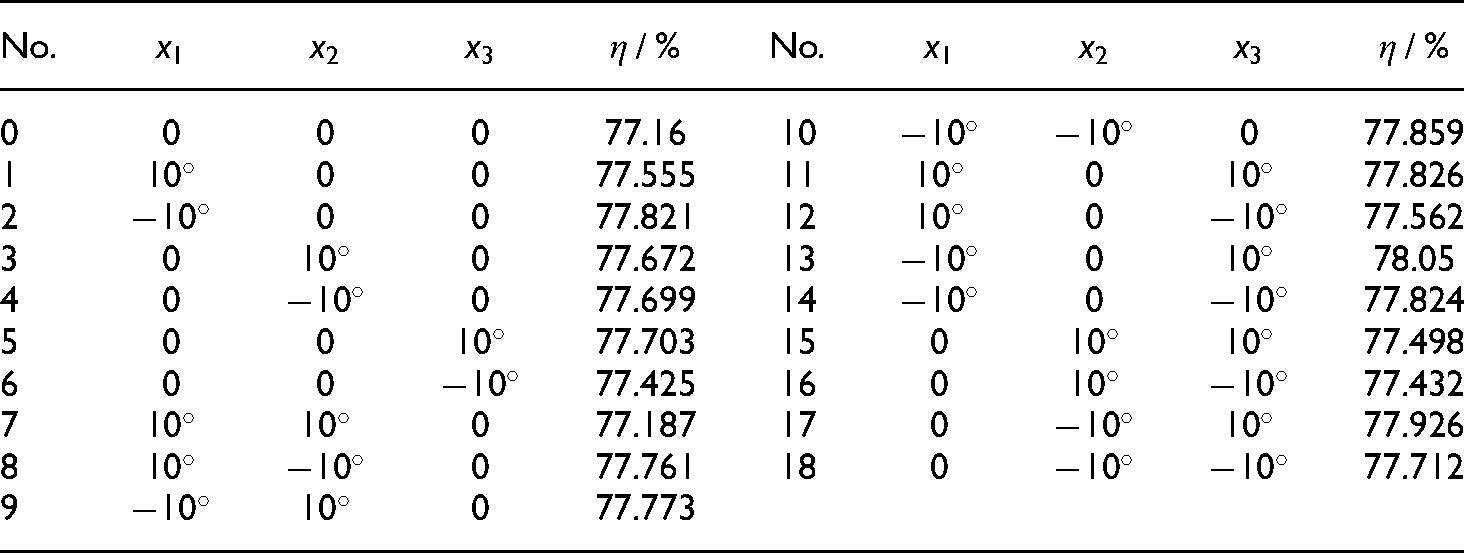
The model number 0 represents the prototype model, and the model number 1-18 is the corresponding PAT model formed when the independent variables

The first order and second order SVM-HDMR function terms determined by FS: (a)
Optimization results of PAT surrogate model
The function terms of the middle and the RS blade profile were constructed in the same way. In this way, after learning 55 PAT hydraulic models, the SVM-HDMR surrogate model function

Comparison of PAT blade profiles and corresponding twisted blade before and after optimization: (a) comparison of FS blade profile; (b) comparison of middle blade profile; (c) comparison of RS blade profile; (d) comparison of three-dimensional spatial blade profile; (e) comparison of three-dimensional twisted blade; (f) comparison of twisted blade impeller for test BP: blade profile; BPCPL: blade profile control point line; SBP: spatial blade profile.
Figure 9(a)–(c) are the comparison diagrams of blade profiles changes of FS, middle and RS before and after optimization. Figure 9(d) is the comparison diagram of three-dimensional PAT twisted blade spatial blade profile before and after optimization. Figure 9(e) is the comparison diagram of three-dimensional PAT twisted blade before and after optimization (FS is included in the diagram for comparison). Figure 9(f) is the comparison diagram of the corresponding PAT twisted blade impeller for test before and after optimization. From Figure 9(a), the optimized PAT blade profile on the FS side has no obvious change at the blade inlet (the outlet of the centrifugal pump blade), which is shown in the comparison diagram of the three-dimensional blade in Figure 9(e), and there is a staggered zone at the inlet of the PAT blade on the FS side (area A in the Figure 9(e)). From Figure 9(a)–(c), the bending degree of the optimized twisted blade is smaller on the FS side, and the variation of blade profile from FS to RS increases gradually. From Figure 9(d), the variation law of the three-dimensional spatial blade profile of the twisted blade is consistent with that shown in Figure 9(a)–(c). From Figure 9(e), the offset of optimized PAT twisted blade on RS side is more than 1.5 blade thickness (area B in the Figure 9(e)).
Flow field analysis
In order to analyze the change of fluid flow state in the impeller before and after blade optimization, the surface streamline diagrams of Z = 0, Z = 6 mm and Z = 17 mm before and after blade optimization were drawn, as shown in Figure 10.

Comparison of surface velocity streamline diagrams before and after impeller optimization: (a) Z = 0 plane; (b) Z = 6 mm plane; (c) Z = 17 mm plane.
The (1)–(3) in Figure 10 respectively represent the positions of each streamline plane in the impeller, the streamline diagrams of each surface before blade optimization and the streamline diagrams of each surface after blade optimization. From Figure 10(a) (2)–(3), the changes of flow conditions in the impeller before and after blade optimization mainly occur at the blade inlet (area C in the Figure 10(a) (2)) and blade outlet (area D in the Figure 10(a) (2)). Although the flow after optimization is more orderly, it is not obvious. From Figure 10(b) (2)–(3), the impeller before blade optimization has a flow separation zone at the blade outlet (area E in the Figure 10(b) (2)). After the fluid flows out of the blade area, there is an obvious velocity boundary (area F in the Figure 10(b) (2)). The existence of the separation zone weakens the work ability of the blade, and the existence of the velocity boundary increases the flow loss. From Figure 10(c) (2)–(3), when the fluid flows to the outlet of the impeller, there are obvious differences in the velocity size at the same radius, and there are different directions in the velocity at different radii of the same axial plane. The differences have disappeared in the impeller after blade optimization.
The twisted blade impeller before and after optimization was numerically simulated at the design operating point, and the process of fluid energy conversion and transportation in the impeller was analyzed by combining with the kinetic energy equation of viscous fluid.
40
The kinetic energy equation of steady incompressible fluid can be written as follows:
The first term at the right end of the formula is the work done by the body force to the fluid of unit mass in unit time. The body force includes gravity, electromagnetic force, etc., which will not be discussed here. The cloud images of the other terms at the right end of the formula and the left term of the formula at the plane with the axial coordinate of Z = -2.1 mm (the PAT impeller inlet width is 9.5 mm, PAT blade outlet position is Z = -2.4mm,and the cloud forming plane is close to the RS) are shown in Figure 11.

Comparison of cloud images of the formula before and after impeller optimization: (a) comparison of viscous transport term field; (b) comparison of flow work field; (c) comparison of dissipative term field; (d) comparison of convective transport term field.
Figure 11 (1) represent the internal flow cloud chart of the prototype PAT impeller, and Figure 11 (2) represent the internal flow cloud chart of the optimized impeller. The second term at the right end of the formula is the mechanical energy transported by the viscous force to the moving unit mass fluid in unit time, which represents the ability of the viscous force to change the spatial distribution of energy in the impeller. From Figure 11(a), under the same conditions, the internal transport intensity of the optimized impeller is weakened. The third term at the right end of the formula is the work done by the pressure per unit time to the fluid per unit mass, that is, the flow work. From Figure 11(b) (1)–(2), this term mainly acts on the blade inlet. From Figure 11(b), under the same conditions, the high intensity area of the optimized impeller cloud distribution is significantly reduced. The fourth term at the right end of the formula is the deformation work done by the viscous force per unit time, which is essentially different from other terms. By expanding this term, it is always positive, which means that at any position in the impeller space, some of the energy of fluid motion is converted into heat energy and dissipated, also known as the dissipation term. From Figure 11(c), under the same conditions, the area of high dissipation intensity of the optimized impeller is obviously reduced, which shows that the loss of the optimized impeller in the process of energy conversion is small. The left term of the formula is the convective transport term of kinetic energy. From Figure 11(d), under the same conditions, the transport intensity is obviously weakened, and the high-intensity region of transport is obviously reduced. It indicates that the amount of energy converted from kinetic energy to pressure energy will decrease, which indirectly indicates that the final viscous dissipation caused by transport in the impeller will decrease, represents the enhancement of the impeller's ability to do work on liquid.
In summary, the analysis of Figure 11(a), (b) and (d) show that the energy transport strength of the twisted blade impeller is weakened after optimization, which confirms the reduction of energy dissipation in the middle wheel of Figure 11(c). It indicates that the twisted blade impeller is more favorable for the transformation of fluid energy.
Verification of optimization results
The optimized PAT was numerically simulated and verified on the experimental equipment in Figure 3. The flow-efficiency, flow-head, and flow-power performance curves of the PAT before and after optimization were drawn, as shown in Figure 12.
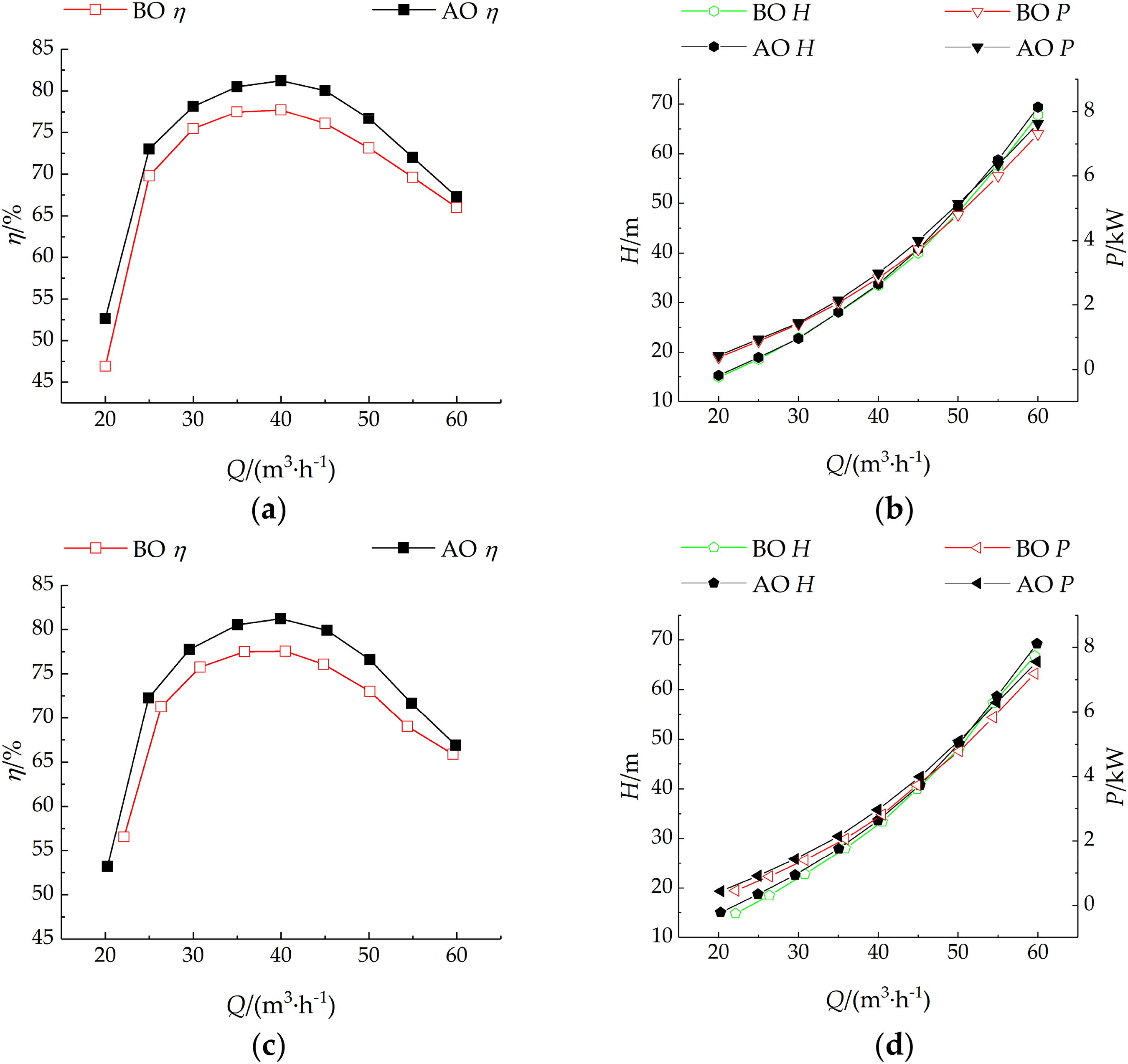
Performance curves of PAT: (a) flow-efficiency comparison diagram obtained by numerical simulation; (b) flow-power and flow-head comparison diagram obtained by numerical simulation; (c) flow-efficiency comparison diagram obtained by test; (d) flow-power and flow-head comparison diagram obtained by test BO: before optimization; AO: after optimization.
Figure 12(a) and (b) are the comparison diagrams of performance curves of PAT obtained by numerical simulation. Figure 12(c) and (d) are the comparison diagrams of performance curves of PAT obtained through test From Figure 12(a)–(c), the numerical simulation results are basically consistent with the experimental results. From Figure 12(a), the efficiency of the optimized PAT at the design operating point is 3.51% higher than that before optimization. From Figure 12(b), under design condition, the shaft power of the optimized PAT is increased by 5.3% compared with that before optimization. From Figure 12(c), the test efficiency of the optimized PAT at the design operating point is 3.4% higher than that before optimization. From Figure 12(d), the test output power of the optimized PAT at the design operating point is increased by 5.1% compared with that before optimization.
Conclusions
By redefining the variable of twisted blade profile to meet the condition of rapid modeling, the optimization of twisted blade of PAT was completed by using SVM-HDMR surrogate model combined with genetic algorithm. The optimization results were analyzed by using the velocity streamline diagram and the cloud diagram formed by kinetic energy equation. The optimization results were verified by numerical simulation and experiment. The following conclusions are drawn:
Comparing the velocity streamlines of the impeller before and after optimization, the flow field of the optimized impeller has obviously improved at the outlet of the blade. From the view of kinetic energy equation, the energy transport intensity of the optimized impeller is weakened, which indicates that the optimized impeller is more conducive to energy conversion. The optimization results are verified by numerical simulation. The results show that the simulation efficiency of the PAT after optimization at the design operating point is 3.51% higher than the efficiency of the PAT before optimization, and the output power is increased by 5.3%. The optimization results are verified by experiment. The results show that the results of numerical simulation and experiment are basically consistent. The test efficiency of the PAT after optimization at the design operating point is 3.4% higher than the efficiency of the PAT before optimization, and the output power is increased by 5.1%.
Footnotes
Declaration of Conflicting Interests
The author(s) declared no potential conflicts of interest with respect to the research, authorship, and/or publication of this article.
Funding
The author(s) disclosed receipt of the following financial support for the research, authorship, and/or publication of this article: This work was supported by the National Natural Science Foundation of China, Grant NO. 52169019; Industrial Support Program of Colleges in Gansu Province, Grant NO. 2020C-20; Gansu Outstanding Youth Fund, Grant NO. 20JR10RA203; Open Fund of Key Laboratory of Fluid and Power Machinery, Ministry of Education, Xihua University, Grant NO. szjj2019-016.