Sage Journals: Discover world-class research

Abstract

Introduction:

This preliminary assessment of a grey-box model, was predicated on system dynamics principles and developed using Vensim^® DSS software. The purpose is to predict biogas production under anaerobic conditions for energy utilization at the design stage.

Objective:

To describe the process of a developed system dynamics model to predict biogas production under anaerobic conditions.

Methods:

This method involves two-stage kinetics of the biogas production process in anaerobic conditions using the first-order and Gompertz functions. The model is depicted in two parts: causal loop diagram and stock–flow diagram. The causal loop diagram describes the anaerobic digestion process a substrate undergoes for the production of biogas, while stock–flow diagram depicts basic building blocks of the dynamic behavior of an anaerobic digestion process. Primary data is from a laboratory-scale experiment of biogas production using vegetal wastes, while the secondary one is from the literature on studies using similar substrates.

Results:

Primary and secondary data are used to validate and stimulate the developed model. The kinetic model shows the substrate being reduced exponentially with increasing time; consumption of substrate and production of methane and carbon dioxide follows exponential growth and decay pattern, with carbon dioxide production starting early compared to methane, and was produced at a rate faster due to the strong and resilient characteristics of fermentative microorganisms.

Discussion:

Comparing data from empirical and model simulation shows some close relationship, though not too perfectly. Both results reflect signs of inhibitions occurring within the substrates in the digester under anaerobic conditions explaining the low methane yield or instability.

Keywords

Kinetics biogas system dynamics growth function waste management

Introduction

A current trend of high dependence on biomass in Nigeria's energy consumption could be explored to reduce a considerable amount of waste generated from crop and livestock sectors of the economy. This is because the use of biomass for energy generation is sustainable and economical, viable financially, and benign to the environment.¹ The candidacy of biomass presents the best option amongst all available renewable energy resources; it is the most easily accessible source of energy with its unique environmentally friendly nature, constant supply, wider availability, and ease of integration into existing infrastructure.²

Anaerobic digestion (AD), gasification, thermal depolymerization, pyrolysis, fermentation, amongst others³ are existing technologies through which biomass could be converted for energy generation. AD is recognized as one of the best options for treating biomass as it helps to avoid carbon dioxide (CO₂) emissions and runoff of biomass.^4–6 It is a series of sequential natural processes, namely, hydrolysis, acidogenesis, acetogenesis, and methanogenesis^5,7,8 in which bacteria convert organic materials into biogas and fertilizer production in an environmentally friendly way. Though its underlying theory is well established, to further increase its value, it is important to research how AD could be optimized under diverse digestion conditions.⁹ We posit that optimization through computer-aided modeling of AD to examine the operating parameters to enhance its deployment and process efficiency is possible. A study,¹⁰ for instance, presents a dynamic model of biogas production systems based on system dynamics methodology but based on equations from the Gompertz model. Similarly, Pham Van et al.¹¹ studied the kinetic parameters of biogas production from co-digestion by batch mode without considering the effect of inhibition. These gaps were identified, hence our study on describing a developed system dynamics (SD) model to predict biogas production in AD based on the Gompertz model. It also scaled up the empirical data of biogas production to a pilot-scale biogas production taking into consideration the inhibitory tendencies within the substrates used in the laboratory experiment.

SD is a computer-aided approach to policy analysis and design that applies to problems arising in complex social, managerial, economic, or ecological systems.¹² Biogas production has both economic and ecological implications as it is one of the human demands for the provisioning services from the ecosystem. There is the need to examine these systems in an integrated manner to understand how trade-offs in their generation could be achieved. Ecosystems provide a wide range of services that are of fundamental importance to the well-being, health, subsistence, and survival of human beings.¹³ One of such impacts is the waste generated by confined animals, which can degrade the ecosystem and reduce the services it can supply.^14–16 A major means of handling this menace in the ecosystem is to use the wastes to generate energy in form of biogas. This approach means the production of energy from wastes as a provisioning service and, an ecosystem regulating service, as it mitigates undesirable effects in the environment.¹³ SD model is characterized by interdependence, mutual interaction, information feedback, and circular causality.¹² They are built around a particular problem, which in this study, is the effect of managing vegetal wastes in the economy and ecological systems. The relevant variables are drawn around this problem and are included in the model, to generate the model's boundary. Being a preliminary assessment, the SD model could be easily extended or revised to address additional questions as they arise. The study then is a description of how the SD model was developed to predict biogas production from vegetal wastes in anaerobic conditions. This preliminary assessment leveraged three sources of information namely, numerical data, written database (publications and operations manuals) of how the system works, as well as authors’ expert knowledge.¹²

The study objective is “to describe the process of a developed SD model of two-stage kinetics for predicting biogas production from any digester operating under anaerobic conditions.” The use of SD modeling is predicated on knowing that the approach is an excellent tool to study the kinetics of biogas production in anaerobic conditions as a closed-loop system. The anaerobic condition could be converted into information that can be observed and acted upon to change the initial condition.¹⁷

Literature review

Few kinds of research have been reported on the dynamic behavior of biogas production systems in modeling and simulation. This has been attributed to the complexities and complications involved in biogas production systems.^10,18–19 In the context of this study, few such kinds of research are reviewed as regards the mechanisms behind the AD process. For instance, a study of augmented AD Model No. 1 (ADM1) as a standard kinetic model of AD that is coupled to flux-balance-analysis (FBA) models of methanogenic species.¹⁸ It describes steady-state results of coupled models, that could provide detailed predictions on the intracellular activity of microbial species which are compatible with experimental data on enzyme synthesis activity or abundance as obtained by metatranscriptomics or metaproteomics. The study shows that by providing predictions of intracellular fluxes of individual community members, the approach advanced the simulation of microbial community-driven processes and provides a direct link to validation by state-of-the-art experimental techniques. Hamawand and Baillie¹⁹ describe a simulation to test the capability of software to predict biogas potential for two different anaerobic systems, namely, a laboratory-scale batch reactor and an industrial-scale anaerobic continuous lagoon digester. The software used data related to the operating conditions, the reactor design parameters, and the chemical properties of influent wastewater, with a sensitivity analysis done to identify the sensitivity of the most important default parameters in the software's models. The results from the software show that it could be used reliably to simulate both small-scale batch reactors and industrial-scale digesters. Bala and Satter¹⁰ and Fang et al.²⁰ report on the SD study of biogas production, positing that SD is the simplest and quickest route to the understanding of dynamic systems such as biogas production systems through models. It is capable of incorporating inherent nonlinearity and time lag of the system.^10,20 In a similar vein, Gavala et al.²¹ state that kinetic models are useful tools to optimize the AD process in SD. It is also reported that the kinetic of biomethanation helps in understanding the mechanisms of the AD process.^22,23 Pham Van et al.,²⁴ Deepanray et al.,²⁵ and Kythreotou et al.²⁶ report research that have deeply studied the influences of physical and chemical conditions on AD of a substrate. These influences have been modeled by different kinds of kinetic models including the kinetics of substrate degradation, growth kinetics, and kinetics of biogas production.^24–27 Kythreotou et al.²⁶ and Nopharatana et al.²⁷ also report that the kinetic model of biogas production was found to be the most important. Also, it is noted that there are some examples of non-dynamic white-box models based on stoichiometry and applied only for calculating biogas production.²⁸ These include models of Amon et al.,^29,30 Boyle,³¹ and Buswell and Mueller.³² These models are time-independent models, relying on data for basic elements or components of organic substrates. Such models become helpful for the estimation of values CH₄ and CO_2.³³

Models are either suitable for qualitative description or quantitative predictions.^28,34 In terms of the quantitative description, biogas models can be categorized as theoretical and experimental models.²⁸ Theoretical models, also known as first-order models, explains how a system works based on theoretical knowledge and predict system behavior.^35,36 On the other hand, experimental (empirical) models are models used to investigate the relationship between different parameters by carrying out tests on them. Empirical models are well known for validating a specific system for which it was developed while first-order models are known for their high predictive power.³⁷

Further categorization of models is that they can be referred to as white-box, grey-box, and black-box models, respectively.^38,39 White-box models usually will be such that would include the details needed in explaining the biochemical reactions in the AD process and they are also deductive. On the flip side is that black-box models exclude any prior information about the process and join the input with output inductively. Grey-box models involve the calculation by estimation procedure of parameters with physical interpretation and some approximation as well as simplification of the AD process. It has been reported that most dynamic models have a grey-box structure.⁴⁰ The SD kinetic model described in this study is grey-box, based on the parameters of the stock (biomass) used, the technology (AD), and the principle (SD) upon which the model was developed.

Laboratory experimental setup

The details of the laboratory experiment scaled up in this study are reported by Momodu et al.⁴¹ A brief description of the various steps employed during the laboratory experiment, including materials, digester design, feedstock sample collection and analysis, preparation of feedstock, digester setup, biogas collection, and analysis is here reported.

The materials include vegetal matter (vegetables and fruits), inoculum (cow rumen fluid), three 20-liter (0.02 m³) water jars of dimension, six 5-liter (0.005 m³) kegs, ¾ inch polyvinyl chloride (PVC) pipe, ¾ inch PVC pipe caps, length of tubes, funnel, calibrated cylinder for measurement, black polyethylene, paintbrush, clean water, glue, thermometer, and hand gloves. The equipment used for this project were OHAUS Adventurer Pro AV264 digital weigh balance, furnace, and Fourier transforms mid-infrared spectroscopy Shimadzu model (FTIR).

Three portable digesters were fabricated by adapting and modifying a 20-liter plastic container and using a 1-inch diameter PVC pipe. This was cut to 19.7 inches and placed through the bored hole until about 2 inches from the base of the plastic container (digester) and capped as the inlet pipe. A second hole was bored at the opposite side of the inlet pipe where the ½-inch diameter PVC pipe was inserted and capped as the outlet pipe through which samples were collected for pH analysis. The PVC pipes were tightened using epoxy glue so as to prevent leakages. The inlet and outlet pipes positions were connected to the gas storage capacity of a dome-shaped biodigester because the gas will be stored above the slurry.⁴²

A gas tube for the passage of gas was inserted into the neck of the biodigester by boring a hole and tightened using epoxy glue. The digesters were subsequently wrapped with black polyethylene to screen out light in order to avoid algae formation and to enhance methane production. In the presence of algae, oxygen will be produced; the bacteria will respire aerobically and methane gas will not be produced. Therefore, it is necessary to wrap the digester with black polyethylene to maintain the digester temperature. Water displacement method⁴³ was adopted for the gas collection by modifying the six 5-liter kegs as water tanks and collectors, implying that the volume of water displaced equals to the volume of gas produced. The digesters, water tanks, and water collectors were inter-connected using rubber hoses. A mechanical stirrer was not included in the design so as to avoid the problem of gas leakages. Stirring was done by shaking the biodigester to prevent thickening and settling of the slurry which is referred to as the dead zone within the digester.⁴⁴

In the framework of the experimental study, fruits and vegetable wastes were collected from a local food market. It was basically composed of a fresh waste sample of vegetables and fruits from various vegetable stalls at a market. The mixtures of vegetables and fruits used were composed of watermelon, tomatoes, and oranges. After the collection process, the vegetable and fruit wastes were grinded in order to increase the surface area. The considered inoculum was cow rumen fluid collected from a cow abattoir. Firstly, the cow rumen fluid was packed into polyethylene bags and stored at room temperature for four days before use so as to allow the production of more methanogens.⁴⁵ Secondly, the substrates were grinded using mortar and pestle to reduce and homogenize their sizes. Thirdly, the prepared substrate with cow rumen fluid were mixed together. The fourth step was to mix the slurry formed with water in the biodigester.⁴⁶

Total solid content, volatile solid (VS) content, biochemical methane potential was determined in accordance with the standard methods.⁴⁷

Three identical biodigesters were set up. Fresh vegetal wastes (V) which contain an equal volume of watermelons, tomatoes, and citrus were assigned to each biodigester, respectively, and mixed with cow rumen fluid (R) and clean water (W) into different V: W: R ratios; (1: 1: 0) control; (0.75:1:0.25); and (0.5:1:0.5) that correspond to 0%; 25%; 50% of rumen fluid, respectively (see Table 1). The retention time for each of them was 30 days. The mode of feeding of the digester was batch feeding; that is, loading the digester once and maintaining a closed environment throughout the retention period. The digester setup is shown in Plate 1.

Plate 1.

Laboratory experiment.

Table 1.

Conditions of the three different V:W:R ratio contents used for model simulation.

Biodigester	V:W:R ratio	Vegetal matter (g)	Water (mL)	Cow rumen fluid (mL)
D1	1:1:0	4000	2000	0
D2	0.75:1:0.25	3000	1500	1500
D3	0.5:1:0.5	5000	1000	3000

To improve the gas produced in the biodigester from the substrate, there was the addition of inoculum. This involved the introduction of cow rumen fluid as inoculum to the substrate. Other parameters that may affect this process such as ambient temperature, hydraulic retention time (HRT), organic loading rate (OLR), particle size, and nutrients were kept constant. The fruit and vegetable wastes were mixed in a carbon to nitrogen ratio of 1.4:1 under the pH condition of 6–7.2. The substrate to inoculum ratio of the digesters was 1:0 for control; 0.75:0.25 and 0.5:0.5 that correspond to 0%; 25%; 50% of the inoculum.

The gas produced was accumulated in the upper part of the biodigester. Since the water displacement method was adopted for the gas collection (Figure 1), the volume of water displaced equals to the volume of gas produced.⁴³ The daily volume of biogas produced was measured and recorded.

Figure 1.

Causal diagram for an experimental biogas production system.¹²

Methodology

The methodology took cognizance of these three critical parameters—the stock, the technology, and the principle—in developing the computer-aided model to assess an optimized AD operational deployment and efficiency. These three parameters form the basis of the development of the two-stage kinetic model. It was approached at two scales—laboratory and field levels, respectively. Primary and secondary data were used to first validate the model, after which it was simulated to ascertain its functionality. The primary data were obtained from a laboratory experiment of biogas production using vegetal wastes while the secondary data were obtained from the literature of the same substrate types.

Future biogas plants would need to be designed to meet demand, through proactive feeding management.⁴⁸ This forms the basis of the design on which this simulation model was developed, not minding the substrate supplied. Most biogas production simulation processes are based on the complex ADM1, covering a large number of parameters for all biochemical and physicochemical process steps. These steps are carefully adjusted to represent the conditions of a respective full-scale biogas plant. However, reliable measurement technology and process monitoring are currently deficient, being nearly none available for full-scale plants. The laboratory experiment was conducted under three conditions depicted as Digester 1 (D1), Digester 2 (D2), and Digester 3 (D3), respectively. The conditions were based on fresh vegetal wastes (V) mixed with cow rumen fluid (R), and clean water (W) in different V:W:R ratios. The temperature at the mesophilic range was assumed to be constant in all three conditions for simulation purposes. The two-stage kinetic model was developed based on SD principles using Vensim^® software.

Conceptual framework of the model

As AD involves microbe growth processes, the concept of describing the study is that of growth processes.⁴⁹ Describing growth data usually resorts to 3-parameter families of curves, namely, the logistic, the Gompertz, the exponential, and the parabolic functions.⁵⁰ AD growth processes involving hydrolysis, acidogenesis, acetogenesis, and methanogenesis, are usually described using both the logistic and the Gompertz growth functions, respectively.⁵¹ Though the logistic has been more studied, it is the Gompertz growth function that is described as being better to meet the features of some growth processes.⁵¹ According to Vieira and Hoffmann,⁵¹ the equations describing each of these functions are given as follows:

Logistic growth function, Z = a / [1 + \exp {- (b + c t)}]

(1)

where a, b, and c are parameters, a \gt 0 and c \gt 0, and

Gompertz growth function, Z = \exp (a - b c t)

(2)

where a, b, and c are parameters, b > 0 and 0 < c < 1.

Both functions are monotonically increasing and lie between two asymptotes, which are Z = 0 and Z = a for function (1) and Z = 0 and Z = ea for function (2). Both functions have points of inflection whose co-ordinates are t = −b/c and Z = ½a for function (1) and t = −logb/logc and Z = e^a^−l for function (2). However, the logistic growth function has very peculiar features: for one, the location of the point of inflection is exactly halfway between the two asymptotes, and secondly, there is a radial symmetry with the point of inflection. According to Bain,⁵² the location of the point of inflection of the logistic function is a drawback for some purposes, and according to Pearl and Reed,⁵³ growth rates symmetric around the point of inflection are not realized in many growth processes. On the other hand, the ordinate of the point of inflection of the Gompertz growth function, although its value is also related to the asymptote, is relatively smaller than that of the logistic growth function and there is no symmetry involved. Thus, these features may better meet the characteristics of some growth processes. The logistic and the Gompertz functions are not easy to fit satisfactorily to actual data.⁵¹

Of course, there are some crude methods of estimation for both functions. A popular one consists of dividing the observed values into three equally sized groups, eliminating one or two observations if their number is not divisible by 3, averaging them, and solving the resulting three equations for the three parameters. According to Stevens,⁵⁴ the estimates obtained by this three-point method are consistent but very inefficient. An assumption concerning the error term involving heteroscedasticity may dictate transforming the function before estimating it. In the cases where the variances of logarithms of Z_i are constant, the Gompertz growth function should be fitted by the method proposed by Stevens⁵⁴ and the logistic growth function by the method proposed by Nelder.⁵⁵ However, when the variances of Z_i are constant, the logistic growth function should be fitted by the method proposed by Oliver⁵⁶ and the Gompertz growth function by the method.⁵¹

With this backdrop, knowing the models usually applied to capture the characteristics of the AD process such as the first-order model, logistic model, and Gompertz model,^11,57 the Gompertz model is considered as the best model.¹¹ Gompertz's model describes the growth of animals and plants as well as the volume of bacteria. There are two main types of the Gompertz model. These models vary depending on the number of parameters in the model. They include the four-parameter Gompertz, the Zwietering modification, the Zweifel and Lasker re-parameterization, the Gompertz-Laird, and the Unified-Gompertz.⁵⁸ Gompertz-Laird is one of the more commonly used. The Gompertz model describes the cumulative biogas production curve in batch digestion assuming that substrate levels limit growth in a logarithmic relationship.⁵⁹ The Gompertz model is given in the following equation:

G_{t} = A \times Exp {- \exp [\frac{μ_{m} \times \exp (1)}{A} (λ - t) + 1]}

(3)

where G_t is the accumulative biogas yield at digestion time t (Nml/g-VS), A is the biogas yield potential of the substrates (Nml/g-VS), μ_m is the maximum biogas production rate (Nml/g-VS), λ is the lag phase period or minimum time to produce biogas (day), and t is the digestion time (day). Also, when t = 0 then G(t = 0) is always more than zero, which means that this model always fails to describe at the starting time.

Although, in the Gompertz model, the parameter of the lag phase period (ƛ) was proved as a mathematical constant and not a biological one. This also implies that when time, t = 0, the Gompertz model will always fail to describe the starting time.²⁴ Therefore, to overcome this limitation, a new biogas production kinetic (BPK) model was proposed. This new model introduces meaningful parameters in biogas yield potential from substrates, these are µ_m and t_0, where μ_m is the maximum biogas production rate at t₀ and t₀ is the time when the gas production rate reaches the maximum value for simulation of biogas production, respectively.^58,59 This new model forms the basis for which the SD model was developed for this study.

The mathematical equation of the model

This study was based on the BPK model. In this model, two-level variables were developed using kinetic expressions describing the anaerobic process of the substrate. The first-level variable represents the first stage of the biogas production process, which is hydrolysis–acidogenesis while the second level variable is the second stage of the process, namely, acetogenesis–methanogenesis. The two stages of the biogas production process are defined, theoretically, by the same first-order equation, with their unique constants. The mathematical model is represented by the following equation²⁸:

\frac{d S}{d t} = (S_{0} - S) * D + (\frac{d S}{d t}) r

(4)

accumulation = input − output + reaction

where $d S / d t$ is the accumulation rate (change of the substrate concentration over change in time); D is the dilution rate (d⁻¹); S₀ is the initial substrate concentration; S is the substrate concentration; and, r is the reaction rate.

The equation shows two parts to the biogas production process: a technical part or mode of operation represented as (S₀– S)*D and a chemical part, depicted by $- (d S / d t) r$ . The technical part is responsible for the transition phase, input and output flows while the chemical part describes the dynamical change of the compound or substrate.

Model formulation

The SD model formulation involves the following processes: problem definition, identification of key variables which leads to the causal diagram, development of the model involving; reference mode development, and stock–flow diagram (SFD).⁶⁰ The SD model formulation is based on SD principles and developed on the Vensim DSS^® platform.

For the study, the problem definition involves the description of the kinetics of biogas production. The model developed seeks to express the kinetics of biogas production based on the SD approach. The two steps for SD model development are generating the causal and SFDs of the system being examined.

Causal loop diagramming (CLD)

The causal diagram helps, first, to describe the concept of the system, which in this case is the biogas production from the anaerobic process; and secondly, to identify the key variables that drive the system in the model. For this study, the process of generating the causal diagram of the anaerobic process led to the identification of all relevant parameters and influential variables used for this study. Figure 1 reflects the reviewed literature¹⁰ on biogas production. This diagram describes the AD process that a substrate will normally undergo for the production of biogas which includes: hydrolysis, acidogenesis, acetogenesis, and methanogenesis. The figure could also be used to explain the effect of inhibition that may likely occur during an AD process.^61,62

An example of inhibition as related to Figure 1 is described in Plate 2. Sun et al.⁶³ report that the microbiology of the AD process is predicated on several interdependencies permitting the conversion of a variety of complex organic materials to methane through the processes of hydrolysis, acidogenesis, acetogenesis, hydrogenogenesis, and methanogenesis.⁶⁴ According to Yangin-Gomec and Ozturk,⁶⁵ high protein content in the substrate releases ammonia when hydrolyzed, causing increased buffering capacity of the AD process, but with reduced overall C/N ratio^66,67 indicates that this can lead to operational difficulties through inhibition of the methanogenic microflora resulting from free ammonia accumulation in the digester (see Plate 1). This inhibition is reported at a wide range of total ammonia nitrogen (TAN) concentrations between 1500 and 7000 mg N L⁻¹.⁶² Sun et al.⁶³ stated that methanogenesis was completely inhibited at TAN of 9 g N L⁻¹. Digester failure due to ammonia inhibition is usually a result of the accumulation of volatile fatty acids (VFAs) to a point where the buffering capacity of the digester is broken and the pH falls to <6 with a corresponding loss of methane production and a reduction in the methane content of any biogas produced.^68,69 The suggested means of dealing with this inhibition caused by nitrogen-rich feedstock for AD include acclimatisation, trace element addition, dilution, and ammonia stripping.^70,71

Plate 2.

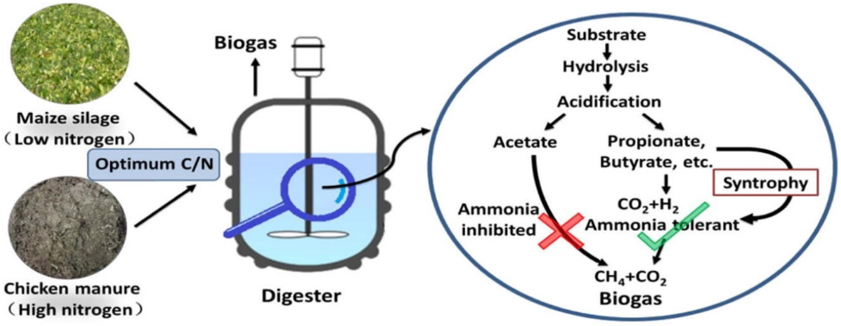
Describing inhibition effect on biogas production in a digester.⁷²

The causal diagram helps in the development of the reference mode in the model,⁶⁰ in this case, data from the laboratory experiment, supporting the translation of the dynamic behavior of the biogas production process into a graphical form. The dynamic behavior of the variables in the model was referenced against the experimental data to validate the model.

Stock–flow diagramming (SFD)

Stock and flow (or level and rate) diagrams are ways of representing the structure of a system with more detailed information than is shown in a causal loop diagram.⁷³ Stocks (levels) are fundamental to generating behavior in a system; flows (rates) cause stocks to change. Stock and flow diagrams are the most common first step in building a simulation model because they help define types of variables that are important in causing the behavior. Levels are also known as stocks, accumulations, or state variables. Levels change their values by accumulating or integrating rates. This means that the values of levels change continuously over time even when the rates are changing discontinuously. Rates, also known as flows, change the value of levels. The value of a rate is not dependent on previous values of that rate; instead, the levels in a system, along with exogenous influences, determine the values of rates. Intermediate concepts or calculations are known as auxiliaries and, like rates, can change immediately in response to changes in levels of exogenous influences. When constructing a level and rate diagram, consideration is given to what variables accumulate over some time. SFD is constructed based on knowing what levels are needed. This is first constructed and then the rates and auxiliaries are connected to it. It is important to note that model building is iterative. The rate has a single arrowhead, indicating the direction that material can flow (the rate can only increase the level). The SFD is only a diagram; in a simulation model, the equation governs the direction that material can flow (see Figure 2(a) and (b)). However, the diagram is used to indicate whether the flow is intended to be one way or two way.

Figure 2.

(a) Example of one-way stock–flow diagram and (b) example of two-way stock–flow diagram.

Equation driving the model simulations

Having described the mathematical representation of the study and also that of the SFD, this section focuses on the specific equations that govern the direction that materials would flow to in the two-level variables. The two-level variables represent hydrolysis–acidogenesis and acetogenesis–methanogenesis in the AD process. The level variable hydrolysis–acidogenesis is characterized by the hydrolysis rate constant (k), hydrolyzable rate of the substrate ( $α),$ expressed by the first-order kinetic model.

\frac{d C}{d t} = k \cdot (α \cdot C)

(5)

where C is the initial solid carbon and k is the hydrolysis rate constant.

The first-order model (equation (5)) and the Gompertz model (equation (6))¹¹ are applied to simulate the kinetics of biogas production.

G_{t =} A {1 - \exp [(m - 1) {(\frac{t}{t_{0}})}^{(\frac{1}{m})}]}

(6)

where G_t is the accumulative biogas yield at digestion time t; A is the biogas yield potential of substrates; m is an intermediate constant; t₀ is the time when the biogas rate reaches a maximum.

The kinetic average rate constant which quantifies the rate of a chemical equation could be obtained from the Gompertz model in equation (6).¹¹ The kinetic average constant, k is given as follows:

k = \frac{1}{m \cdot t_{0}} \cdot \exp (m) \cdot (1 - m)

(7)

For this study, equation (6) was modified into a simple form by the following equation:

G_{t} = A \cdot k

(8)

In the hydrolysis stage of an AD process, carbohydrates, fats, and proteins are all broken down into smaller molecules by this initial step of the process.⁶³ Acidogenic bacteria degrade the products of hydrolysis into volatile fatty acids. Some hydrogen, CO₂, and acetic acid (CH₃COOH), are also produced, which will skip the acetogenesis stage.⁶⁴

In the hydrolysis–acidogenesis stage of biogas production, CO₂ and hydrolyzable carbon are produced as indicated in the SDM. CO₂ is characterized by the kinetic average specific rate of digestion (KC1) and CO₂ potential of fermentation (AC1) while the hydrolyzable carbon which is characterized by hydrolysis rate constant, goes into the acetogenesis–methanogenesis stage.

The acetogenesis–methanogenesis stage is expressed in the SDM as an integral part of the output from hydrolyzable carbon.⁶⁵ This stage is where the methane and CO₂ produced in the AD process are captured. The output methane is characterized by the methane rate constant (km), methane potential (Am), and batch time while that of CO₂ is characterized by the kinetic average specific rate of digestion (KC1), CO₂ potential of fermentation (AC1), and CO₂ potential of methanogenesis (AC2). The total gas produced is the sum of the outputs (methane and CO₂).

Results and discussion

The study objective is to describe the process of a developed SD model of two-stage kinetics for predicting biogas production from any digester operating under anaerobic conditions. The ensuing activities were to: generate a causal loop and SFDs that represent the kinetics of the biogas production system, using SD principles to drive a Gompertz model for the system. Following the development of the model was its validation and then simulated to generate data that were compared with data obtained from the laboratory-scale experiment. This section describes and discusses the results obtained from the study.

Figure 3 describes the CLD generated from this study to show our understanding of the AD process that substrate undergoes for biogas production as earlier indicated. The figure contains 28 information links showing interconnection in a typical anaerobic digestion system. The first eight links on the substrate represent the factors that affect it in regards to biogas production in an anaerobic condition.⁶⁶ The substrate links to the hydrolysis stage which is the breaking down of the substrate into four different components (water, simple sugars, amino acids, and fatty acids) as shown by the information links in the diagram. This information link connects to the acidogenesis stage which is the second stage where acidogenic bacteria act on the product of the hydrolysis stage and convert them to CO₂, ammonia, and H₂S⁶⁷ as shown in the diagram. These links connect to the acetogenesis stage where CO₂, NH₃, and H₂S are acted upon by the acetogenic bacteria to produce acetic acids which lead to the methanogenesis stage. In the methanogenesis stage, methanogens metabolize the acetic acids into methane, CO₂, H₂S, and other trace gases which are the last three information links.⁶⁶ The description of this process depicts an ideal anaerobic condition that is not inhibited.⁶⁸

Figure 3.

Causal diagram of anaerobic digestion of substrate for biogas production.

Going back to Figure 1 as described earlier, where the anaerobic process exhibits two phases, namely, “growth” and “death” in the system.^10,70 The growth phase indicates a generation of positive feedback, which in the case of biogas production, could mean the absence of inhibitors⁶¹ in the biogas production process. The generation of negative feedback or counter-balancing effect implies attaining equilibrium in the system, which in respect to biogas production, signifies the death/decay phase where there could be inhibition. The inhibitors are principally ammonia and sulfate/sulfide.⁶⁸ During experimental research, the condition (pH, non-evacuating the gas)^70,71 in which the operated digester encouraged inhibition. Inhibition could occur in the biodigester for the following reasons: single daily evacuation, substrate exhibiting the presence of ammonia, sulfate, light metals, heavy metals, long-chain fatty acids, organics, and halogenated inorganic compounds in the digester (e.g. see, Sun et al.,⁶⁶ Yenigun and Demirel⁶⁷). The presence of inhibition affects the production of biogas leading to low methane yield or instability.⁶³ There are two major loops in Figure 1 describing the effect of acid and methane-forming bacteria respectively in the AD process. The two loops in the CLD represent two major phases in the biogas production process namely: hydrolysis–acidogenesis and acetogenesis–methanogenesis. These are distinctly represented as level variables in the SD model shown in Figure 4.

Figure 4.

System dynamics model (SDM) of biogas generation.

Validation and simulation of the SD model

The SFD and equations for the kinetics of the biogas production model have been described in the methodology section. This section describes the validation and simulation of the model. As will be seen better in the analysis, the model was validated using laboratory experimental data of biogas production obtained for 30-day retention time. To predict the production of biogas from any substrate, it is necessary to make use of the baseline information which are nutrient content, total and VSs content, chemical and biological oxygen demand, carbon/nitrogen ratio, and the presence of inhibitory substances. Key kinetic constants obtained from calibration and validation are k = 0.22; KC1 = 0.18; Kh = 0.22; and Km = 0.039.

In terms of the hydrolysis–acidogenesis stage, the simulation result from the first-order kinetic model exhibits an exponential reduction with progression in time,⁷⁴ as shown in Figure 5. The temperature has a significant influence on the production of biogas, with the digester temperatures range generally varying between 30°C and 39°C for daily readings, with an average of 36°C. This range conforms to the optimum range for mesophilic digestion (between 25°C and 38°C).⁷⁵ This is because, according to Donoso-Bravo et al.,⁷⁵ the anaerobes are most active in this mesophilic range. However, the slight daily variations noted in the readings could have contributed to inhibiting gas production as seen from the inconsistency demonstrated from the graph shown in Figure 6 for the three digesters. Temperature differences slow down the actions of methanogenic bacteria which are responsible for the production of methane.

Figure 5.

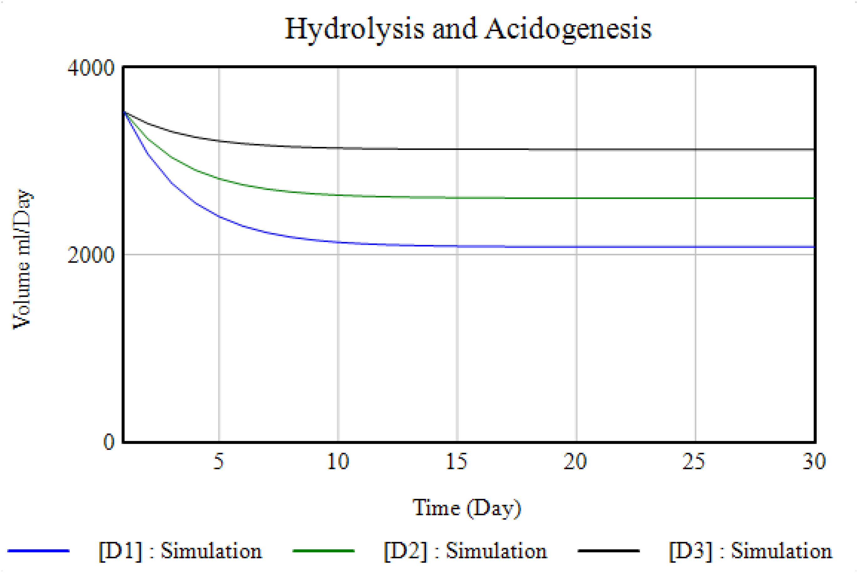
Kinetics of hydrolysis–acidogenesis.

Figure 6.

Volume of gas produced in laboratory-scale experiment.

The second aspect of the laboratory result of biogas production is that of the rumen. In general, biogas production rate tends to obey sigmoid function (S curve) as generally occurred in the batch growth curve. Biogas production is very slow at the beginning and at the end period of observation. This is predicted due to the biogas production rate in the batch condition is directly corresponding to a specific growth rate of methanogenic bacteria in the biodigester. During the first 10 days of observation, biogas production was very low or indeed do not produce due to the lag phase of microbial growth. In the range of 12–27 days observation, biogas production is significantly increased due to the exponential growth of microorganisms. After 27 days of observation, especially for substrate without rumen fluid (D1), biogas production tends to decrease and this is a predicted trend due to the stationary phase of microbial growth. After 27 days of observation, there was a tendency for an increase in biogas production for D2 and D3. This is predicted that the carbons contained by all waste constituents are not equally degraded or converted to biogas through AD. From Figure 6, it was observed that D2 and D3 exhibit higher biogas production than D1. The same behavior was also shown in the average biogas production curve. This result showed that the presence of liquid rumen in feed cause cumulative biogas production more than twice fold in comparison to feed without liquid rumen. This suggests that a high concentration of anaerobic bacteria content in liquid rumen works effectively to degrade organic substrate. According to Aurora,⁷⁶ rumen of the ruminant animals contains highly anaerobic bacteria dominated by cellulolytic bacteria able to biodegrade cellulose material from manure.

Figure 7 shows simulated data for methane and CO₂ produced during the retention time of 30 days. It could be observed that methane production of methane was higher than that of CO₂, even though CO₂ production is always ahead of methane in the biodigester. It could therefore be deduced that CO₂ started early compared to methane and got the maximum rate early because of the strong and resilient characteristics of fermentative microorganisms.⁷⁷ Figure 8 however, shows that the consumption of substrate and production of biogas follows more of exponential growth and decay pattern.⁷⁴ This situation depicts the characteristics of any dynamic process, involving accumulation and delay, such as biogas production in anaerobic conditions, growth, and decay is orchestrated through time. This growth and decay cause imbalances and cannot be explained solely by a causal link.⁷⁸ Accumulations change according to their inflows and outflows. Where the inflow is greater than the outflow the level will gradually rise, and where the outflow is greater than the inflow then the level gradually falls. In a similar vein, where the inflow and outflow are identical then the level remains constant. On the other hand, we observed that the model simulation result shows biogas production rate rising exponentially with progression in time, and after reaching a maximum point, and decreases continuously. Comparing this to the data obtained from the experimental data, indicating a significant lag phase or delay in biogas production occurred from between methanogenesis and fermentation stage as described by Boulanger et al.⁷⁹ It could be thus deduced that this lag phase or delay is orchestrated by the variation of dissolved organic carbon (DOC), which in turn is a result of the combination of two main phenomena.⁷⁹ The first of the two phenomena are that the hydrolysis of waste would lead to an increase in the DOC concentration, while the second is that the methanogenesis of acetate and H₂/CO₂, directly or indirectly contribute to the decrease of DOC concentration. The initial increase is attributed to the rapid hydrolysis of waste before the start of the active methane production phase. As active methanogenesis takes place, the DOC concentration decreases indicating the transfer of the organic carbon from the dissolved phase to the biogas. Consequently, methane production was slow and did not significantly deplete the accumulating DOC.

Figure 7.

Simulated data for methane and carbon dioxide production.

Figure 8.

Different gases were produced from the model simulation.

The model was validated using data obtained from a laboratory-scale experiment to produce biogas, depicted as Lab-Scale-Exp Data in the simulation of the SDM as shown in Figure 9. Figure 9 are the results for both simulated and laboratory experimental data of biogas produced. The laboratory experimental data used is that of D3 as shown in Figure 9, while the different conditions of D1, D2, and D3 were inputted into the model as subscripted values of rates for simulation. In the case of the laboratory-scale experiment, the effect of inhibition is clearly shown as the graph shows a lot of inconsistencies which could be attributed to some factors that increased acetoclastic activity, suggesting acetoclastic methanogens (and not hydrogenotrophic). This is limiting for the onset of the active methane production phase, causing the inhibition.⁸⁰

Figure 9.

Simulated and laboratory experimental data of biogas produced.

Anaerobic degradation is known to be a complex series/parallel reaction,⁸¹ usually subjected to various factors, such as inhibition. Although acetoclastic methanogenesis may not be the rate-limiting step in the anaerobic degradation of organics, especially of suspended solids, it is fingered as an inhibitor in the whole process of biogas production, because of the high fraction of COD (∼70%) converted by the acetoclastic methanogens.⁸² This event is very likely to occur when an inhibitor is added to the digester feed due to the high sensitivity of these methanogens to toxicants on the active biomass, particularly to halogenated organics.

Conditions of the substrate of data for the model simulation follow that used in the laboratory experiment (see Plate 1) as presented in Table 1. The temperature was assumed to be the same in all digesters when readings were taken.

Conclusions

The study conducted an assessment for predicting biogas production in anaerobic conditions. The approach is premised on first-order and Gompertz growth functions, respectively. These were built into SD-based model and developed using Vensim DSS^® software. The developed model is a grey-box model. The first was to develop the CLD to describe the process of an ideal anaerobic condition that is not exhibiting inhibitory tendencies, and secondly, the SFD that explains the dynamics of the process, incorporating both first-order and Gompertz functions in two-level variables. The third step was to validate the developed model using data obtained from biogas produced from a laboratory-scale experiment. The fourth step was a simulation, which shows results comparing data obtained from laboratory-scale experiments and that generated from simulating the modeling. The results exhibited differences, which could be adduced to inhibitory tendencies within the laboratory experimental data that affected the production of biogas leading to low methane yield or instability. This observation could be attributed to some factors that increased acetoclastic activity, suggest that acetoclastic methanogens (and not hydrogenotrophic) are limiting for the onset of the active methane production phase, causing the inhibition. However, these may need to be examined further, though, despite its grey behavior, there is the feasibility of using the BPK model to simulate the evolution of CO₂ and CH₄. Also, the model provided some vital information on the biogas production process, as it serves as a stepping stone to bridging the theoretical gap in BPK.

Footnotes

The authors thank the Centre for Energy Research and Development, CERD, OAU for access to facilities during the duration of this project. Also, the conduct of the research was encouraged through earlier support by funding from the Department for International Development (DfID) under the Climate Impact Research Capacity and Leadership Enhancement (CIRCLE) program. The funders had no role in study design, data collection, and analysis, decision to publish, or preparation of the manuscript.

Declaration of conflicting interests

The authors declared no potential conflicts of interest with respect to the research, authorship, and/or publication of this article.

Funding

The authors disclosed receipt of the following financial support for the research, authorship, and/or publication of this article: This work was supported by the Association of Commonwealth Universities (grant number Publication Fee).

ORCID iD

Abiodun S Momodu

Appendix 1

AC1 = 60.1; units: Nml/gVS

AC2 = 111.5; units: Nml/gVS

Acetogenesis and methanogenesis [inoculum = INTEG (hydrolyzable carbon [inoculum]−CH₄ [inoculum]−CO₂a [inoculum], hydrolyzable carbon [inoculum]); units: Dmnl

Alpha = 0.839; units: Dmnl

Am = 257.2; units: Nml/gVS

Batch time = 7; units: **undefined**

CH₄ [inoculum = DELAY3 (acetogenesis and methanogenesis [inoculum]/(Am*km), batch time); units: Nml/gVS

DELAY N (hydrolyzable carbon, (Am*km), batch time, 7)

CO₂ [inoculum] = hydrolysis [inoculum]/(kC1*AC1); units: Nml/gVS

CO_2a [inoculum] = acetogenesis and methanogenesis [inoculum]/(kC1*(AC1 + AC2)); units: Nml/gVS

Hydrolysis [inoculum] = INTEG (alpha*Substrate in[inoculum]−CO₂[inoculum]−hydrolyzable carbon[inoculum], Initial solid state of carbon [inoculum]); units: Dmnl

Hydrolysable carbon[inoculum] = hydrolysis[inoculum]*Kh; units: Dmnl

Initial solid state of carbon [inoculum] = 0.588*100; units: g

k = 0.22; units: Dmnl

KC1 = 0.18; units: Dmnl

Kh = 0.22; units: **undefined**

Km = 0.039; units: Dmnl

Ratio CO₂ to CH₄[inoculum] = CH₄[inoculum]/CO_2a[inoculum]; units: **undefined**

*Substrate in [inoculum] = (initial solid state of carbon[inoculum] + the inoculum[inoculum])*k; units: g

The inoculum [inoculum] = 0, 0.25, 0.5; units: **undefined**

where D1, D2, and D3 represent the percentage of inoculum to be added to the substrate in each digester, that is, 0%, 25%, and 50%, respectively. Inoculum used: cow rumen fluid.

Author biographies

Abiodun S Momodu holds a doctoral degree in Technology Management from Obafemi Awolowo University (OAU), Ile-Ife, Nigeria. He has been actively involved in policy and developmental research with particular emphasis on energy planning and environmental management, System Thinking, System Dynamics and modeling as well as S & T policy analysis since 2005. He has 15 years of professional experience being involved and leading energy and environmental research and analysis. He is currently the Head, Division of Energy Management and Technology, and is a senior research fellow at the Centre for Energy Research and Development, Obafemi Awolowo University, Ile-Ife, Nigeria. He did his postdoctoral fellowship at the Kwame Nkrumah University of Science and Technology, Kumasi, Ghana under the auspices of the African Academy of Sciences (AAS) in conjunction with the Association of Commonwealth Universities (ACU). He is also an associate lecturer at the Department of Agricultural and Environmental Engineering, OAU, Ile-Ife. His researches span energy planning and environmental management, with particular emphasis in electricity system and bioenergy, techno-policy analysis, climate change, gender and system thinking and modeling. He is a member of many learned professional bodies such as the System Dynamics Society (SDS), Nigerian Association of Energy Economics (NAEE) and an affiliate member of International Association of Energy Economics (IAEE). He has published over 30 articles in peer reviewed journals, aside from various technical reports. He is the head of the System Dynamics Research and Modeling Group at the CERD, OAU, Ile-Ife.

Tofunmi D Adepoju holds a first degree in Chemical Engineering from Obafemi Awolowo University (OAU), Ile-Ife Nigeria, with Second Class Honours (Upper Division). She graduated in 2019. Having concluded the compulsory National Youth Service, she proceeded to do her master of science degree in Technology Management, with research focus in bioenergy, converting wastes to energy. Her other areas of research interests include: waste management, climate change and system dynamics modelling. She is familiar with fundamental concepts of energy engineering, material sciences, transport phenomena, environmental management, and other fundamentals to energy management and engineering. She is also trained in health, safety and environment. She is trained in personal effectiveness, time management, effective communication, work etiquette, creativity and innovation, employability skills, emotional intelligence. She has interned with established researchers who have mentored her and has culminated in the publications in reputable journals. She is a has volunteered as social worker at Treasure Orphanage, Karu, Abuja, for International Youth Day, technical assistant in the following places: Community Excellence and Development Initiative (CEDI) Nigeria; System Dynamics Research and Modelling Group, Centre for Energy Research and Development (CERD), OAU, Ile-Ife, Nigeria. She has been involved in proposal writings with multi-disciplinarity.

References

US EPA. Environmental Economics: Economics of Biofuels. Online available from https://www.epa.gov/environmental-economics/economics-biofuels accessed on 13 April 2021. 2017.

Saghir

Zafar

Tahir

, et al. Unlocking the potential of biomass energy in Pakistan. Front Energy Res 2019; 7: 24.

Technavio. Five Processes Being Used to Turn Waste into Energy. 2015.

Arsova

. Anaerobic digestion of food waste: current status, problems and an alternative product. Department of Earth and Environmental Engineering foundation of Engineering and Applied Science Columbia University: New York, 2010.

Abbas

Yun

Wang

, et al. Recent advances in bio-based carbon materials for anaerobic digestion: a review. Renew Sustain Energy Rev 2021; 135: 110378.

Yun

Wang

, et al. Improving performance and phosphorus content of anaerobic co-digestion of dairy manure with aloe peel waste using vermiculite. Bioresour Technol 2020; 301: 122753.

Achinas

Euverink

GJW

. Microbiology and biochemistry of anaerobic digesters: an overview. Bioreactors 2020: 17–26.

Jia

Yun

Shi

, et al. Enhanced anaerobic mono-and co-digestion under mesophilic condition: focusing on the magnetic field and Ti-sphere core–shell structured additives. Bioresour Technol 2020; 310: 123450.

Meegoda

Patel

, et al. A review of the processes, parameters, and optimization of anaerobic digestion. Int J Environ Res Public Health 2018; 15: 22–24.

10.

Bala

Satter

. System dynamics modeling and simulation of biogas production systems. Renew Energy 1991; 1: 723–728.

11.

Pham Van

Hoang

Pham Phu

, et al. Kinetics of carbon dioxide, methane, and hydrolysis in the co-digestion of food and vegetable wastes. Global J Environ Sci Manage 2018; 4: 401–412.

12.

Richardson

. System dynamics, The basic elements of. In: Meyers

(eds) Complex systems in finance and econometrics. New York, NY: Springer, 2009. https://doi.org/10.1007/978-1-4419-7701-4_48

13.

Bühring

GMB

Silveira

VCP

. Biogas originated from residual biomass in ecosystem services. Revista Ambiente Água 2018; 13.

14.

Yun

Xing

Han

, et al. Enhanced direct interspecies electron transfer with transition metal oxide accelerants in anaerobic digestion. Bioresour Technol 2021; 320: 124294.

15.

Han

Yun

Zhang

, et al. Steel slag as accelerant in anaerobic digestion for nonhazardous treatment and digestate fertilizer utilization. Bioresour Technol 2019; 282: 331–338.

16.

Wang

Yun

Shi

, et al. Critical evidence for direct interspecies electron transfer with tungsten-based accelerants: an experimental and theoretical investigation. Bioresour Technol 2020; 311: 123519.

17.

Scholz

Austermann

Kaldrack

, et al. Evaluating group model building exercises: a method for comparing externalized mental models and group models. Syst Dyn Rev 2015; 31: 28–45.

18.

Weinrich

Koch

Bonk

, et al. Augmenting biogas process modeling by resolving intracellular metabolic activity. Front Microbiol 2019; 10, pp. 1095.

19.

Hamawand

Baillie

. Anaerobic digestion and biogas potential: simulation of lab and industrial-scale processes. Energies 2015; 8: 454–474.

20.

Fang

Ying

Kai

, et al. System dynamics modeling for information systems research: theory development and practical applications. MIS Q 2018; 42: 1303–1329.

21.

Gavala

Yenal

Skiadas

, et al. Mesophilic and thermophilic anaerobic digestion of primary and secondary sludge: effect of pretreatment at elevated temperature. J Water Res 2003; 37: 4561–4572.

22.

Ghatak

Mahanta

. Kinetic model development for biogas production from lignocellulosic biomass. Int J Technol 2017; 8: 673–680.

23.

Abdullahi

Isma’il

Musa

, et al. Effect of kinetic parameters on biogas production from local substrate using a batch feeding digester. Eur J Sci Res 2011; 57: 626–634.

24.

Pham Van

Hoang

Pham Phu

, et al. A new kinetic model for biogas production from co-digestion by batch mode. Global J Environ Sci Manage 2018; 4: 251–262.

25.

Deepanraj

Sivasubramanian

Jayaraj

. Experimental and kinetic study on anaerobic digestion of food waste: the effect of total solids and pH. J. Renew Sustain Energy 2015; 7, 063104.

26.

Kythreotou

Florides

Tassou

. A review of simple to scientific models for anaerobic digestion. Renew Energy 2014; 71: 701–714.

27.

Nopharatana

Pullammanappallil

Clarke

. Kinetics and dynamic modeling of batch anaerobic digestion of municipal solid waste in a stirred reactor. Waste Manage 2007; 27: 595–603.

28.

Schneider

. Dynamic modeling and simulation of biogas production based on anaerobic digestion of gelatine, sucrose and rapeseed oil (Doctoral dissertation, IRC-Library, Information Resource Center der Jacobs University Bremen). 2016.

29.

Amon

Kryvoruchko

, et al. Biogas production from maize and dairy cattle manure – influence of nutrient composition on methane yield. Agr Ecosyst Environ 2007b; 118: 173–182.

30.

Amon

Kryvoruchko

, et al. Methane production through anaerobic digestion of various energy crops grown in sustainable crop rotations. Bioresource Technol 2007a; 98: 3204–3212.

31.

Boyle

. Energy recovery from sanitary landfills – a review . In: Schlegel

Barnea

(eds) Seminar on microbial energy conversion, göttingen, Germany, proceedings. New York: Academic Press, 1976, pp.119–138.

32.

Buswell

Mueller

. Mechanism of methane fermentation. Ind Eng Chem 1952; 44: 550–552.

33.

Gerber

. An Analysis of Available Mathematical Models for Anaerobic Digestion of Organic Substances for Production of Biogas, International Gas Union Research Conference, Paris. 2008.

34.

Van Turnhout

Kleerebezem

Heimovaara

. A toolbox to find the best mechanistic model to predict the behavior of environmental systems. Environ Model Softw 2016; 83: 344–355.

35.

Lowry

Gaskin

. Partial least squares (PLS) structural equation modeling (SEM) for building and testing behavioral causal theory: when to choose it and how to use it. IEEE Trans Profess Commun 2014; 57: 123–146.

36.

Venkatesh

Davis

. A theoretical extension of the technology acceptance model: four longitudinal field studies. Manage Sci 2000; 46: 186–204.

37.

Sargent

. Verification and validation of simulation models. J Simul 2013; 7: 12–24.

38.

Zendehboudi

Rezaei

Lohi

. Applications of hybrid models in chemical, petroleum, and energy systems: a systematic review. Appl Energy 2018; 228: 2539–2566.

39.

Acharya

Pandya

. Bridge between black Box and white Box–gray Box testing technique. Int J Electron Comput Sci Eng 2012; 2: 175–185.

40.

Lauwers

Appels

Thompson

, et al. Mathematical modelling of anaerobic digestion of biomass and waste: power and limitations. Prog Energy Combust Sci 2013; 39: 383–402.

41.

Momodu

Aransiola

Adepoju

, et al. Global strategy, local action with biogas production for rural energy climate change impact reduction. In: Filho

Ogugu

Adelake

Ayal

Silva

(eds) African handbook of climate change adaptation. Cham: Springer, 2020, pp. 1–19. https://doi.org/10.1007/978-3-030-42091-8

42.

Jegede

Bruning

Zeeman

. . Location of inlets and outlets of Chinese dome digesters to mitigate biogas emission. Biosyst Eng 2018; Volume 174: 153–158.

43.

Otun

Ojo

Ajibade

. Evaluation of biogas production from the digestion and co-digestion of animal waste, food waste and fruit waste. Int J Energy Environm Res 2015 December; 3: 12–24.

44.

Deublein

Stemhauser

. Biogas from waste and renewable resources. Weisheim, Germany: Wiley- VCH verlay GmbH, 2008.

45.

Elhasan, Gammaa

OsmanHajo

. Effect of cow rumen fluid concentration on biogas production from goat manure. Sudanese J Agricul Sci 2015; Volume 2: 1–7.

46.

Budiyono

and Widiasa

. Increasing biogas production rate from cattle manure using rumen fluid as inoculums. Int J Sci Eng 2014 January; 6: 31–38.

47.

APHA. Standard methods for the examination of water and wastewater. Washington, DC: Public Health Association, 2005.

48.

Dittmer

Krümpel

Lemmer

. Modeling and simulation of biogas production in full scale with time series analysis. Microorganisms 2021; 9: 324.

49.

Zwietering

Jongenburger

Rombouts

, et al. Modeling of the bacterial growth curve. Appl Environ Microbiol 1990; 56: 1875–1881.

50.

Day

. Fitting curves to longitudinal data. Biometrics 1966; 22: 276–291.

51.

Vieira

Hoffmann

. Comparison of the logistic and the Gompertz growth functions considering additive and multiplicative error terms. J R Stat Soc: Series C (Appl Stat) 1977; 26: 143–148.

52.

Bain

. The growth of demand for new commodities. J R Stat Soc: Series A (General) 1963; 126: 285–299.

53.

Pearl

Reed

. On the rate of growth of the population of the United States since 1790 and its mathematical representation. Proc Natl Acad Sci U S A 1920; 6: 275.

54.

Stevens

. Asymptotic regression. Biometrics 1951: 247–267.

55.

Nelder

. The fitting of a generalization of the logistic curve. Biometrics 1961; 17: 89–110.

56.

Oliver

. Methods of estimating the logistic growth function. J R Stat Soc: Series C (Appl Stat) 1964; 13: 57–66.

57.

Kafle

Chen

. Comparison on batch anaerobic digestion of five different livestock manures and prediction of biochemical methane potential (BMP) using different statistical models. Waste Manage. (Oxford) 2016; 48: 492–502.

58.

Tjørve

. The use of Gompertz models in growth analyses, and new Gompertz-model approach: an addition to the unified-Richards family. PLoS One 2017; 12: e0178691.

59.

Schofield

Pit

Pell

. Kinetics of fiber digestion from in vitro gas production. J Anim Sci 1994; 72: S2980–S2991.

60.

Sterman

. Business dynamics: systems thinking and modeling for a complex world. Shelstad, Indianapolis, IN: Jeffrey J., 2000.

61.

Cornet

Euverink

GJW

. Inhibiting factors in the anaerobic digestion process for biogas production (Doctoral dissertation, Faculty of Science and Engineering). 2017.

62.

Chen

Cheng

Creamer

. Inhibition of anaerobic digestion process: a review. Bioresour Technol 2008; 99: 4044–4064.

63.

Sun

Cao

Banks

, et al. Biogas production from undiluted chicken manure and maize silage: a study of ammonia inhibition in high solids anaerobic digestion. Bioresour Technol 2016; 218: 1215–1223.

64.

Demirel

Scherer

. The roles of acetotrophic and hydrogenotrophic methanogens during anaerobic conversion of biomass to methane: a review. Rev. Environ. Sci. Biotechnol 2008; 7: 173–190.

65.

Yangin-Gomec

Ozturk

. Effect of maize silage addition on biomethane recovery from mesophilic co-digestion of chicken and cattle manure to suppress ammonia inhibition. Energy. Convers. Manage 2013; 71: 92–100.

66.

Sun

Cao

Liu

. Kinetics of methane production from swine manure and buffalo manure. Appl. Biochem. Biotechnol 2015; 177: 1–11.

67.

Yenigun

Demirel

. Ammonia inhibition in anaerobic digestion: a review. Process Biochem 2013; 48: 901–911.

68.

Abouelenien

Namba

Kosseva

, et al. Enhancement of methane production from co-digestion of chicken manure with agricultural wastes. Bioresource Technol 2014; 159: 80–87.

69.

Fricke

Santen

Wallmann

, et al. Operating problems in anaerobic digestion plants resulting from nitrogen in MSW. Waste Manag 2007; 27: 30–43.

70.

Nie

Jacobi

Strach

, et al. Mono-fermentation of chicken manure: ammonia inhibition and recirculation of the digestate. Bioresource Technol 2015; 178: 238–246.

71.

Niu

Qiao

Qiang

, et al. Mesophilic methane fermentation of chicken manure at a wide range of ammonia concentration: stability, inhibition and recovery. Bioresource Technol 2013; 137: 358–367.

72.

Adekunle

Okolie

. A review of the biochemical process of anaerobic digestion. Adv Biosci Biotechnol 2015; 6: 205.

73.

Ventana Systems, Inc. Vensim Help. Online available from https://www.vensim.com/documentation/usr06.html. 2021.

74.

Mauerhofer

Pappenreiter

Paulik

, et al. Methods for quantification of growth and productivity in anaerobic microbiology and biotechnology. Folia Microbiol 2019; 64: 321–360.

75.

Donoso-Bravo

Retamal

Carballa

, et al. Influence of temperature on the hydrolysis, acidogenesis and methanogenesis in mesophilic anaerobic digestion: parameter identification and modeling application. Water Sci Technol 2009; 60: 9–17.

76.

Aurora

. Microbial digestion in ruminants. New Delhi: Indian Council of Agricultural Research, 2004.

77.

Kavuma

. Variation of methane and carbon dioxide yield in a biogas plant. MSc Thesis, Royal Institute of Technology, Stockholm, Sweden. Online available from www.diva.portal.org. 2013.

78.

Morecroft

. Strategic modelling and business dynamics: a feedback systems approach. John Wiley & Sons: Korolev city, 2015.

79.

Boulanger

Pinet

Bouix

, et al. Effect of inoculum to substrate ratio (I/S) on municipal solid waste anaerobic degradation kinetics and potential. Waste Manage 2012; 32: 2258–2265.

80.

Song

Clarke

. Cellulose hydrolysis by a methanogenic culture enriched from landfill waste in a semi-continuous reactor. Bioresour Technol 2009; 100: 1268–1273.

81.

Gujer

Zehnder

. Conversion processes in anaerobic digestion. Water Sci Technol 1983; 15: 127–167.

82.

Rozzi

Castellazzi

Speece

. Acetoclastic methanogenic activity measurement by a titration bioassay. Biotechnol Bioeng 2002; 77: 20–26.

System dynamics kinetic model for predicting biogas production in anaerobic condition: Preliminary assessment

Abstract

Introduction:

Objective:

Methods:

Results:

Discussion:

Keywords

Introduction

Literature review

Laboratory experimental setup

Methodology

Conceptual framework of the model

The mathematical equation of the model

Model formulation

Causal loop diagramming (CLD)

Stock–flow diagramming (SFD)

Equation driving the model simulations

Results and discussion

Validation and simulation of the SD model

Conclusions

Footnotes

Declaration of conflicting interests

Funding

ORCID iD

Appendix 1

Author biographies

References