Polymeric hybrid nanocomposites processing and finite element modeling: An overview

Abstract

Polymeric hybrid nanocomposites, due to improved mechanical, thermal, and electrical properties, are key factors in recent technologies. Because of anisotropic characteristics of polymeric hybrid nanocomposites, mechanical properties and their behavior are very difficult to predict. If they are fabricated with complicated woven fabric patterns, it becomes more difficult to predict. This review discusses in detail the properties and manufacturing methods of various fibers, focuses on different manufacturing, processing, and characterization techniques used for polymeric hybrid nanocomposites. Theoretical composite models and some recent advances in modeling and simulation techniques for polymer nanoparticle composites are discussed and thus this review can provide significant guidelines for the development of manufacturing, characterization, testing, modeling, and simulation techniques for high performance hybrid polymer nanocomposites as current state of art.

Introduction

A composite material is a material comprising at least two physically or chemically different, properly arranged or distributed phases with an interface to isolate them. Modern technologies require materials with a strong combination of properties that cannot be achieved by ordinary materials. ¹ In recent years, because of their better mechanical and electrical properties, fiber-reinforced polymer composites have been extensively used in aerospace, marine, automobile, and defense industries. ² However, the benefits of those materials are considerably reduced as a result of their possibility to break by low velocity impacts. ³ Improved properties of composite materials are achieved by a hybridization process. The incorporation of different types of fibers into a single matrix has led to the development of hybrid composites. In woven basalt/carbon fiber hybrid phenolic composite, the most brittle fiber, known as first type fiber, is carbon fiber, while the second type fiber, known as the hybridization fiber, shows a higher strain before failure. ⁴ Nanocomposites are a completely unique category of composites, in which at least one constituent contains dimensions at nanometric level (1–100 nm). Polymeric nanocomposites have shown considerable improvements in mechanical properties like strength, stiffness, without affecting density, toughness, or processability. Significant difference in performance between nanocomposites and conventional materials is due to higher surface area to volume ratio of nanostructured material as compared to conventional material. Nanostructured materials can have completely distinct properties over larger dimension materials, as several necessary physical and chemical interactions are controlled by surface. In fibers, diameter of fiber and surface area per unit volume are inversely proportional to each other. Aspect ratio of nanomaterial governs reinforcing efficiency. ⁵ Nanoparticles, rod-like nanofillers, and platelet-like nanofillers are three major forms of nanofillers. Particulates with all dimensions at nanometric level, like carbon black, silica, and quantum dots, are known as iso-dimensional nanoparticles or nanocrystals. Nanofillers could belong to organic and inorganic in nature. The particles like silica (SiO₂), Titanium dioxide (TiO₂), Calcium carbonate (CaCO₃), etc., are inorganic filler. When two dimensions are at nanometric level and the third is larger, resulting in an elongated structure, they are generally referred as “nanotubes” or nanofibers/whiskers/nanorods. Particulates with any one dimension at nanometric level are referred to as nanolayers or nanoplatelets. These nanoparticles are present in the form of few nanometer thick sheets to hundreds of nanometers long. ⁶

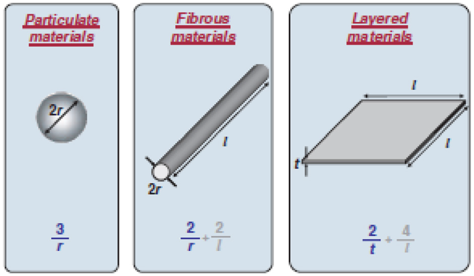
The general idea of nanocomposites is based on the concept of creating a very large interface between the nanosized-building blocks and the polymer matrix. Aggregation phenomenon is a major subject in composites having spherical nanoparticles. ⁷ Figure 1 shows usually used particle geometries and their respective surface-to-volume ratios. For the fibrous and layered material, the surface area/volume is dominated, particularly for nanomaterials, by the primary term within the equation. The secondary term (2/l and 4/l) is very small compared to the first term and can be neglected. Therefore, logically, the surface area-to-volume ratio is affected by a change in particle diameter, layer thickness, or fibrous material diameter from the micrometer to nanometer range by three orders of magnitude.^8,9

Figure 1.

Surface to volume ratio.^8,9

Woven fabrics are made by the interlacing of warp (0°) fibers and weft (90°) fibers in a regular pattern or weave style like plain, twill, and satin. Recently, due to better results, the utilization of 3D woven fabrics as reinforcing elements for structural composites have attained increased interest in the composites community. Traditional composite laminates made of 2D fabrics as reinforcement have low out of plane properties, while 3D fabrics give reinforcement through the thickness direction. This leads to better out of plane properties compared to composites based on 2D fabric and it can increase resistance to delamination.^10,11 Lode Daelemans et al. ¹⁰ used virtual fiber and digital element concept in simulation methodology to observe mechanical behavior of 3D woven fabrics. Numerical simulation of the composite material is important due to the difficulty in simulating actual test conditions with special configurations or observing the occurrence of internal damages at different loading levels. Finite element method is a suitable numerical method to carry out the simulation. This review aims to focus on knowledge in synthesis, fabrication, and material characterization and some recent advances in modeling and simulation techniques for polymer nanocomposites.

Properties of fiber and matrixs

Basalt fiber (BF)

The use of basalt fibers is possible in many areas due to its good properties. It shows excellent resistance to alkalis, similar to glass fiber, at a much lower cost than carbon and aramid fibers. ¹² Basalt is a volcanic mineral, dark or black. Its rocks are heavy, tenacious, and resilient. Compared to glass, its density is about 5% higher. The chemical composition of the basalt depends upon the mineral deposit. It contains oxides by weight percentage: SiO₂ (48.8–51), Al₂O₃ (14–15.6), CaO (10), MgO (6.2–16), FeO + Fe₂O₃ (7.3–13.3), TiO₂ (0.9–1.6), MnO (0.1–0.16), Na₂O + K₂O (1.9–2.2).^12,13 Performance of BF lies in between the performance carbon and glass fiber. Basalt fiber gives excellent tensile strength and greater failure strain than E-glass fibers and carbon fibers respectively; also it provides better corrosion resistance. Essential properties and cost of basalt, carbon and glass fiber are displayed in Table 1.

Table 1.

Essential properties and cost of basalt, carbon and glass fiber. ¹³

Fiber	Density (g/cm3)	Diameter (µm)	Tensile strength (GPa)	Modulus of elasticity (GPa)	Cost (USD/kg)
Basalt	2.8–3.0	9–17	2.6–3.2	93–110	0.34–0.37
Carbon	1.78	8	2.8–5.0	230	16.32
Glass	2.5–2.6	10–15	1.0–2.7	80–90	0.27–0.30

The useful properties of BF are excellent thermal properties, better vibration damping capacity, better tensile strength and electromagnetic properties, high corrosion and radiation resistant, eco-friendly, non-toxic, and easy for handling. ¹⁴

Carbon fiber

Carbon fiber contains not less than 92% carbon by weight fraction, while the fiber which contains at the minimum 99% carbon by weight is known as graphite fiber. The useful properties of carbon fibers are low density, excellent tensile properties, good thermal and electrical properties, excellent resistance to creep, high chemical and thermal stability in absence of oxidizing agent.

They are widely used as a reinforcing element in composites in the form of different woven patterns, prepregs, continuous, and chopped fibers.^15,16 Carbon fibers derived from polyacrylonitrile (PAN) are turbostratic and have high tensile strength.

Glass fiber

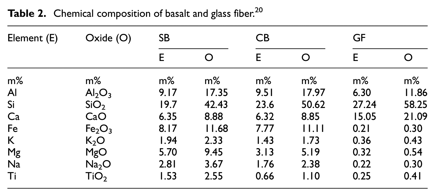
Glass fiber composites are widely used in aerospace and automotive industries due to its properties such as low density, high strength, and easy processing. ¹⁷ Due to better characteristics like strength, resistance to impact, fatigue, and low density, S-2 glass fiber reinforced polymeric composites are used in automobile, aerospace industries for various parts as compared to conventional glass fibers.^18,19 The chemical composition of S glass fiber is 55% SiO₂, 11% Al₂O₃, 6% B₂O₃, 18% CaO, 5% MgO, 5% other. Table 2 shows chemical composition of short basalt (SB), continuous basalt (CB), and glass fiber. ²⁰

Table 2.

Chemical composition of basalt and glass fiber. ²⁰

Element (E)	Oxide (O)	SB		CB		GF
		E	O	E	O	E	O
m%	m%	m%	m%	m%	m%	m%	m%
Al	Al2O3	9.17	17.35	9.51	17.97	6.30	11.86
Si	SiO2	19.7	42.43	23.6	50.62	27.24	58.25
Ca	CaO	6.35	8.88	6.32	8.85	15.05	21.09
Fe	Fe2O3	8.17	11.68	7.77	11.11	0.21	0.30
K	K2O	1.94	2.33	1.43	1.73	0.36	0.43
Mg	MgO	5.70	9.45	3.13	5.19	0.32	0.54
Na	Na2O	2.81	3.67	1.76	2.38	0.22	0.30
Ti	TiO2	1.53	2.55	0.66	1.10	0.25	0.41

Thermoset resin

Thermosetting material cannot be remelted or change its shape while hardened. Three-dimensional molecular chain formed during curing is called cross-linking. Due to cross-linking, the molecules become rigid and cannot be remelted and reshaped. Rigidity and thermal stability depend upon a number of cross-linking. Due to brittleness, some filler materials and reinforcing elements are added in thermosets to enhance properties. In most composite manufacturing techniques like resin transfer molding, pultrusion and wet layup, resin is used in liquid form, it provides better fiber impregnation and easy processability. Thermosetting material provides good dimensional and thermal stability, rigidity and resistance to chemical and solvent. Polyesters, epoxy, phenolics, polyamides, and vinyl esters are commonly used resin materials in thermoset composites.

Epoxy is the most commonly used resin material, which is used in various applications, from sporting goods to aerospace. Epoxy, a liquid resin, contains a number of epoxide groups such as diglycidyl ether of bisphenol A (DGEBA) and bisphenol F (DGEBF). Bisphenol F (DGEBF) is widely used in epoxy resin thermosetting products. In an epoxide group, there is a three-membered ring of two carbon atoms and one oxygen atom. In addition to this starting material, other liquids such as diluents to reduce its viscosity and flexibilizers to increase toughness are mixed. The curing (cross linking) reaction takes place by adding a hardener or curing agent. EPON resin 862 (diglycidyl ether of bisphenol F) offers high wettability, good balance of mechanical, adhesive, and electrical properties and also good chemical resistance, superior physical properties. ²¹ Flexure and interlaminar properties of plain weave woven glass fiber reinforced epoxy composites can be increased by modification of matrix by using Tetraethyl orthosilicate (TEOS) electrospun nanofibers (ENFs) with proper amount in epoxy.^22–24

Manufacturing methods for fibers

Basalt fiber

Basalt fibers are manufactured by centrifugal-blowing, centrifugal-multi-roll, and melt Blowing techniques. In centrifugal blowing, quarried basalt rock is crushed, washed, and loaded into a bin attached to feeders that transfer the material into melting baths in gas-heated furnaces. Processing of BF is much easier than glass fiber due to its simplicity. Crushed basalt is conveyed to the furnace through a feed line and heated to1450°C for melting. Basalt rock melt then delivered to the fiber spinning machine to form basalt fibers as shown in Figure 2.

Figure 2.

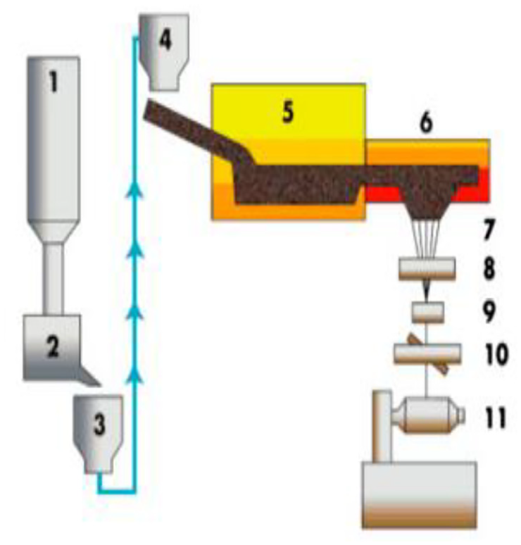
BF spinning. ¹⁴ (1) Raw basalt storage, (2) mixing unit, (3) conveying media, (4) batch charging station, (5) primary melt unit, (6) secondary heat controlled unit, (7) bushings with orifices, (8) size control applicator, (9) strand development, (10) traversing, and (11) winding.

Centrifugal-multi roll system is generally used for the production of fibers for insulation purposes, and consists of a series of rotating wheels. Molten rock is being thrown away as it passes over the first wheel and finally approximate 10 μm diameter fibers are formed with the help of properly aligned wheels. Depending upon applications, similar to traditional glass fibers, continuous fibers are produced by using spinnerjet method. Continuous fibers undergo stretching to achieve precise diameter by controlling speed automatically. A schematic of basalt fiber spinning is shown in Figure 2, in which raw material with appropriate weight and dose is supplied into the furnace through transporting media and it is heated to 1450°C temperature at which melting takes place. Molten basalt is fed to a secondary temperature controlled zone and then it passes through bushing which contains a number of micro holes. The number of holes and their diameter depends on end application. Filaments formed are converted into a single thread of continuous basalt fiber.

Resulting filament diameter depends upon molten material viscosity and orifice size. These strands are silane treated to bestow lubricity and matrix compatibility.^14,25,26

Carbon fiber (CF)

Carbon fiber contains mostly carbon atoms with 5–10 μm in diameter. The raw material used to make carbon fiber is called the precursor. About 90% of the carbon fibers produced are made from polyacrylonitrile (PAN). The remaining 10% is made from rayon or petroleum pitch. Carbon fibers are generally produced from precursor fibers by controlled pyrolysis. Precursor fibers undergo stabilization at around 200°C–400°C by an oxidation process. The stabilized fibers then undergo a carburization process at about 1000°C to remove non carbon elements. Carbonization process is followed by graphitization, in which fibers are subjected to high temperature at about 3000°C to get high carbon content and modulus of elasticity in the direction of fiber. Adhesion of carbon fibers with composite matrix is improved by using post-treatment of inert surfaces.^{15,16,27–29}

Glass fiber

All glass fiber types contain more than 50% silica and other ingredients include the aluminum, calcium and magnesium oxides, and borates. A batch of exact quantities and thoroughly mixed raw materials is formed before being melted into glass. This batch is converted into molten material in a furnace at about 2300°F (1250°C) and then completely molten glass is allowed to flow through bushings having small holes. To achieve better processability of glass strands and to give good adhesion with resin, glass filaments are chemically treated.

Synthesis of nanofiber

Electrospinning

One among the foremost techniques for developing continuous nano-scale fibers with diameters ranging from tens to hundreds of nanometers is electrospinning. ²³ It can produce ultra-thin nanofibers at random, as well as aligned nanofibers, from different polymers, ceramics.

In this method, fibers of varying diameters from solution gelatin (sol-gel) are formed with the help of an electric field created by a high voltage power supply. Figure 3 shows electrospinning set up, in which feed rate of solution droplet is controlled by programmable distributing pump. ¹⁸ One of the dominating properties of electrospun nanofibers is high surface to volume ratio compared to ordinary fibers. It shows higher porosity and small size pores and provides better delamination resistance. Shinde et al. ²⁴ used electrospinning to produce TEOS ENFs with isotropic properties in the form of non-woven mat. ENFs mat, can improve performance and life of structural parts in automotive and aerospace application because of reduced sensitivity against damage progression.

Figure 3.

Electrospinning set up.^30–32

Manufacturing techniques for composites

Increased relative surface area and quantum effects are two important factors, which results in significantly different properties of nanocomposites from other material properties. ²⁸ Some nanocomposites indicate properties predominated by the interfacial interactions and others display the quantum effects associated with nano dimensional structures.^9,33 Wet layup, prepreg processing, resin transfer molding, vacuum assisted resin transfer molding, autoclave method, pultrusion process, filament winding, etc. are broadly utilized techniques for manufacturing conventional composite parts.^9,22,34

Wet lay up

Wet layup is the simplest manufacturing method in which resin is put only in the mold. Resin impregnated fiber is achieved with the help of a roller. Required thickness of composite is achieved by addition of another layer of reinforcing element and resin. Due to its flexibility, it allows various fabric materials to form composites. Due to manual reinforcement, it is also known as hand layup method.^9,22 Presence of voids results in poor mechanical properties such as compressive strength, interlaminar shear strength, and non- uniformity in the final product.^9,35

Pultrusion process

This process is less expensive and used to manufacture composites at high volume rate by pulling fibers which are resin impregnated, through a die. The pultrusion process is not suitable for thin-walled, close tolerance parts and complex shapes. A chance of void formation is another drawback.^9,22 Schematic representation of the pultrusion process is shown in Figure 4.

Figure 4.

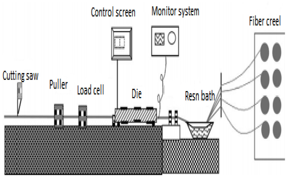
The schematic representation of the pultrusion process. ³⁶

Resin transfer molding (RTM)

In this process, mold cavity is formed based on required shape and preform is kept into the cavity. Matching mold half is mounted on the principal half and they are cinched together. Then resin is allowed to flow under pressure in the mold through various types of ports. The part is then removed from the mold after completion of the curing cycle. Designers and textile manufacturers are using RTM to fabricate parts for key structures due to advances in technology related to resin.^9,28,37 Schematic representation of the RTM process is shown in Figure 5. In view of vacuum impregnation, RTM is inexpensive compared with conventional autoclaving due to savings in materials and labor cost. Health, safety benefits, and reductions in tooling costs compared to positive pressure driven RTM are advantages of RTM. ³⁸

Figure 5.

Schematics of the RTM process. ²²

Vacuum assisted resin transfer molding (VARTM)

VARTM is developed from the RTM process. Figure 6 shows VARTM set up. In this process, one-sided mold is used in which fibers are placed and the top side is vacuum-tight sealed with the help of either rigid or flexible cover. A resin is allowed to flow into the preform through ports by using a vacuum pump. This method is used to achieve high volume fraction of fiber up to 70% and better mechanical properties are obtained in the part.^9,22,39 Resin flow depends on viscosity; high viscosity affects the resin flow. Presence of nanoparticles in the matrix resin affects cure kinetics and make complications in the changed viscosity of resin,^9,40 which results in non-uniform distribution of resin over entire fiber volume.^9,41

Figure 6.

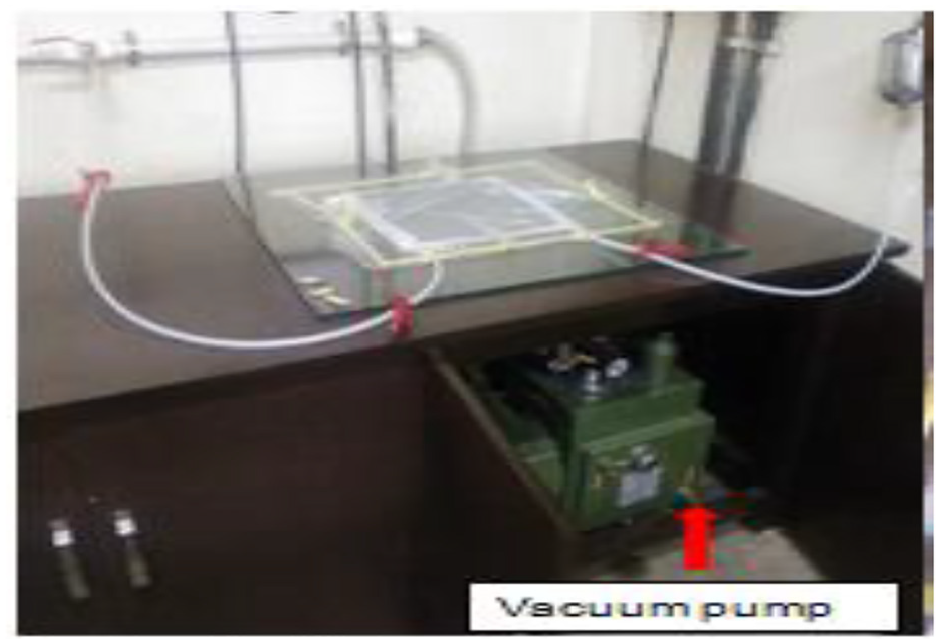
VARTM setup.

Structural Reaction Injection Molding (SRIM)

This process is an adaptation of the reaction injection molding, in which a mixture of resin (resins with different properties) is injected into mold. Due to the absence of reinforced members, components manufactured by this process are feeble. The RIM process produces components at high volume rate. ²²

Filament winding method

In this process, resin impregnated fibers are wound over a revolving shaft at the proper angle. In this process, the carriage unit moves back and forth and the mandrel rotates at a specified speed. By controlling the motion of the carriage unit and the mandrel, the desired fiber angle is generated. The process is very suitable for making tubular parts. ²²

Processing of nanomaterials

One of the regular difficulties in mixing hard (inorganic fillers) and soft (polymers) materials is the dispersion of nanoparticles. Usually, this has a lot to do with the filler surface energy. For instance, the SiO₂ particles were regularly discovered agglomerated in polymer matrices. ³⁹ Mixing assisted with high energy shear force produces better outcomes by making enough energy to the separate agglomeration of particles. Proper dispersion of nanoparticles in the polymer matrix can be achieved by using a high energy sonication process. The force required to separate small nanoparticles depends upon particle to particle interaction and the viscosity of the resin in which they are dispersed.^39,42 The performance of the nanocomposites in strength and modulus may be affected by sonication amplitude. ²¹

Intercalation method

This method follows a top down approach in which fillers downsized to nano dimensions. In this process, delamination of layered silicates takes place by intercalating an organic compound into the interlayer space of silicate, bringing about plate-like nanofillers uniform dispersion.^43–45

In situ polymerization method

This technique utilizes polymerization reaction. In this method, dispersion of inorganic nanoparticles in monomer solution happens and subsequent blend undergoes standard polymerization technique. Polymeric nanocomposites have been synthesized from metal precursors and matrix polymers through the simultaneous formation of metal particles. Proper dispersion of the filler in monomer solution is achieved in In Situ Polymerization technique. Metal precursors wettability with monomer is enhanced by organic modification.^43–45

Sol gel method

This is a bottom up method combined with In Situ formation of nanofillers and In Situ polymerization by using sol gel technique. Dispersion of inorganic fillers with dimension less than the molecular chain length of polymer matrix is possible by this method.^43–45

Direct mixing of polymer and nanofillers

Similar to the intercalation method, this method follows a top down approach in which aggregated fillers are separated during the mixing process. Polymeric composites containing nanofillers or micro-sized fillers are generally manufactured by this method. Polymer and fillers are mixed in two ways. The first is a melt compounding method in which mixing of polymer and nanofillers occurs in the absence of any solvents. The second is a solution-mixing method in which mixing of fillers and polymers occur in a solution.^43–45

Effect of nanomaterials on mechanical properties of composites

Delamination of the composite depends upon the interlaminar shear strength. Use of electrospun TEOS nanofiber in the S-2 glass fiber showed significant improvement in the interlaminar shear strength that will improve the delamination of the composite and could be useful for the structural application. The tensile strength of composite is enhanced by 2.1%, while compressive strength and modulus are decreased by 8.4% and 36.8% respectively due to the brittleness of the electrospun TEOS nanofiber. ¹⁸ Shinde et al. ³⁰ studied mechanical properties such as tensile strength and tensile modulus of neat epoxy resin (Epon 862/W), neat resin with nanofibers mat, and neat resin with 0.08%–0.4% wt. of chopped electrospun TEOS nanofibers. 0.4% wt. chopped nanofibers mixed with the resin, showed about 23% increase in tensile strength compared to the tensile strength of the neat resin. Improved properties are due to strong adhesion between electrospun TEOS nanofibers and resin during the cross linking of polymer in curing and also due to uniform distribution of nanofibers during sonication. Compared to 0.08% wt. of chopped electrospun TEOS nanofibers in resin, 0.4% wt. of chopped electrospun TEOS nanofibers in resin showed strong adhesion, this leads to improving strength and slight improvement in modulus. Significant improvement in the fracture toughness of composite is achieved by the addition of electrospun TEOS nanofibers. ³⁰ Shinde et al. ³¹ studied the performance of nanoengineered beams fabricated by interleaving TEOS ENFs between the laminated fiberglass composites and results were validated by developing a detailed three-dimensional finite element model. It was observed that there is a strong agreement between experimental results and results of the progressive deformation and damage mechanics from the finite element model. Overall, nanoengineered beams showed improvement in the short beam strength and 30% improvement in energy absorption as compared to a fiberglass beam without the presence of nanofibers. Shukla et al. ⁴⁶ studied the effect of carbon nanotube and graphene on the mechanical properties of epoxy based nanocomposites. The results indicated that incorporation of carbon nanotube and graphene simultaneously in the epoxy revealed significant improvement in the mechanical properties compared to the incorporation of a single nanofiller into epoxy, because of formation of strong bonding. Mishra et al. ⁴⁷ developed a novel technique to fabricate composite materials containing TiO₂ nanoparticles, polysiloxane resin, and basalt fabric. They investigated the loading effect of TiO₂ nanoparticles on the thermal and mechanical properties of basalt fabric reinforced polysiloxane composite materials. The result shows that tensile properties of polysiloxane matrix can enhance with the addition of a lower percentage of TiO₂ nanoparticles, which can be attributed to increasing friction force between the nanofillers and the matrix, resulting in increased mechanical interlocking in the composite system. Heat distortion temp (HDT) of the nanocomposite increases with the increase in nanoparticle content of the polymer. ⁴⁷ Erkliğ et al. ⁴⁸ investigated the effect of inclusion of nanographene on mechanical behavior of glass/basalt reinforced hybrid polymer composite. The results have shown that the incorporation of nanographene results in an enhancement of the mechanical properties. Khandelwal et al. ⁴⁹ summarized recent development in basalt fiber reinforced epoxy polymer composite. They discussed the drawbacks that occurred due to weak fiber matrix interface and suggested strategies for improving fiber matrix interaction through the modification of fiber surface and multiscale reinforcement. The laminated fiber reinforced composites are used increasingly for structural applications in the automotive, energy, and aerospace sectors due to its lightweight, easy manufacturing technique, and better performance under loading at high temperature. Shinde et al. ³² investigated the effect of TEOS ENFs on short beam strength and damage mechanism of laminated fiberglass composite using an optimized weight of non-woven TEOS ENFs sheet between plies of the laminate. For better wetting purposes an additional epoxy resin film was used to ensure better soaking and impregnation of nanofibers. The result showed that short beam strength of nanoengineered composites improved by 16% with the addition of TEOS ENFs and also the strain energy absorbed before complete failure of nanoengineered composites improved by 30%, 7%, 20%, and 4% for various stacking sequences. The study also indicates that the nanoengineered composite will be suitable for numerous applications ranging from automobiles, helmets, and applications involving blast resistance material. ³² Fu et al. ⁵⁰ presented a recent review on synthesis, characterization, and mechanical behavior of polymer nanocomposite. They studied the effect of interfacial strength on mechanical properties of polymeric nanocomposite. Mankodi ⁵¹ observed improvement in mechanical properties of basalt fiber reinforced composite with the increase in the fibers reinforcement content in the matrix material. In that study, improvement in mechanical properties of the laminate was observed with increase in the content of basalt filler. Hence as the content of basalt filler increases in the laminate, it will increase the mechanical properties of the laminate. Due to better properties and proper atomic arrangement of CNT_S, mechanical, electrical and thermal properties of polymeric composites can be improved by using CNTs. CNTs, because of their small size, can be embedded in soft and light materials to improve mechanical properties. At the functionalization level, nanotubes do not have a significant difference in tensile strength. Nano mechanical interlocking was observed at interface between nanotube and polymer. Increased friction between filler and matrix material due to difference in thermal expansion, increases pullout strength of nanotubes. ⁵² Kumar et al. ⁵³ analyzed a number of research papers related to hybrid nanocomposites and studied the effect of graphene with other nanofiller on the mechanical properties of composites. They observed that the inclusion of graphene filler results in enhancement in the mechanical properties of graphene composites.

Characterization techniques for hybrid nanocomposites

Homogeneity of the mixture of reinforcing element and matrix plays a significant role in the success of chemical synthesis of ceramic nanoparticles. Porous media are usually described by various simple measures; mainly recognized measures are porosity, size of pore, surface area, and complexity in distribution of porous size. Experimental data is fitted to one of the suitable models in order to acquire values of mentioned measures. Various techniques for characterization have been utilized broadly in polymeric nanocomposite research.^9,54–56 X-ray diffraction, small angle X-ray scattering, wide angle X-ray diffraction, scanning electron microscopy and transmission electron microscopy, atomic force microscope are widely used characterization techniques.

Scanning electron microscopy (SEM)

Most widely used technique to observe surface morphology is scanning electron microscopy. Vacuum assisted electron beam is collimated by lenses, centered by lens, and scanned with the help of electromagnetic coil across the sample surface. In the Scanning Electron Microscope, an electron gun is used to probe the test sample. Cathode emitted electrons are accelerated through the electrical field by passage and centered to the optical image of source. Performance of scanning electron microscope depends upon the current, size and shape of source, electron beam speed.^9,54–59 As an example, Figure 7 shows an SEM image of tetra ethyl orthosilicate (TEOS) electrospun nanofiber after sintering.

Figure 7.

SEM image of electrospun nanofiber. ²⁴

Scanning tunneling microscopy (STM)

Scanning Tunneling Microscopy yields a true three-dimensional topography of surfaces on an atomic scale. It provides a better result than scanning electron microscopy, with the possibility of extending it to work function profiles (fourth dimension). It is a nondestructive technique (energy of the tunnel “beam” 1 meV up to 4 eV) and uses fields down to three orders of magnitude less than field-ionization microscopy. In STM, for electrons to tunnel across the gap, approximately 0.5 nm distance is kept between surface and tip.^60,61 Schematic of the STM process is shown in Figure 8.

Figure 8.

Schematic of STM. ⁶²

Atomic force microscopy (AFM)

Atomic force microscopy or AFM is used to observe a three-dimensional surface at the nanometer scale. AFM is also called scanning force microscope (SFM). Flexible cantilever is scanned comparative to a surface in atomic force microscope (AFM). Flexible cantilever has a sharp tip from its free end in the direction of the surface under test. Deflection of cantilever tip depends upon forces between the tip of cantilever and test surface and deflection of cantilever is monitored to measure surface topography. Vander Waal’s, magnetic, electrostatic, and viscous forces are generated between the cantilever tip and sample surface. There are two operating modes of the cantilever. In the first mode, a tip is in contact with the sample surface and in the second mode; approximately 5–500 A distance is maintained between tip and sample surface. ⁶³ Figure 9 shows the schematic of AFM.

Figure 9.

Schematic of AFM. ⁶²

Transmission electron microscopy (TEM)

Transmission Electron Microscopy gives surface morphology along with the size and shape of particles. By this technique, a beam of photographic film or electrons is generated by a process known as thermionic discharge in the same manner as the cathode in a cathode ray tube or by field emission; they are then accelerated by an electric field and focused by electrical and magnetic fields onto the sample. Another type of TEM is the Scanning Transmission-Electron Microscope (STEM), where the beam can be rastered across the sample to form the image.^55,64

X-ray powder diffraction (XRD)

The unknown crystalline material is identified and characterized by X-ray powder diffraction (XRD). Randomly oriented grains in powder are analyzed efficiently by this analytical technique to ensure all directions are “sampled” by the beam. The point at which Bragg conditions are acquired for constructive interference, a “reflection” is created and relative peak height is commonly corresponding to grain quantity in the favored direction. This technique produces X-ray spectra which give a structural fingerprint of an unknown sample. With this technique it is possible to analyze mixtures of crystalline materials and data of relative peak height can be used to get semi quantitative evaluation of abundances.^9,55,57,65

Small-angle X-ray scattering (SAXS)

Small-angle X-ray scattering (SAXS) is used to quantify nanoscale density differences in a sample. This technique can be used to determine nanoparticle size distributions, resolve the size and shape of macromolecules, determine pore sizes, characteristic distances of partially ordered materials, and much more. This is achieved by analyzing the elastic scattering behavior of X-rays when traveling through the material, recording their scattering at small angles (typically 0.1°–10°, hence the “Small-angle” in its name).

Mechanical characterization of FRP composites

Experimental testing of the composites for mechanical characterization of hybrid composites

Short beam strength

Interlaminar failure resistance of fiber reinforced polymer composite is usually characterized by short beam shear test. In this test, beam is loaded under three point bending. Figure 10 shows short beam test set up.

Figure 10.

Short beam test set up.

As stress concentrations are less severe, short-beam shear test has simpler experimental requirements as compared to tensile test. Ease of sample preparation is another advantage of this test, as cross section of specimen can be rectangular. This test method is limited to the use of a span to-thickness ratio of 4 and minimum sample thickness of 2 mm. Short beam strength at the specimen mid plane is calculated by ASTM ⁶⁶

$$\mathrm{F}=0.75\mathrm{x}\frac{P}{b*h}$$

(1)

Where, F = short beam shear strength, MPa

P = maximum load, N

b = specimen width, mm

h = specimen thickness, mm

Flexural strength

The flexural test has become a widely used method for characterizing the flexural properties such as stiffness, strength, and load deflection behavior of fiber-reinforced composites. This test method involves loading a beam under three-point bending. Figure 11 presents flexural test set up.

Figure 11.

Flexure test set up.

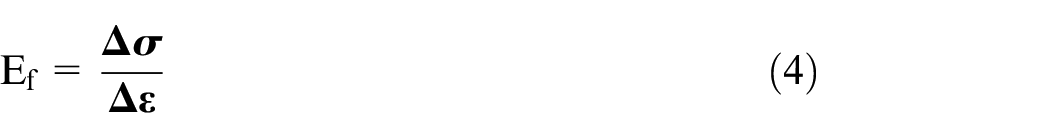
In accordance with ASTM D 7264 standard, ⁶⁷ span-to-thickness ratio of specimen is 32:1 and standard specimen width and thickness are 13, 4 mm respectively. To calculate flexural strength, failure occurred on the either one of its outer surfaces, preceding interlaminar shear failure or crushing failure under a support or loading nose is considered. Flexural properties are calculated by,

$${\sigma }_{\mathrm{f}}=\frac{3\mathbf{FL}}{2\mathbf{b}{\mathbf{h}}^2}$$

(2)

Where,

σ_f = flexural stress at outer surface at mid span, MPa

F = applied force, N

L = support span, mm

b = width of test specimen, mm

h = thickness of test specimen, mm

$${\mathrm{\epsilon }}_{\mathrm{f}}=\frac{6\mathbf{\delta }\mathbf{h}}{{\mathbf{L}}^2}$$

(3)

Where,

ε_f = maximum strain at outer surface, %

δ = mid span deflection, mm

L = support span, mm

H = thickness of test specimen, mm

$${\mathrm{E}}_{\mathrm{f}}=\frac{\mathit{\Delta }\mathbf{\sigma }}{\mathit{\Delta }\mathbf{\epsilon }}$$

(4)

Where,

E _f = flexural modulus of elasticity, MPa

$\mathit{\Delta }\mathbf{\sigma }$  = Difference in flexural stress between the two selected strain points, MPa

$\mathit{\Delta }\mathbf{\epsilon }$  = difference in average strain between the two selected strain points

Tensile test

Tensile test determines in-plane tensile properties such as tensile strength, tensile modulus of elasticity, poison’s ratio of high modulus fiber reinforced polymer composites. Figure 12 shows tensile test set up.

Figure 12.

Tensile test set up.

In accordance to ASTM D 3039 standard, ⁶⁸ most common specimen is a constant rectangular cross section, 250 mm long and 25 mm wide. A strain gauge or extensometer is used to determine tensile modulus. Typical test speed for standard test specimen is 2 mm/min. Tensile properties are calculated by using following equations.

$${\sigma }_t=\frac{P}{w*t}$$

(5)

Where,

${\sigma }_{\mathrm{t}}$  = tensile stress, MPa.

P = maximum load, N

W = specimen width, mm

t = specimen thickness, mm

$${\mathrm{E}}_{\mathrm{t}}=\frac{\mathit{\Delta }\mathbf{\sigma }}{\mathit{\Delta }\mathbf{\epsilon }}$$

(6)

Where,

E _t = tensile modulus of elasticity, MPa

$\mathit{\Delta }\mathbf{\sigma }$  = difference in compressive stress between the two selected strain points, MPa

$\mathit{\Delta }\mathbf{\epsilon }$  = difference in average tensile strain between the two selected strain points

Compression test

Compression test determines in-plane compressive properties such as compressive strength, compressive modulus of elasticity of high modulus fiber reinforced polymer composites. Figure 13 shows compression test set up.

Figure 13.

Compression test set up.

The most common specimen is a constant rectangular cross section, 140–155 mm long and 25 mm wide as per ASTM D 3410 standard. ⁶⁹ Compressive stress is calculated by,

$${\sigma }_c=\frac{P}{w*t}$$

(7)

Where,

${\mathrm{\sigma }}_{\mathrm{c}}$  = compressive stress, MPa

P = maximum load, N

w = specimen width, mm

t = specimen thickness, mm

$${\mathrm{E}}_{\mathrm{c}}=\frac{\mathit{\Delta }\mathbf{\sigma }}{\mathit{\Delta }\mathbf{\epsilon }}$$

(8)

Where,

E _c = compressive modulus of elasticity, MPa

$\mathit{\Delta }\mathbf{\sigma }$  = difference in compressive stress between the two selected strain points, MPa

$\mathit{\Delta }\mathbf{\epsilon }$  = difference in average compressive strain between the two selected strain points

Multi scale modeling and simulation techniques

The characteristics of material were identified through observation via experiments. The development of a model, which foresees the observed behavior, is based on proper measurement of observed data. Figure 14 shows a schematic of the developing theory process. Development of theory is based on a model, which is further used for comparison of predicted experimental properties through simulation. Comparison used for validation of theory or for improvement of theory based on modeling data through a feedback loop. Therefore, accurate modeling and simulation techniques play an important role in improvement of a realistic theory of depicting the structural properties of materials.

Figure 14.

Schematic of developing theory process.

Figure 15 shows different material modeling techniques. Finite element method and boundary element method are some computational micromechanics incorporate techniques. Eshelby method, Halpin Tsai approach are some specific micromechanics techniques. Molecular mechanics, molecular dynamics, Ab Initio, and Monte Carlo technique are some modeling tools.

Figure 15.

Diagram of material modeling techniques. ⁷⁰

Figure 16 shows a wide range of length and time scales for specific modeling methods. Computational chemistry techniques used to predict atomic structure are applicable for the smallest length and time scales. Computational mechanics is utilized to predict structure and properties of materials, for macroscopic length and time scale. Computational chemistry and mechanics modeling techniques are based totally on well-established engineering and science principles. However, due to lack of general modeling techniques on intermediate time and length scales compared to well-developed modeling methods on small and large length and time scale, multi-scale modeling methods are used to predict structural and mechanical properties through bridging scales. ⁷³

Figure 16

Length and time scales for determination of polymeric nanocomposite properties. ⁷³

Analytical models for composites

Halpin Tsai model

Halpin Tsai model provides hypothetical analysis to predict Young’s modulus, shear modulus, and bulk modulus, of unidirectional composites as a function of fiber volume fraction and aspect ratio of filler. This method can be applicable for different reinforcement filler geometries such as flake like or fiber like fillers. The modulus of elasticity of composite material in Halpin Tsai model is given as^70,71

$$\frac{{\mathrm{E}}_{\mathrm{f}}}{{\mathrm{E}}_{\mathrm{m}}}=\frac{1+{\zeta }_{\eta }{\varphi }_f}{1-\eta {\varphi }_f}$$

(9)

$$\eta =\frac{\frac{{\mathrm{E}}_{\mathrm{f}}}{{\mathrm{E}}_{\mathrm{m}}}-1}{\frac{{\mathrm{E}}_{\mathrm{f}}}{{\mathrm{E}}_{\mathrm{m}}}+\zeta }$$

(10)

Where E_f, E_m, and E_c are modulus of elasticity of filler material, matrix, and composites, respectively, ϕ _f is volume fraction of filler material, while parameter f depends upon geometry of filler and direction of loading. $\zeta$  = 2 $\frac{l}{d}$ for fibers or 2 $\frac{l}{t}$ for disk like platelets. l, t, and d are the length, thickness, and diameter of dispersed filler materials, respectively.

Hui Shia model

Hui Shia model is employed to predict the elastic moduli of composites with unidirectional aligned platelets for the simple assumption of perfect interfacial bonding between the polymer matrix and platelet fillers, which is given by^70,72

$$\frac{{\mathrm{E}}_{\mathrm{c}}}{{\mathrm{E}}_{\mathrm{m}}}=\frac{1}{1-\frac{{\mathrm{\Phi }}_{\mathrm{f}}}{4}[\frac{1}{\mathrm{\xi }}+\frac{3}{\mathrm{\xi }+\mathrm{A}}]}$$

(11)

$$\mathbf{\xi }={\mathrm{\Phi }}_{\mathrm{f}}+\frac{{\mathrm{E}}_{\mathrm{m}}}{{\mathrm{E}}_{\mathrm{f}}-{\mathrm{E}}_{\mathrm{m}}}+3(1-{\mathrm{\Phi }}_{\mathrm{f}})\left[\frac{(1-g){\alpha }^2-\frac{g}{2}}{{\alpha }^2-1}\right],$$

(12)

$$\mathbf{g}=\frac{\pi }{2}\alpha ,$$

(13)

$$\mathbf{A}=(1-{\mathrm{\Phi }}_{\mathrm{f}})\left[\frac{(3({\mathit{\alpha }}^2+0.25\mathit{g})-2\mathit{\alpha }2)}{{\mathit{\alpha }}^2-1}\right],$$

(14)

Where α is the inverse aspect ratio of dispersed fillers and α = t/l for disk-like platelets.

Modified rule of mixture (MROM)

Conventionally, the composite modulus E_c can also be estimated by using a modified rule of mixture (MROM) with flake-like fillers shown as ⁷²

$${\mathrm{E}}_{\mathrm{c}}={\mathrm{\Phi }}_{\mathrm{f}}{\mathrm{E}}_{\mathrm{f}}\left(\mathrm{MRF}\right)+(1-{\mathrm{\Phi }}_{\mathrm{f}}){\mathrm{E}}_{\mathrm{m}},$$

(15)

$$\mathrm{MRF}=1-\frac{\ln (\mathrm{U}+1)}{\mathrm{U}},$$

(16)

$$\mathrm{U}=\mathrm{1}-\sqrt{\left(\frac{{\Phi }_{\mathrm{f}}\mathrm{G}}{{\mathrm{E}}_{\mathrm{f}}(1-{\Phi }_{\mathrm{f}})}\right)}$$

(17)

Where, G is the shear modulus of the polymer matrix.

Molecular scale methods

At molecular level, modeling method and simulation technique uses molecules, atoms and their clusters as basic units. Molecular dynamics, molecular mechanics, and Monte Carlo simulation are the most popular methods. At molecular scale, modeling of polymeric nanocomposite is mainly directed toward mechanics of formation, molecular structure, and interactions.

Molecular dynamics (MD)

Molecular dynamics simulation mainly consists of set of initial conditions of particles; representation of forces among all particles and time evolution of the system by finding classical Newtonian equations for all particles within the system. It is a computer simulation technique used to predict relevant physical properties.^73–75 It generates information such as initial atomic position, velocities, and forces to derive macroscopic properties.

Monte Carlo (MC)

MC technique, also called Metropolis method, in which sample population is generated using random numbers. Steps involved in MC simulation are: (i) Conversion of physical problems under investigation into statistical or probabilistic model. (ii) Solving a probabilistic model by numerical sampling methods. (iii) Analysis of acquired data with the help of statistical methods. This technique gives only equilibrium properties, while MD gives non equilibrium properties along with equilibrium properties. ⁷³

Micro scale methods

Micro scale modeling technique aims to bridge the gap between molecular methods and macro scale, meso scale methods, and avoid their weaknesses. Especially, in nanoparticle polymer systems, the study of structural evolution includes the description of hydrodynamic behavior, which is relatively less expensive and easy to handle by continuum methods compared to atomistic methods, and the interactions between nanoparticle and polymer. In contrast, the interactions between components can be examined at an atomistic level but are usually not straightforward to incorporate at the continuum level.

Brownian dynamics (BD)

The process of BD simulation is similar to MD simulations. In BD, an implicit continuum solvent description is used. It presents a new approximation which enables us to perform simulations at micro second timescale. This approach is especially applicable to systems with large time scale gaps governing components motion because it allows much larger time steps by ignoring internal motions of molecules, as compared to MD. ⁷³

Dissipative particle dynamics (DPD)

DPD can be used for simulation of Newtonian and non-Newtonian fluids, on macroscopic time and length scales. Similar to BD and MD, DPD is a particle based technique. Basic unit of DPD is molecular assembly. However, in DPD, particles are defined by their position, momentum, and mass. Sum of dissipative, conservative, and random forces can describe interaction force between two particles of DPD. ⁷³

Lattice Boltzmann (LB)

Lattice Boltzmann is one of the suitable techniques for the effective treatment of polymer solution dynamics. Recently, it has been used to evaluate binary fluid phase separation in the presence of solid particles. This method is started from lattice gas automation which is formed as simplified molecular dynamics with discrete time, space, and particle velocities. Lattice gas automaton comprises of a regular lattice with particles residing on the nodes ⁷³

Time-dependent Ginzburg–Landau method (TDGGL)

This technique is used for simulation of structural evolution of phase separation in polymers and block copolymers. In this method, temperature reduction from the miscible to immiscible region of the phase diagram is simulated by minimizing free energy function. Glotzer has applied this method to polymer blends and particle filled polymer systems. ⁷³

Dynamic DFT method

Dynamic DFT method has been implemented in the software package Mesodyn™ from Accelrys and models polymers dynamic behavior by combining TDGL model with statistics of Gaussian mean field for time advancement of parameters. ⁷³

Mesoscale and macroscale methods

In spite of the importance of understanding the material properties, and molecular structure, their behavior can be made uniform at different scales with respect to different aspects. Macroscopic behavior is generally explained without taking into account discrete atomic and molecular structure and also it is based on assumption of continuous distribution of material throughout its volume, results in average density and can be subjected to surface forces and gravity. Macroscale or continuum methods follow the fundamental laws of (i) continuity, based on conservation of mass; (ii) equilibrium, based on momentum considerations and Newton’s second law; (iii) the moment of momentum principle; (iv) conservation of energy, derived from first law of thermodynamics; and (v) conservation of entropy, derived from second law of thermodynamics. Continuum models based on these laws should be combined with appropriate constitutive equations.

Micro mechanics techniques are utilized to depict the continuum quantities related to extremely small material elements in terms of structure and behavior of the micro constituents due to non-consistency in continuum mechanics at micro level. Thus, local continuum properties are represented statistically by developing representative volume elements (RVE) in micromechanics models. The RVE is formed to check consistency of length scale with the smallest constituent that has a first order effect on the macroscopic behavior and is further used in full scale model. The micromechanics technique can represent interfaces between discontinuities, constituents, and combined mechanical and non-mechanical properties.

Finite element modeling

Finite element method is a powerful numerical analysis tool used to observe mechanical behavior of composite material that was started in the 1970 decade and then numbers of models are developed to analyze different composites. ⁷⁶ Carbon nanotubes (CNTs), which provide excellent strength and stiffness along with better thermal and electrical properties, were discovered by Sumio Iijima, a Japanese scientist in 1991.^77,78 CNTs were utilized as reinforcing elements to develop nanocomposites. Recently, there has been explosively experimental and analytical work carried out along with finite element modeling on analyzing, developing, and characterizing CNT reinforced polymeric nanocomposites and other nanocomposites. Finite element modeling approaches are multi scale RVE, object oriented, and unit cell modeling.

Multiscale RVE modeling

Li and Chou ⁷⁹ extended the RVE concept at nanoscale and assessed the essential mechanical properties of CNT reinforced polymer composites with the help of 3D nanoscale RVE depending upon finite element and elasticity theory. In RVE, a nanofiller (e.g. carbon nanotube) is surrounded by a matrix and suitable boundary conditions are applied to represent the effects of matrix material. In multi-scale modeling technique, to observe the compressive strength of nano polymer composites, a nanotube is modeled at the atomistic scale and analyzed for matrix deformation using the continuum finite element method. Truss rods were used to simulate the van der Waals interactions between carbon atoms and the finite element nodes of the matrix. Zhang related atomistic simulation with continuum analysis by combining inter atomic potential and CNTs atomic structures into constitutive laws. Feng and Shi ⁸⁰ studied mechanical performance of CNTs surrounded by matrix material in composites by exhibiting a combined atomistic and continuum mechanics technique. Representative volume cells are obtained by modified Morse potential and progressive fracture model.

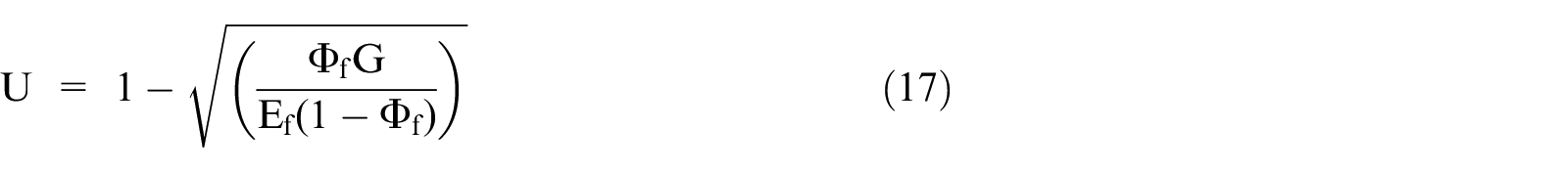
Multiscale RVE incorporates continuum and nanomechanics to bridge the gap between length scales from the nanoscale through mesoscale. Bagha et al. ⁸¹ used square representative volume (RVE) cells in finite element analysis to predict mechanical properties of vapor grown carbon fiber (VGCF) reinforced nanocomposites and compared results with conventional rule of mixtures. They considered two types of arrangement inside the RVE, mainly VGCE inside the RVE and VGCF through RVE. Tserpes ⁸² presented a multi scale RVE to observe the tensile properties of CNT polymeric composites in which rectangular representative cell, whose total volume is filled by the matrix material, is modeled by 3D solid elements, while a nanotube is modeled by 3D beam element. Sanei et al. ⁸³ generated computer simulated microstructures at different length scales to observe change in elastic properties and their results were used to determine RVE size for multiscale analysis. They concluded that RVE is mainly dependent on material properties and microstructure type. Figure 17 shows the synthesis of the RVE. The RVE is synthesized in two steps. (i) Progressive fracture model ⁸⁴ is used to simulate the behavior of the isolated nanotube. The model concept is based on the assumption that CNTs act like space frame structure under loading. Member joints are represented by carbon atoms and a bond between carbon atoms represents load carrying members. Modified Morse potential is used to model the non-linear behavior of carbon-carbon bond and FEM is used to model CNTs structure. (ii) RVE is formed by inserting nanotubes into the matrix. Matrix material and nanotubes are modeled by solid and 3D elastic beam elements respectively.

Figure 17.

RVE synthesis. ⁸⁵

The representative RVE of the composite systems generated for FEA are shown in Figure 18. The flow chart in Figure 19 presents the process of RVE generation for FEA.

Figure 18.

RVEs generated for FEA reinforced with CNT. ⁸⁶

Figure 19.

Steps used to generate RVE for FEA. ⁸⁶

Unit cell modeling

Ordinary unit cell modeling is similar to multiscale RVE modeling. Unit cell is considered as a special RVE of relatively large and definite size and contains sufficient filler count. It is difficult to form analytical models for such a defined unit cell due to its complexity, and numerical technique and simulation become essential. Finite element method is a widely used method to analyze the mechanical behavior of nanocomposite with unit cell. ⁸⁵

Object oriented modeling

Multi scale RVE and unit cell modeling are based on assumptions. These assumptions are, nanofillers can be considered as cylinders, spheres, cubes, or ellipsoids and a number of unit cells or RVEs can be assembled to reproduce nanocomposites. Assumption holds good for simple and homogeneous nanocomposites. The object-oriented modeling is used to overcome the drawbacks of multiscale RVE modeling and unit cell modeling. For example, for irregular filler geometry it’s difficult to capture size, morphology, and reinforcement displacement. In such cases, a relatively new approach, which can capture nanocomposites’ actual microstructure morphology, becomes essential to predict properties and it is object-oriented modeling. It incorporates micrographs into finite element grids. Mesh reproduces original microstructure. ⁸⁵ Chou et al. ⁷⁹ evaluated the mechanical behavior of SiC particle-reinforced Al composites by using 3D object-oriented finite element modeling. Results of modulus of elasticity based on object-oriented models showed good agreement with the experimental and numerical results based on simplified models like prisms, spheres, and ellipsoids.

Figure 20 shows some sample results. As compared to simple analytical models, 3D microstructure-based models can predict properties of particle reinforced composite properties more accurately, as analytical models do not consider micro structural factors which affect mechanical performance of material.

Figure 20.

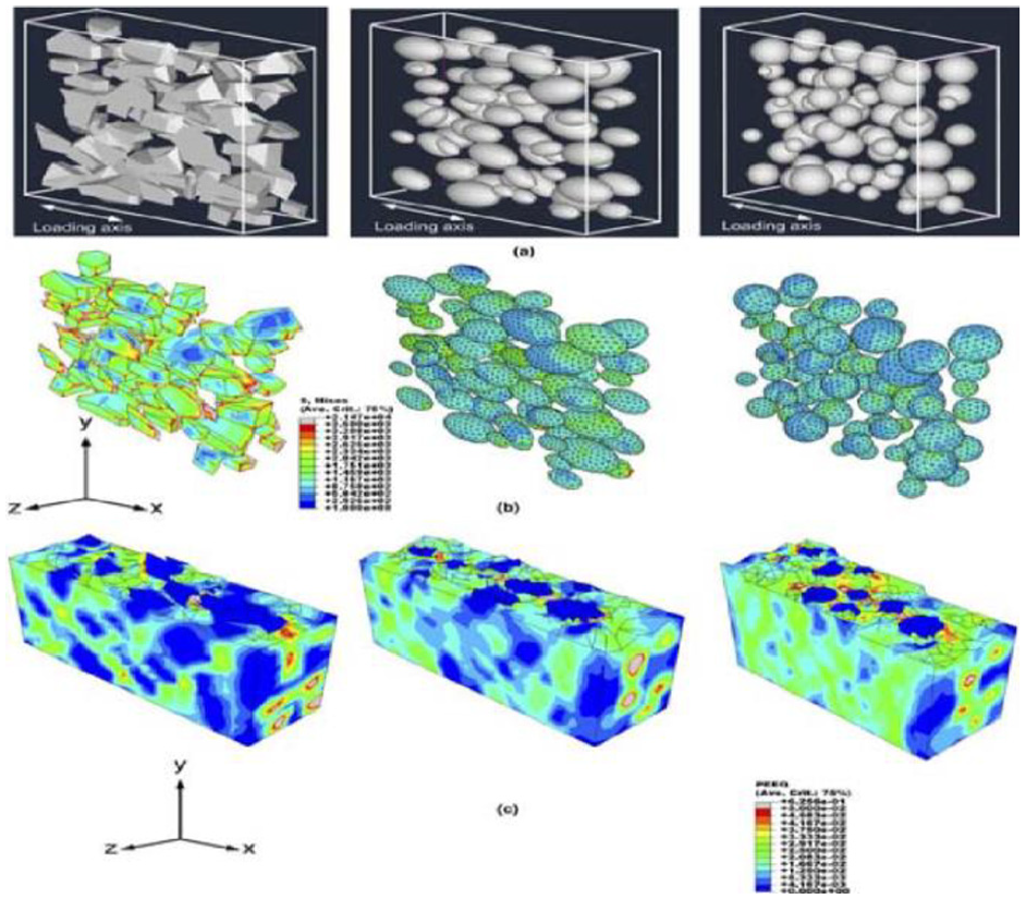
(a) Finite element models containing actual and approximated spherical particles, (b) distribution of von mises stress, and (c) strain. ⁸⁷

Overview of the finite element method

Finite Element method (FEM) which provides an approximate solution to initial and boundary value problems is a general numerical method.

In FEM, spatial discontinuities of non-homogeneous materials are captured by generating preprocessed mesh. FEM also permits complex and nonlinear tensile relationships to be included in the analysis. It has been universally used in geological, biological, and mechanical systems. In FEM, the continuum domain is discretized into subdomains without gaps and overlaps. The sub domains are interconnected at nodes. Figure 21 shows the important steps required for implementation of FEM.

Figure 21.

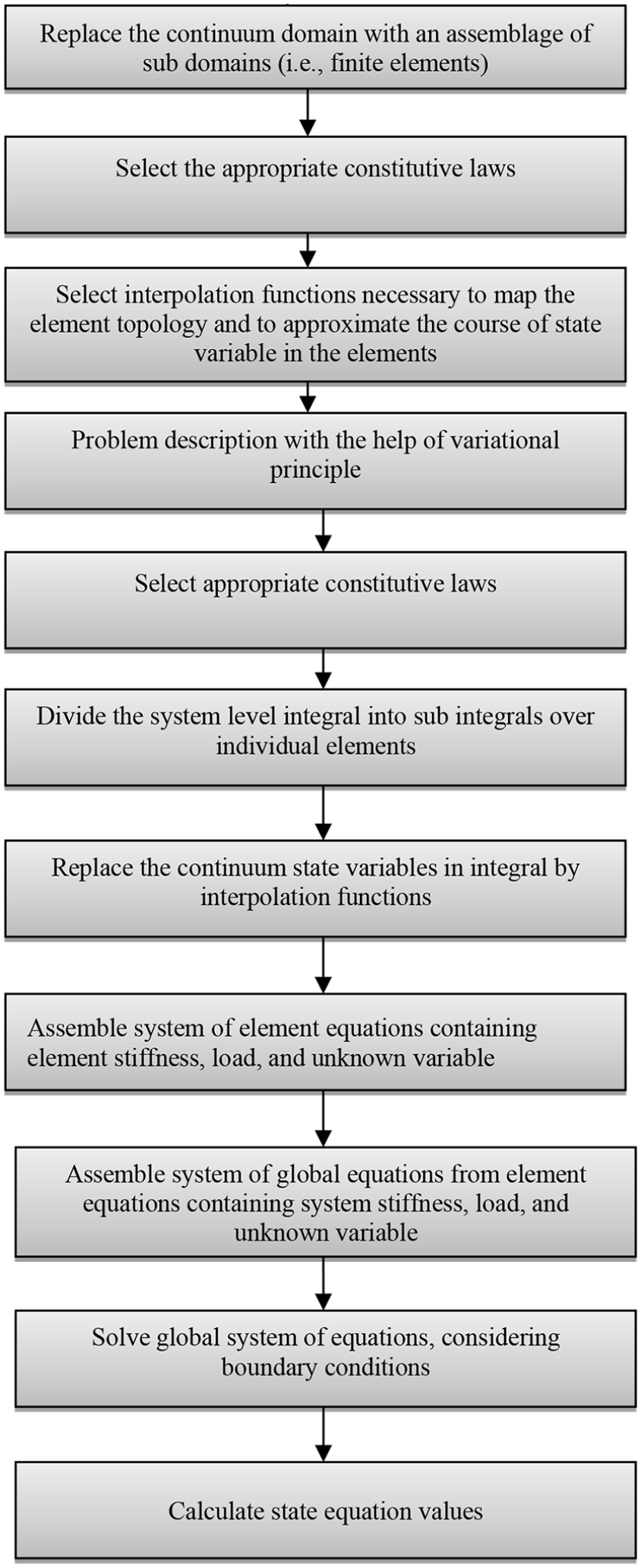
Important finite element method steps. ⁷³

The Finite Element method is formulated using a variational method which requires a functional, which is an integral expression implicitly containing the governing differential equation, to exist for the problem being solved. Governing differential equations with integral expression are often considered as the weak form of differential equations, while the governing differential equations with the boundary conditions are referred to as the strong form. True conditions at every point are required for the strong form, while the weak form only requires that these conditions are satisfied in a normal sense. ⁸⁸ The Finite Element method is based on an approximate version of the weak form of the governing differential equation plus boundary conditions. Energy approach for elastic problems to derive the finite element governing equations is described below.^88,89 Fasanella et al. ⁹⁰ presented Governing differential equations by applying stationary potential energy to the functional for potential energy, Π_P. As per principle of stationary potential energy, at equilibrium, the potential energy is minimized dΠ_P = 0

The total potential energy is a combination of the strain energy from the elastically deformed body, U, and energy of the applied loads, Ω. ⁹⁰

$${\mathrm{\Pi }}_{\mathrm{P}}=\mathrm{U}+\mathrm{\Omega }$$

(18)

The total strain energy for an elastic body is calculated by integrating the strain energy density, ⁹⁰

$$\mathrm{U}=\frac{1}{2}{\int }^{}{\left\{\sigma \right\}}^{\mathrm{T}}\left\{ϵ\right\}\mathrm{dV}=\frac{1}{2}{\int }^{}{\left\{ϵ\right\}}^{\mathrm{T}}\left\{E\right\}\left\{ϵ\right\}\mathrm{dV},$$

(19)

Where $\left\{ϵ\right\}$  = {?_x, ?_y, ?_z, $\gamma$ _xy, $\gamma$ _zy, $\gamma$ _xz} is strain array

The applied load or work potential is given by Fasanella, ⁹⁰

$${\mathrm{\Omega }=-\int }^{}\left\{u\right\}{}^{\mathrm{T}}\left\{F\right\}\mathrm{dV}-{\int }^{}\left\{u\right\}{}^{\mathrm{T}}\left\{T\right\}\mathrm{dS},+{\sum }^{}{\mathrm{ui}}^{\mathrm{T}}\left\{Pi\right\}$$

(20)

Where {u} is the displacement vector, {F} represents the body forces, and the term containing it is integrated over the volume. {T} represents the surface traction, and is integrated over the surface the traction is applied. The last term, {ui}^T·{Pi} is due to point loads applied at point i, and so {u_i} is the displacement at that point.

The global potential energy is then a summation of energies of all the elements, e. ⁹⁰

$$\begin{array}{l}{\mathrm{\Pi }}_{\mathrm{P}}=\sum _e\frac{1}{2}{\int }^{}{\left\{ϵ\right\}}^{\mathrm{T}}\left\{E\right\}\left\{ϵ\right\}\mathrm{dV}-{\sum }^{}{\int }^{}{\left\{u\right\}}^{\mathrm{T}}\left\{f\right\}\mathrm{dV}\\ -{\sum }^{}{\int }^{}{\left\{u\right\}}^{\mathrm{T}}\left\{T\right\}d\mathrm{A}+\sum {\left\{{\mathrm{d}}_i\right\}}^{\mathrm{T}}\left\{{\mathrm{p}}_i\right\},\end{array}$$

(21)

${\mathrm{\Pi }}_{\mathrm{p}}$  =  ${\mathrm{\Pi }}_{\mathrm{p}}$ ( ${\mathrm{D}}_1$ , ${\mathrm{D}}_2$ , …, ${\mathrm{D}}_{\mathrm{n}}$ ). Applying the principle of stationary potential energy yields, ⁹⁰

$$d{\mathrm{\Pi }}_{\mathrm{p}}=\frac{\partial {\mathrm{\Pi }}_{\mathrm{p}}}{\partial {\mathrm{D}}_1}d{\mathrm{D}}_1+\frac{\partial {\mathrm{\Pi }}_{\mathrm{p}}}{\partial {\mathrm{D}}_2}d{\mathrm{D}}_2+...+\frac{\partial {\mathrm{\Pi }}_{\mathrm{p}}}{\partial {\mathrm{D}}_{\mathrm{n}}}d{\mathrm{D}}_{\mathrm{n}}=0$$

(22)

For any zero or nonzero value of $d{\mathrm{D}}_1$ , $d{\mathrm{D}}_2$ , $d{\mathrm{D}}_{\mathrm{n}}$ , then $d{\mathrm{D}}_1$  = 0 for the principle of stationary energy to hold, and so it is required that all $\frac{\partial {\mathrm{\Pi }}_{\mathrm{p}}}{\partial {\mathrm{D}}_{\mathrm{n}}}$ must go to zero, and so for i = 1, 2, …, n.

$$\frac{\partial {\mathrm{\Pi }}_{\mathrm{p}}}{\partial {\mathrm{D}}_{\mathrm{i}}}=0$$

(23)

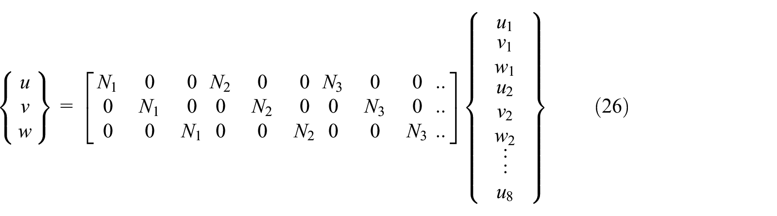
In the Finite Element method, above is solved for the various degrees of freedom, which are determined by the type of finite element chosen. Hexahedron elements, or “brick” elements are used in this formulation. These elements contain three degrees of freedom for every node: x-displacement (u), y-displacement (v), and z-displacement (w). The origin of the element is in the bottom left corner, giving u, v, and w a range of 0–1. With the given coordinates, the eight shape functions obtained for the hexahedron element are

$$\begin{array}{c}{\mathrm{N}}_1=(1-\mathrm{x})(1-\mathrm{y})(1-\mathrm{z}),{\mathrm{N}}_2=\mathrm{x}(1-\mathrm{y})(1-\mathrm{z})\hfill \\ {\mathrm{N}}_3=\mathrm{xy}(1-\mathrm{z}),{\mathrm{N}}_4=(1-\mathrm{x})\mathrm{y}(1-\mathrm{z}),{\mathrm{N}}_5=(1-\mathrm{x})(1-\mathrm{y})\mathrm{z},\hfill \\ {\mathrm{N}}_6=\mathrm{x}(1-\mathrm{y})\mathrm{z},{\mathrm{N}}_7=\mathrm{xyz},{\mathrm{N}}_8=(1-\mathrm{x})\mathrm{yz}.\hfill \end{array}$$

(24)

The hexahedron elements are sometimes referred to as trilinear elements, since the shape functions consists of the product of three linear functions. The displacements are determined at the nodes, and are interpolated linearly over the element using the shape functions,

$$\left\{\mathrm{u}\right\}=\left[\mathrm{N}\right]\left\{\mathrm{d}\right\},$$

(25)

Where {u} is the displacements interpolated over an element, [N] is a matrix of the shape functions, and {d} is a vector of the nodal displacement. ⁹⁰

$$\left\{\begin{array}{c}u\hfill \\ \multicolumn{1}{c}{v}\\ \multicolumn{1}{c}{w}\end{array}\right\}=\left[\begin{array}{ccc}{N}_1\hfill & 0\hfill & 0\hfill \\ \multicolumn{1}{c}{0}& N_1\hfill & 0\hfill \\ \multicolumn{1}{c}{0}& 0\hfill & N_1\hfill \end{array}\begin{array}{ccc}{N}_2\hfill & 0\hfill & 0\hfill \\ \multicolumn{1}{c}{0}& N_2\hfill & 0\hfill \\ \multicolumn{1}{c}{0}& 0\hfill & N_2\hfill \end{array}\begin{array}{ccc}{N}_3\hfill & 0\hfill & 0\hfill \\ \multicolumn{1}{c}{0}& N_3\hfill & 0\hfill \\ \multicolumn{1}{c}{0}& 0\hfill & N_3\hfill \end{array}\begin{array}{c}..\hfill \\ \multicolumn{1}{c}{..}\\ \multicolumn{1}{c}{..}\end{array}\right]\left\{\begin{array}{c}\begin{array}{c}{u}_1\hfill \\ \multicolumn{1}{c}{\begin{array}{c}{v}_1\hfill \\ \multicolumn{1}{c}{w_1}\\ \multicolumn{1}{c}{\begin{array}{c}{u}_2\hfill \\ \multicolumn{1}{c}{v_2}\\ \multicolumn{1}{c}{w_2}\end{array}}\end{array}}\\ \multicolumn{1}{c}{:}\end{array}\hfill \\ \multicolumn{1}{c}{:}\\ \multicolumn{1}{c}{u_8}\end{array}\right\}$$

(26)

Strain can be obtained using the shape functions for individual elements and the vector of the nodal displacements, {d} via the strain displacement matrix, [B],

$$\{\in \}=[\partial ]\left[\mathrm{N}\right]\left\{\mathrm{d}\right\}=\left[\mathrm{B}\right]\left\{\mathrm{d}\right\}$$

(27)

Where [N] is the matrix of shape functions and [∂] in 3D is given as

$$[\partial ]=\left[\begin{array}{ccc}\frac{\partial }{\partial x}\hfill & 0\hfill & 0\hfill \\ \multicolumn{1}{c}{0}& \frac{\partial }{\partial y}\hfill & 0\hfill \\ \multicolumn{1}{c}{0}& 0\hfill & \frac{\partial }{\partial z}\hfill \\ \multicolumn{1}{c}{\frac{\partial }{\partial y}}& \frac{\partial }{\partial x}\hfill & 0\hfill \\ \multicolumn{1}{c}{0}& \frac{\partial }{\partial z}\hfill & \frac{\partial }{\partial y}\hfill \\ \multicolumn{1}{c}{\frac{\partial }{\partial z}}& 0\hfill & \frac{\partial }{\partial x}\hfill \end{array}\right]$$

(28)

From the strain-displacement matrix and the constitutive matrix, [E], the stiffness matrix for a single element is defined as,

$$\left[k^e\right]==\int {\left\{B\right\}}^{\mathrm{T}}\left\{E\right\}\left\{B\right\}\mathrm{dV}$$

(29)

The strain energy in terms of the stiffness matrix and the nodal displacements is

$${\mathrm{U}}_{\mathrm{e}}=\frac{1}{2}{\left\{B\right\}}^{\mathrm{T}}\left[k^e\right]\left\{d\right\}$$

(30)

The strain energy for a single element is known, and can be summed to give the global strain energy, U. This, combined with the nodal values of the applied loads, will yield the global potential energy. Shape functions are used to distribute the body forces into elemental body forces, $f^e$ , and surface forces into elemental traction forces, $T^e$ , to obtain

$${\int }_{\mathrm{V}}{\left\{\mathrm{u}\right\}}^{\mathrm{T}}\left\{\mathrm{f}\right\}d\mathrm{V}={\left\{\mathrm{d}\right\}}^{\mathrm{T}}\left\{f^e\right\}$$

(31)

$${\int }_{\mathrm{A}}{\left\{\mathrm{u}\right\}}^{\mathrm{T}}\left\{\mathrm{T}\right\}d\mathrm{A}={\left\{\mathrm{d}\right\}}^{\mathrm{T}}\left\{T^e\right\}$$

(32)

In order to link the local energy to the global energy, a global number scheme is used for every node in the mesh. Every node is part of eight different elements, and is given a global number according to the following ⁹⁰

$$\mathrm{m}={\mathrm{n}}_{\mathrm{x}}.{\mathrm{n}}_{\mathrm{y}}.(\mathrm{k}-1)+{\mathrm{n}}_{\mathrm{x}}.(\mathrm{j}-1)+\mathrm{i};$$

(33)

Where, ${\mathrm{n}}_{\mathrm{x}}$ , ${\mathrm{n}}_{\mathrm{y}}$ , and ${\mathrm{n}}_{\mathrm{z}}$ are the total number of nodes in the x, y, and z directions respectively. The global location of the node is represented by i, j and k.

The elemental matrix values k^e, f^e, T^e can be assembled using the global numbering scheme to obtain the global potential energy, ${\mathrm{\Pi }}_{\mathrm{p}}$

$${\mathrm{\Pi }}_{\mathrm{p}}=\frac{1}{2}{\left\{\mathrm{D}\right\}}^{\mathrm{T}}\left[\mathrm{K}\right]\left\{\mathrm{D}\right\}-{\left\{\mathrm{D}\right\}}^{\mathrm{T}}\left\{\mathrm{F}\right\}$$

(34)

Where, [K] is the global stiffness matrix assembled from all the elemental stiffness matrices and $\left\{D\right\}$ is the global displacement vector. $\left\{F\right\}$ is the global force vector obtained by combining and assembling the elemental body force terms, traction terms, and applying the point forces at the proper location of the force vector.

The FEM has been fused in some commercial software packages like ABAQUS, ANSYS, and generally used to analyze the mechanical behavior of polymeric composites.

The mechanical performance of hybrid nanocomposites has been the subject of many research works that used both experiments and simulation techniques. The earliest attempt to know material properties is through perception by means of test. Prediction of the observed behavior under the corresponding conditions through the development of models is possible with careful measurements of observed data. Model based theory is then utilized to compare predicted properties to experiments through simulation. This comparison is used to cross-check theory or to give feedback required to modify theory with the help of modeling data. Therefore, proper modeling and simulation methods play an important role in indicating properties of material. ⁹¹ Valavala et al. ⁹¹ presented modeling methods review to predict mechanical properties of polymeric nanocomposites. To compute overall properties of composites, FEM can be used as a numerical simulation tool. It involves discretization of representative volume cells into elements which further gives stress, strain fields. Solution accuracy depends upon the refinement of discretization. RVEs at nano level with different geometrical shapes can be selected for simulation of nanocomposites mechanical properties. Combination of computational chemistry techniques and computational mechanics techniques is able to predict structure and mechanical behavior of polymeric nanocomposites. Bakamal et al. ⁹² proposed hierarchical finite element micromechanics approach and carried out finite element analysis to study the effect of multi walled carbon nanotube on buckling, bending, and free vibration characteristics of carbon fabric hybrid composite structure. They observed that incorporation of CNT into carbon fabric polymeric composite results in an enhancement of natural frequencies and buckling capacity of hybrid nanocomposite plates and decrease in maximum deflection compared to pure carbon fabric polymeric composite. Tserpes et al. ⁸² proposed a multi scale representative volume element to model and observe tensile properties of CNT reinforcing composites. For formation of RVE and to carry out analysis, a continuum finite element method is used, while atomistic interatomic potential is employed to collect data regarding performance of nanotubes. Simulation of matrix and nanotube debonding is included in analysis by using the mechanics approach. Due to addition of nanotubes in polymeric composites a considerable improvement in stiffness was predicted. Predicted stiffness was verified with the help of the rule of mixture.

Spanos et al. ⁹³ used finite-element analysis (FEA) in conjunction with the embedded fiber method (EFM) in the determination of the effective stress-strain curve and thermal conductivity of the composite material. Based on Takayanagi’s two-phase model, Ji et al. proposed a three-phase model including the matrix interfacial region, and fillers are proposed to calculate the tensile modulus of polymer nanocomposites. Georgantzinos et al. ⁹⁴ presented the FEM framework for nanomechanical analysis and described elastic properties of carbon fiber reinforced polymeric hybrid nanocomposite by combining Halpin-Tsai equations with nanomechanical analysis results. Saeed Saber-Samandari et al. ⁹⁵ developed a new three-phase model including reinforcement, interphase, and matrix to evaluate the elastic modulus of polymer nanocomposites. In addition, a new model to estimate the stiffness of interphase was also developed. The new models were validated using experimental and FEA results for nanocomposites reinforced by spherical, cylindrical, and platelet inclusions. A comparison of the evaluations of elastic modulus by the Saeed Saber-Samandari et al. ⁹⁵ model, FEA and Ji et al. ⁹⁵ model are presented in Table 3.

Table 3.

Elastic modulus for polymer matrix composites.^95,96

Model	Modulus (GPa)	Deviation from FEA (%)
Ji et al. model with spherical inclusions	3.03	35.2
Saeed et al. model with spherical inclusions	4.08	12.8
FEA model with spherical inclusions	4.68	0
Ji et al. model with cylindrical inclusions	2.88	26.3
Saeed et al. model with cylindrical inclusions	3.74	4.3
FEA model with cylindrical inclusions	3.91	0
Ji et al. model with platelet inclusions	2.81	23.8
Saeed et al. model with platelet inclusions	3.27	11.3
FEA model with platelet inclusions	3.69	0

Gupta et al. ⁹⁷ carried out a finite element analysis to find the effect of reinforcement of nanoparticles in the adhesive layer and observed that nanoparticles were more effective in reducing the stresses in adhesive joints in comparison to microparticles, Stresses in adhesive joints decreased with the increase in volume fraction of particles. However, the rate of decrease in stresses was more rapid in case of nanoparticles than that of microparticles. Rasana et al. ⁹⁸ compared the mechanical properties of nano, micro, and hybrid filler reinforced composite. They proposed modeling of nano, micro, and hybrid filler reinforced composite in polypropylene matrix using finite element analysis by ANSYS. Finite element analysis results were compared with experimental and analytical results. They concluded that because of assumptions like perfect bonding, FEA results over predicted the mechanical properties compared to experimental and analytical results. Qiao ⁹⁹ studied the influence of the interphase and its structure on the viscoelastic response of polymer nanocomposites by using two-dimensional finite element analysis. Zako et al. ¹⁰⁰ used a three-dimensional model of matrix and fiber in finite element analysis to simulate damage of fiber reinforced polymer and validity of this method is evaluated by comparing its results with experimental test results. ¹⁰¹ It is recognized that there is a good agreement between the computational and experimental results and that the proposed simulation method is very useful for the evaluation of damage mechanisms. Joshi et al. ¹⁰² studied the effect of incorporation of nanoparticles on specific mechanical and thermal properties of S2 glass/epoxy nanocomposite laminates. They performed FEA and compared it with experimental results. Eighty percent increase in flexure strength with 6% graphene oxide laminate was observed compared to pure S2 glass/epoxy laminate. Aldajah et al. ¹⁰³ modeled the nanocomposite impact behavior using the Abacus software. The FEM models predicted the failure of the control and the nanocomposite samples due to complete penetration and delamination. Sharma and Sutcliffe ¹⁰⁴ proposed a simplified FE model to model draping of composite material. The unit cell consists of a network of pin-jointed stiff trusses, with shear stiffness introduced via diagonal bracing elements. Eslam Soliman et al. ¹⁰⁵ examined the flexure and shear behavior of the multi-scale on-axis and off-axis functionalized COOH-MWCNTs/epoxy woven carbon fabric composite plates. FE simulation showed that the fiber dominates the on-axis flexure behavior, while the matrix dominates the off-axis flexure behavior. Lu et al. ¹⁰⁶ analyzed the stress-strain behaviors and progressive damage processes of 2.5D woven fabric composites under uniaxial tension using a two-step, multi-scale progressive damage analysis method. Tserpes et al. ¹⁰⁷ proposed a three-dimensional finite element model for armchair, zigzag, and chiral single-walled carbon nanotubes (SWCNTs). The model development is based on the assumption that carbon nanotubes, when subjected to loading, behave like space-frame structures. Investigation was done to evaluate the FE model and demonstrate its performance, the influence of tube wall thickness, diameter, and chirality on the elastic moduli of SWCNTs. The Young’s modulus of chiral SWCNTs is found to be larger than that of armchair and zigzag SWCNTs. Liu et al. ¹⁰⁸ employed the RVE concept to extract mechanical behavior of nanotube reinforced polymeric composites depending upon finite element and 3D elasticity theory. In the RVE model, a single walled carbon nanotube is surrounded by a matrix and proper boundary conditions are applied to represent the effects of matrix material. Essential material properties can be evaluated by employing this RVE model.

Conclusion

This review has the highlights on the properties and manufacturing methods of various fibers, different methods of processing of polymer nanocomposites, the characterization of polymeric nanocomposites by using various techniques, and the effect of nanomaterials on the mechanical properties of polymeric nanocomposites.

Micromechanics and FEM techniques have limitations when applied to polymer nanocomposites because of the difficulty to deal with the interfacial nanoparticle–polymer interaction and the morphology, which are considered crucial to the mechanical improvement of nanoparticle-filled polymer nanocomposites. Thus, the use of multiscale methodologies that span the simulation length and time scales on a variety of systems are also studied in this context. In the area of multiscale RVE modeling which is local-global in nature, new computational tools are required. A comprehensive approach which will integrate the analytical, experimental techniques, and computer modeling and simulation should be adopted. It is necessary to develop better simulation techniques at individual time and length scales and hence it is important to develop multiscale methods, ranging from quantum mechanical domain to macroscopic domain to form a useful tool for understanding mechanical behavior of polymeric nanocomposites. Thus, this review can provide significance guidelines for the development of manufacturing, characterization, testing, modeling, and simulation techniques for high performance hybrid polymer nanocomposites as current state of art.