Identification methods of charged particles based on aero-engine exhaust gas electrostatic sensor array

Abstract

This paper presents a study of aero-engine exhaust gas electrostatic sensor array to estimate the spatial position, charge amount and velocity of charged particle. Firstly, this study establishes a mathematical model to analyze the inducing characteristics and obtain the spatial sensitivity distribution of sensor array. Then, Tikhonov regularization and compressed sensing are used to estimate the spatial position and charge amount of particle based on the obtained sensitivity distribution; cross-correlation algorithm is used to determine particle’s velocity. An oil calibration test rig is established to verify the proposed methods. Thirteen spatial positions are selected as the test points. The estimation errors of spatial positions and charge amounts are both within 5% when the particles are locating at central area. The errors are higher when the particles are closer to the wall and may exceed 10%. The estimation errors of velocities by using cross-correlation are all within 2%. An air-gun test rig is further established to simulate the high velocity condition and distinguish different kinds of particles such as metal particles and non-metal particles.

Introduction

Aero-engine is an important indicator of a country’s industrial power and it is the “heart” of aircraft. ¹ The safety of aero-engine is quite crucial because it is the power source of aircraft and the maintenance cost is high.^2–4 Under such background, the implementation of prognostics and health management (PHM) is of great importance to the safety of aero-engine. ⁵

An effective PHM system is expected to provide early detection and isolation of the precursor and/or incipient fault of components or sub-elements; to have the means to monitor and predict the progression of the fault; and to aid in making, or autonomously trigger maintenance schedule and asset management decisions or actions. ⁶ Monitoring technology is the foundation of PHM but the traditional vibration monitoring and temperature monitoring are not sensitive to early faults. Compared with traditional monitoring technologies, electrostatic monitoring can directly monitor the fault products of aero-engine components ⁷ and has the ability of early warning. It has become a research hotspot in recent years. The advantages of electrostatic monitoring are critical to the improvement of PHM. ⁸

Aero-engine exhaust gas electrostatic monitoring technology has undergone decades of development. In 1970s, a US Air Force researcher found that the charge level of aero-engine exhaust gas suddenly raised before the components failed. Then Crouch ⁹ used electrostatic sensors to monitor debris in exhaust gas of jet engines and gas turbines. In these experiments, he detected the abnormal conditions successfully and proved the feasibility of this new monitoring technology. In 1990s, Stewart Hughes Limited carried out lots of more detailed tests on a demonstrator engine^10–12 and found that changing firing patterns and increasing/decreasing fuel levels affected the combustion efficiency. ¹³ The changed combustion efficiency altered the exhaust gas characteristics, for example producing increased levels of smoke/carbon/soot particles, and hence increased the electrostatic signal. Then Lapini et al. ¹⁴ applied this technology to heavy-duty gas turbines. Addabbo et al.^15,16 analyzed the theoretical characterization of gas path debris detection and established the theoretical model. Then he researched the frequency response of the measurement system and carried out corresponding experiments.^17–19 From 2010s, some Chinese researchers studied the methods for identifying faults based on electrostatic monitoring^20,21 and applied this technology to turbo-fan engine. ²² Pengpeng et al. ²³ carried out aero-engine tests and monitored the combustor carbon deposition fault. Sun et al. ²⁴ studied the electrostatic signal baseline. Due to the advantages of electrostatic monitoring, it has been applied to F-35 Joint Strike Fighter. ²⁵

Although electrostatic monitoring technology has been studied for many years, the problem of how to obtain the accurate charge amount of particle has not been solved. The electrostatic sensor monitors the charge amount carried by the particle, so the charge amount builds a bridge between the sensor and the charged particle.

However, only using a single sensor cannot obtain the accurate charge amount because the induced charge amount of the sensor is simultaneously affected by many factors such as the charge amount of the particle, the velocity of the particle, and the spatial position of the particle. ¹⁵ The dimension of unknown information is far more than the number of sensor. If the charge amount cannot be accurately obtained, the electrostatic level of aero-engine exhaust gas cannot be accurately obtained. It may cause a large number of false alarms and missed alarms. This will not only cause many unnecessary costs but also severely restrict the development of electrostatic monitoring technology. This is also the reason why there has been no further breakthrough in the electrostatic monitoring technology of aero-engine gas path in the past 10 years.

To address the problem, this paper analyzes the inducing characteristics of electrostatic sensor and estimates the charge amount based on Tikhonov regularization and compressed sensing, respectively. The estimation problem in this paper is a typical ill-posed problem. Tikhonov regularization is widely used to solve it.^26–29 Compressed sensing is proposed by Donoho ³⁰ and is widely used in the signal processing of sensor array system. We use the oil calibration test rig to verify the proposed methods and then further carry out experiments based on an air-gun test rig to simulate the high velocity condition and distinguish the material categories of particles.

Electrostatic monitoring principle and numerical analysis

Electrostatic monitoring principle

IDMS (Ingested debris monitoring system) monitors the foreign objects and EDMS (Exhaust debris monitoring system) monitors the particles of the exhaust gas. IDMS and EDMS sensor locations are shown in Figure 1. The rod-like probe is the core of EDMS.

Figure 1.

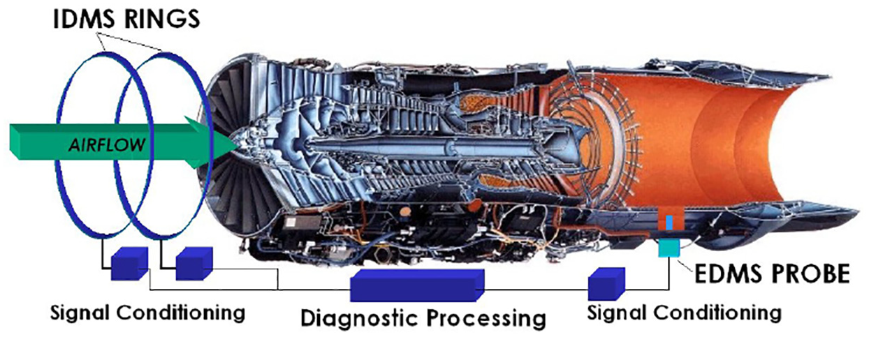
IDMS and EDMS.

The basic principle of electrostatic monitoring technology is electrostatic induction. When the particles pass through the rod-like probe, part of the electric field lines due to the charge terminate at the probe surface. The electrons in the probe are redistributed to balance the extra charge, creating a current that causes the appearance of a charge pulse signal. The principle is shown in Figure 2.

Figure 2.

The principle of electrostatic monitoring.

The overall layout of electrostatic sensor array equipped at the exhaust nozzle of aero-engine we design in this paper is shown in Figure 3:

Figure 3.

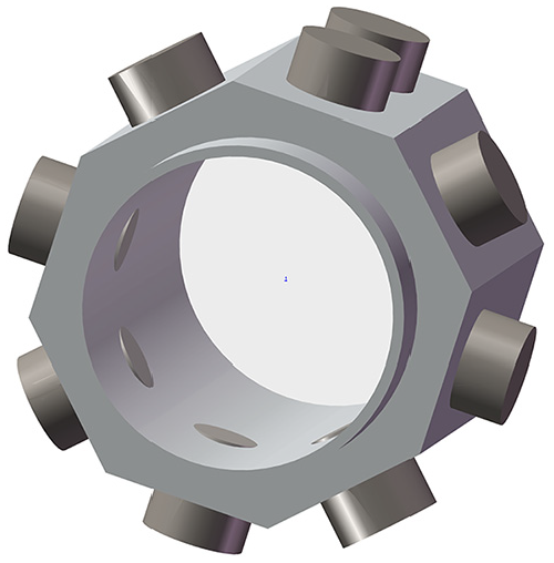
The overall layout of electrostatic sensor array.

There are nine rod-like probes installed on two cross sections in the exhaust nozzle. We use the signals from the eight rod-like probes in the front cross section to estimate the spatial position and charge amount of particle. The two axially adjacent spaced probes in the adjacent cross sections can be used to determine the velocity of particle.

The inner diameter of the circular pipe is 70 mm in this paper. The angle between each two probes is 45°. The length of probe’s side surface is 10 mm and the diameter of probe’s end surface is 15 mm. In order not to affect the inside of the circular pipe, we place nine probes at positions where they are just connected to the inner wall of the circular pipe. The depth of the probes inserted into the circular pipe is 0.813 mm according to the geometric relationship. The followed sections use the same parameters described here. It is necessary to note that the diameter of the circular pipe is just an example. Moreover, the inducing area of probe is an important factor. The larger the probe sensing area, the higher the induced charge amount on the probe according to Gauss Theorem. It is noted that we just take the sizes set in this paper as an example to verify the methods proposed in this paper. Obviously, larger area of aero-engine nozzle’s cross section needs larger probe area.

Analysis of planar array signal problem

Set the cross section which contains eight probes be MTN. V axis is perpendicular to MTN. T is the center point of the cross section. Spatial sensitivity is the crucial parameter to describe the sensing characteristic of electrostatic sensor. The ith probe’s spatial sensitivity can be defined as the ratio between induced charge amount Q_i on probe and particle’s charge amount q, induced charge amount Q_i means the amplitude of the induced charge signal on the probe. The ith probe’s spatial sensitivity is described in equation (1) when the particle is locating at the position (m, n):

$${\mathrm{S}}_i(m,n)=\left|\frac{{\mathrm{Q}}_i}{q}\right|$$

(1)

Apparently, the spatial sensitivity establishes the bridge between electrostatic sensors’ induced charge amount Q_i, the charge amount of particle q, and the spatial position of particle (m, n). Generally, it is hard to get the exact equation of S_i (m, n). Assume a particle is locating at the position (m, n), the ith probe’s induced charge amount can be expressed as equation (2) according to the principle of electrostatic induction:

$${\mathrm{Q}}_i=\int \underset{\mathrm{C}}{\int }\mathit{P}(m,n){\mathit{S}}_i(m,n)\mathrm{dmdn}$$

(2)

Where $C$ represents MTN plane, P (m, n) represents the charge distribution in MTN plane. The exact equation of S_i (m, n) cannot be obtained so we may get the discrete numerical solution of S_i (m, n) and rewrite equation (2) into the form of a discrete matrix:

$${\mathit{Q}}_s=\mathit{SP}$$

(3)

The problem of planar array signal in the cross section is to solve P when Q_s and S are known. S represents the discrete spatial sensitivity matrix of electrostatic sensor array in MTN plane and Q_s represents the measurement vector that contains the induced charge amounts on the electrostatic array’s eight probes in MTN plane. P is the charge distribution vector of the cross section MTN. Then we can further estimate particle’s spatial position and charge amount based on P.

How to get P is an inverse solution problem in the electrostatic field and is ill-posed. The uniqueness of the solution cannot be satisfied. The classic method to solve this problem is the regularization method. We choose the most widely used Tikhonov regularization to solve it in this paper. And we also introduce compressed sensing to solve this problem and compare it with Tikhonov regularization.

Before introduce Tikhonov regularization and compressed sensing, we need to establish the mathematical model and deeply analyze the induced principle to guarantee the correctness of the proposed methods. And then we use mathematical model to obtain the discrete spatial sensitivity S.

Mathematical model and numerical analysis

We establish a detailed mathematical model based on three-dimensional rectangular coordinate system. Figure 4 shows the electric field diagram of a particle with a charge amount of q as it passes near the rod-like probe. The sensing surface can be divided into an end surface and a side surface, and the sum of the charge amounts on the two surfaces is the total induced charge amount.

Figure 4.

The electric field diagram of particle.

Set the origin of the end surface center be O and establish a space coordinate system centered on O. Set a point F on the side surface and its coordinate is (u, v, w), set a point K on the end surface and its coordinate is (e, f, j). The electric field of K on the end surface is shown in Figure 5. Assume that the particle is in the spatial position G, and its coordinate is (x, y, z). Set the height of rod-like probe be L and the radius of end surface is R.

Figure 5.

Electric field of K on the end surface.

Most of the particles are above the end surface (z > 0). Assume that the particle whose charge amount is q at the spatial position G, G₀ is the projection of G. E_⊥ is the electric field intensity at point K. E_⊥ is the projection of E perpendicular to the end surface.

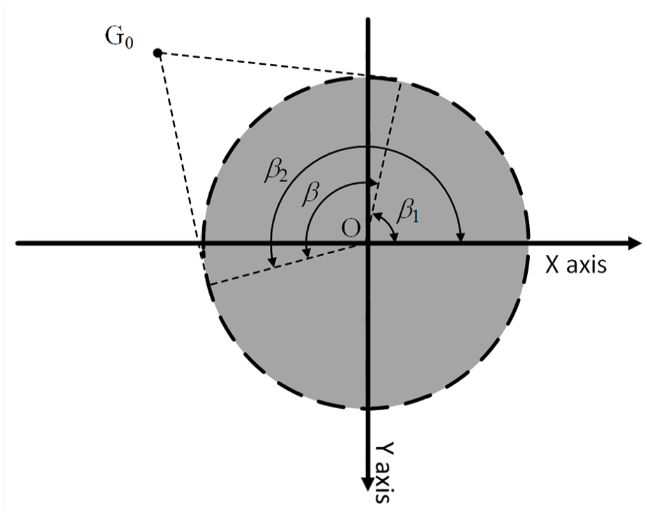
A schematic diagram of the effective sensing area on the side surface is shown in Figure 6. The effective angle of the particle on the side surface is the central angle of the tangents of G₀ and the circular section.

Figure 6.

The effective sensing area of side surface.

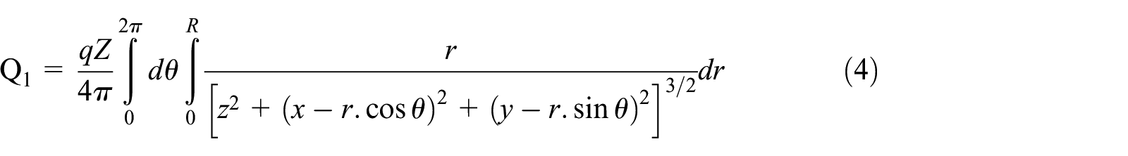
The total charge amount on the end surface can be obtained by integration:

$${\mathrm{Q}}_1=\frac{\mathrm{qZ}}{4\pi }\underset{0}{\overset{2\pi }{\int }}d\theta \underset{0}{\overset{R}{\int }}\frac{r}{{[z^2+{(x-r.\cos \theta )}^2+{(y-r.\sin \theta )}^2]}^{3/2}}\mathrm{dr}$$

(4)

The total charge amount on the side surface can be obtained by integration:

$$\begin{array}{c}\multicolumn{1}{c}{{\mathrm{Q}}_2=\frac{q}{4\pi }{\int }_{\arctan |\frac{y}{x}|-\arccos |\frac{R}{\sqrt{x^2+y^2}}|}^{\arctan |\frac{y}{x}|+\arccos |\frac{R}{\sqrt{x^2+y^2}}|}d\beta }\\ \multicolumn{1}{c}{{\int }_{-L}^0\frac{|R-|x|\cos \beta -|y|\sin \beta |}{{[{(z-w)}^2+{(|x|-R\cos \beta )}^2+{(|y|-R\sin \beta )}^2]}^{3/2}}}\end{array}\mathrm{Rdw}$$

(5)

The sum of the induced charge amount on the two surfaces Q_total is the total amount of Q₁ and Q₂. It is expressed in equation (6):

$$\begin{array}{c}{\mathrm{Q}}_{\mathrm{total}}=\frac{\mathrm{qz}}{4\pi }\underset{0}{\overset{2\pi }{\int }}d\theta \underset{0}{\overset{R}{\int }}\frac{r}{{[z^2+{(x-r·\cos \theta )}^2+{(y-r·\sin \theta )}^2]}^{3/2}}\mathrm{dr}+\hfill \\ \frac{q}{4\pi }{\int }_{\arctan |\frac{y}{x}|-\arccos |\frac{R}{\sqrt{x^2+y^2}}|}^{\arctan |\frac{y}{x}|+\arccos |\frac{R}{\sqrt{x^2+y^2}}|}d\beta {\int }_{-L}^0\frac{|R-|x|\cos \beta -|y|\sin \beta |}{{[{(z-w)}^2+{(|x|-R\cos \beta )}^2+{(|y|-R\sin \beta )}^2]}^{3/2}}\mathrm{Rdw}\hfill \end{array}$$

(6)

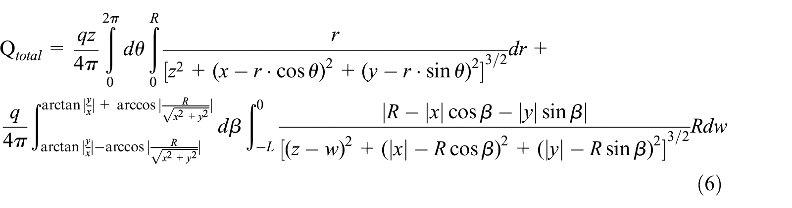
It is noted that the detailed calculation procedure of this mathematical model is described in our previous work and the correctness of this established mathematical model has been verified by the experiments. ³¹ Although the mathematical model does not take into account the dielectric constant of the material, our previous work ³¹ has proven that this will not bring much error. When the particle’s position is constant, the amount of induced charge on the probe obtained by the mathematical model is almost the same as the amount of induced charge on the probe under actual conditions. Combined with the definition of equation (1), this means that we can get a sufficiently accurate sensitivity distribution matrix based on the mathematical model.

The collected monitoring data is the voltage waveform in the experiments. As the crucial device, the charge amplifier used in the experiments should be introduced here. The induced charge signal on the probe is very weak. Therefore, before connecting to the acquisition card, the output charge signal of the electrostatic sensor needs to be conditioned by the charge amplifier. The charge amplifier is usually divided into two categories. One is to use resistance to collect inductive current signal. The other is to use operational amplifiers as the core to convert the charge signal to voltage signal and connect the feedback resistance and capacitance in the circuit to control the gain and band width.

If we choose the first type of charge amplifier, the collected voltage waveform will be the derivative of the charge waveform and reflects the rate of change of charge waveform as shown in Figure 7.

Figure 7.

The relationship between voltage and charge.

In order to make collected voltage waveform reflect the initial charge waveform instead of reflecting the derivative of charge waveform, we choose to use the second type of charge amplifier. When the gain is fixed, the magnification between the output voltage signal and the inductive charge signal on the probe is fixed.

We can obtain the induced charge amount of the rod-like probe when the particles are located at any spatial positions by equation (6). During the moving process, the moving particle continuously forms an induced charge on the probe, which constitutes the induced charge pulse waveform. This paper simulates the motion of the particle by the process of digital signal sampling with MATLAB and assume that the particle does a uniform linear motion. The modeling process is as follows:

1. Set the sampling frequency Fs be 40 kHz, the sampling interval ΔT is 0.025 ms.

2. Set the distance of the particle moves within ΔT be ΔL and we can change ΔL to simulate the change of velocity. For example, set ΔL be 0.025 mm means the velocity of the particle is 0.025/0.025 = 1 m/s. With this method, we can simulate particle moving in a straight line at any constant velocity.

3. Moving the particle along a direction parallel to the X-axis to simulate the process of particle passing through the probe. Change ΔL to simulate the movement of the particle passes through the probe at various velocities. It can be done in a multi-layer loop by MATLAB.

Keep particle’s spatial position and charge amount unchanged. Set v to 1, 2, 3 m/s for comparison and set particle at a certain spatial position and carry 1 pc. The induced charge pulse waveforms’ comparison is shown in Figure 8.

Figure 8.

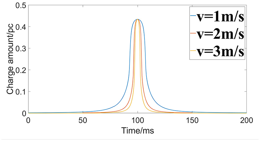
Induced charge waveform according to different particle’s velocities.

The amplitude of the charge pulse signal is the induced charge amount on the probe when the particle passes through the YOZ plane. It is obvious that the amplitude of induced charge signal does not change with the change of velocity. The induced charge amount will stay unchanged when the particle’s charge amount and spatial position are unchanged.

This crucial inducing characteristic is the fundament of the follow sections. It proves that the proposed method based on the eight probes’ induced charge amounts in the followed sections to estimate the spatial position and charge amount of particle is reasonable. Regardless of whether the velocity of the particle is same, as long as the particle with a certain charge amount passes the rod-like probes at the same spatial position, the amplitudes of induced charges on the probes will not change.

Electrostatic sensor array’s spatial sensitivity

We use the established mathematical model in the previous section to acquire the discretization matrix S of spatial sensitivity distribution.

To get the discrete spatial sensitivity matrix S, the MTN plane is discretized to 949 points. In other words, these 949 discrete points are used to describe the sensitivity distribution of the entire MTN plane.

There are eight probes in MTN plane so the dimension of S is 8 × 949. The measurement vector Q_s contains the amplitude of the induced charge on the eight probes so the dimension of Q_s is 8 × 1. The dimension of charge distribution vector P is 949 × 1.

It is noted that the XOY plane and Z axis in the mathematical model are not same with the MTN plane and V axis which are used to represent the cross section of circular pipe. The geometric relationship between the two coordinate systems is shown in Figure 9:

Figure 9.

The geometric relationship between two coordinate systems.

We need to use the coordinate relationship in Figure 9 to get S. There are eight probes and we take one probe as the example. The distance between center point on the probe’s end surface O and cross section’s center point T is 34.187 mm because depth of every probe inserted into the circular pipe is 0.813 mm as introduced in section 2.1. The angle t is the angle between the two coordinate systems. The angle between each two probes is 45°( $\frac{\pi }{4}$ ) so t can be expressed by equation (7):

$$t=(\mathrm{j}-1)·\frac{\pi }{4},\mathrm{j}=1,2...8$$

(7)

In equation (7), j means the jth probe.

Through the above translation and rotation, the coordinates of the points in the MVN coordinate system can be converted to the XYZ coordinate system for calculation.

Let the charged particle carry 1 pc to locate at the 949 discrete points to obtain the amplitude of induced charges on the eight probes. The amplitude now is just the spatial sensitivity according to the definition described in equation (1). Traverse all 949 discrete points then we can get the discretization matrix S (8 × 949) of spatial sensitivity distribution.

The normalized spatial sensitivity of one probe (one-eighth of matrix S) is shown in Figure 10:

Figure 10.

The normalized spatial sensitivity of one probe.

The normalized spatial sensitivity of one probe is distributed very unevenly in the cross section, and is only sensitive near the probe, which is not conducive to the measurement of the spatial position and charge amount of the particle.

The normalized spatial sensitivity of four probes who are 90° apart from each other (half of matrix S) is shown in Figure 11:

Figure 11.

The normalized spatial sensitivity of four probes.

Although it is also only sensitive near the probe, the spatial sensitivity of the four probes is about four times higher in the central region of the cross section than that of just one probe. In the areas between the four probes, the sensitivity is still very low with very small increase, and the probes are not sensitive to the changes in the position of particles in these areas. Therefore, it is not enough to estimate the spatial position and charge amount of particle just using four probes.

The normalized spatial sensitivity of eight probes who are 45° apart from each other (the whole matrix S) is shown in Figure 12:

Figure 12.

The normalized spatial sensitivity of eight probes.

It is clear to see that the spatial sensitivity is more even than that of four probes. This is beneficial to estimate the particle’s spatial position and the charge amount.

Principle of estimation methods

We need to get the charge distribution vector P and estimate the spatial position and charge amount of charged particle based on it as introduced in section 2.2. We introduce two methods to obtain P and compare their performance in section 4.

Tikhonov regularization principle

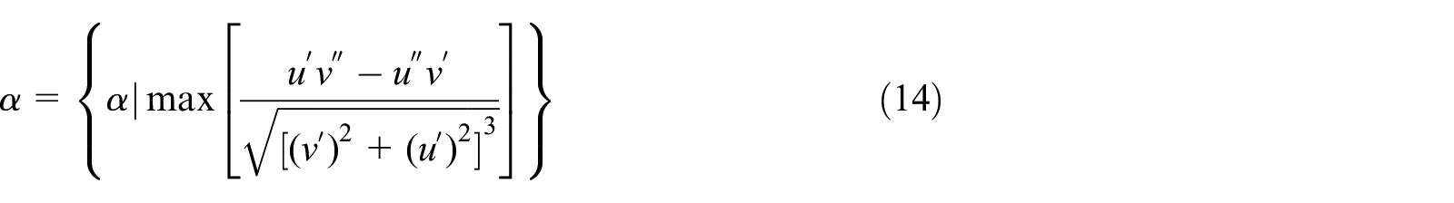
The essence of Tikhonov regularization algorithm is to use the best approximation principle based on least squares to calculate the best approximate solution. To get the best approximate solution $\stackrel{\wedge }{x}$ of an equation: Ax = y (where A is a matrix, x and y are vectors), $\stackrel{\wedge }{x}$ should satisfy:

$$\Vert \mathit{A}\stackrel{\wedge }{x}-y\Vert \le \Vert \mathit{A}x-y\Vert ,\forall x\in X$$

(8)

$\stackrel{\wedge }{x}$ is the solution of functional extremum problem $\underset{x\in X}{\min }\Vert \mathit{A}x-y{\Vert }^2$ . This problem is equivalent to solving the following equation:

$${\mathit{A}}^{*}\mathit{A}x={\mathit{A}}^{*}y$$

(9)

${\mathit{A}}^{*}$ is the conjugate transpose of A. The method of adding a penalty term is used to solve the ill-posed problem when solving the above extremum problem according to the optimization theory. The problem of solving $\stackrel{\wedge }{x}$ can be transformed into equation (10):

$$\underset{x\in X}{\min }(\Vert \mathit{A}x-y\Vert +\alpha \Vert x{\Vert }^2)$$

(10)

Where α is the regularization parameter. Set ${\mathit{J}}_{\alpha }=\Vert \mathit{A}x-y\Vert +\alpha \Vert x{\Vert }^2$ and J_α is called Tikhonov function. Solving the solution x_α of equation (10) is equivalent to solving the unique solution of equation (11):

$${\mathit{A}}^{*}\mathit{A}{x}_{\alpha }+\alpha x_{\alpha }={\mathit{A}}^{*}y$$

(11)

Equation (12) can be obtained from equation (11):

$$x_{\alpha }=({\mathit{A}}^{*}\mathit{A}+\alpha \mathit{I}{)}^{-1}{\mathit{A}}^{*}y$$

(12)

In equation (3), Q_s is a vector consisting of the measured charge amplitude of eight probes, S represents the sensitivity matrix of electrostatic sensor array in the cross section and plays the role of sensing matrix, and P is a vector that consist the information of induced charge distribution. For the specific problem of solving the charge distribution vector P when Q_s and S are known in this paper, P can be calculated by equation (13) according to equation (12):

$$\mathit{P}=-({\mathit{S}}^{*}\mathit{S}+\alpha \mathit{I}{)}^{-1}{\mathit{S}}^{*}{\mathit{Q}}_s$$

(13)

We adopt the L curve method, which is highly robust to autocorrelation noise, to determine the regularization parameter α:

$$\alpha =\{\alpha |\max \left[\frac{u^{\prime }{v}^{″}-u^{″}{v}^{\prime }}{\sqrt{{[{(v^{\prime })}^2+{(u^{\prime })}^2]}^3}}\right]\}$$

(14)

Where $u=\Vert \mathit{S}\stackrel{\wedge }{\mathit{P}}-{\mathit{Q}}_s\Vert ,v=\Vert \stackrel{\wedge }{\mathit{P}}\Vert$ .

Compressed sensing principle

The compressed sensing (CS) theory treats a sparse signal to be measured as an N-dimensional sparse vector c. In signal acquisition, CS theory uses an M × N-dimensional (M $<<$ N) sensing matrix Θ to directly compress c into an M-dimensional measurement vector d as shown in equation (15). This compression process can retain enough information to reconstruct the sparse vector x under certain conditions, and then only need to solve a sparse optimization problem to accurately reconstruct x from y precisely.

$$d=\Theta c$$

(15)

In equation (15), the sensing matrix Θ should satisfy restricted isometry property (RIP). It is a necessary condition for c to be reconstructed correctly. Therefore, the problem expressed by equation (3) can be solved by the principle expressed by equation (15), too.

The key technical detail is how to preprocess sensitivity matrix S to satisfy RIP condition. The method based on singular value decomposition (SVD) is adopted to preprocess equation (3) to make the processed sensing matrix S_svd in the equation satisfy the RIP condition.

According to the SVD theory, the sensitivity matrix S is a full row rank, which can be decomposed as in equation (16).

$$\mathit{S}=\mathit{U}\left[\begin{array}{cc}\mathit{\Delta }\hfill & 0\hfill \end{array}\right]{\mathit{V}}^{\mathrm{T}}$$

(16)

Where U is the orthogonal matrix of 8 × 8 and V is the orthogonal matrix of 949 × 949. Δ = diag (δ₁, δ₂, …, δ _M ), where δ₁ ≥ δ₂ ≥ … ≥ δ _M  > 0 are all M singular values of S.

Let Δ^* = diag (1/δ₁, 1/δ₂, …, 1/δ _M ) and Z = Δ^*U^TS, then the processed Q_ssvd can be defined as equation (17).

$${\mathit{Q}}_{\mathrm{ssvd}}={\mathit{\Delta }}^{*}{\mathit{U}}^T{\mathit{Q}}_{\mathrm{s}}={\mathit{\Delta }}^{*}{\mathit{U}}^T\mathit{SP}=\mathit{ZP}$$

(17)

Z can be simplified to equation (18) by applying the principle of equation (16).

$$\mathit{Z}={\mathit{\Delta }}^{*}{\mathit{U}}^T\mathit{S}={\mathit{\Delta }}^{*}{\mathit{U}}^T\mathit{U}\left[\begin{array}{cc}\mathit{\Delta }\hfill & 0\hfill \end{array}\right]{\mathit{V}}^{\mathrm{T}}=\left[\begin{array}{cc}\mathit{I}\hfill & 0\hfill \end{array}\right]{\mathit{V}}^{\mathrm{T}}$$

(18)

It is convenient to use equation (18) to calculate Z, then unitize each column of Z, and use the obtained matrix as the processed sensitivity matrix S_svd, as shown in equation (19).

$${\mathit{S}}_{\mathrm{svd}}=\mathit{Z}\left[\begin{array}{cccc}1/{\Vert z_1\Vert }_2\hfill & 0\hfill & \cdots \hfill & 0\hfill \\ \multicolumn{1}{c}{0}& 1/{\Vert z_2\Vert }_2\hfill & \cdots \hfill & 0\hfill \\ \multicolumn{1}{c}{⋮}& ⋮\hfill & \ddots \hfill & ⋮\hfill \\ \multicolumn{1}{c}{0}& 0\hfill & \cdots \hfill & 1/{\Vert z_n\Vert }_2\hfill \end{array}\right]$$

(19)

Where z₁, z₂, …, z_n are the column vectors of Z. And then equation (20) can be inferred out.

$$\mathit{Z}={\mathit{S}}_{\mathrm{svd}}\left[\begin{array}{cccc}{\Vert z_1\Vert }_2\hfill & 0\hfill & \cdots \hfill & 0\hfill \\ \multicolumn{1}{c}{0}& {\Vert z_2\Vert }_2\hfill & \cdots \hfill & 0\hfill \\ \multicolumn{1}{c}{⋮}& ⋮\hfill & \ddots \hfill & ⋮\hfill \\ \multicolumn{1}{c}{0}& 0\hfill & \cdots \hfill & {\Vert z_n\Vert }_2\hfill \end{array}\right]$$

(20)

Define P_svd as equation (21) shows, and substitute equations (21) and (20) into equation (17). Then equation (22) can be obtained.

$${\mathit{P}}_{\mathrm{svd}}=\left[\begin{array}{cccc}{\Vert z_1\Vert }_2\hfill & 0\hfill & \cdots \hfill & 0\hfill \\ \multicolumn{1}{c}{0}& {\Vert z_2\Vert }_2\hfill & \cdots \hfill & 0\hfill \\ \multicolumn{1}{c}{⋮}& ⋮\hfill & \ddots \hfill & ⋮\hfill \\ \multicolumn{1}{c}{0}& 0\hfill & \cdots \hfill & {\Vert z_n\Vert }_2\hfill \end{array}\right]\mathit{P}$$

(21)

$${\mathit{Q}}_{\mathrm{ssvd}}={\mathit{S}}_{\mathrm{svd}}{\mathit{P}}_{\mathrm{svd}}$$

(22)

S _svd is a partly orthogonal matrix meets the condition of RIP. Therefore, P_svd can be correctly inversed, and then P can be obtained by using equation (21).

Solving the sparse solution of equation (15) needs to satisfy the constraint of l₀-minimization. What’s more, there is a need to say that l₀-minimization is an ideal constraint to figure out a group of sparse solutions which have the fewest nonzero elements. However, solving l₀-minimization directly is a non-deterministic polynomial hard (NP-hard) problem. CS theory believes that under certain conditions, l₀-minimization problem can be transformed to l₁-minimization problem to solve the sparse solutions of equation (15). The primal-dual interior point method which is contained in CVX toolkit in MATLAB can be used to solve l₁-minimization problem.

The verification experiments

To verify the effectiveness of the supposed method, we establish two test rigs. All sizes are same with the descriptions in sections 2 and 3. The actual object of the model shown in Figure 3 is shown in Figure13.

Figure 13.

The electrostatic sensor array and the circular pipe.

Oil calibration test rig

To verify if electrostatic sensor array has the ability to estimate particle’s spatial position and charge amount, we establish the oil calibration test rig.

We use the oil drop to simulate the particle. As Figure 14 shows, the test rig consists of an oil drop generation section, a sensor support position section, an electrostatic signal acquisition section, and an oil drop charge measurement section.

Figure 14.

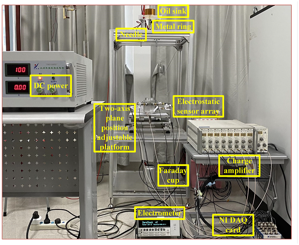
The oil calibration test rig.

When the rig works, the oil in the oil sink enters the high voltage electric field formed by the metal needle and the metal ring. Under the action of the high voltage electric field, the oil drops will carry certain charge amount. The high voltage electric field strength can be adjusted by the adjustable DC power, the maximum output voltage is 700 V. The charge amount of oil drop is proportional to the output voltage of DC power. Therefore, the test rig can adjust the charge amount through changing the output voltage of DC power linearly.

The sensor support and position section can accurately adjust the relative position between the sensor and the drop path through the two-axis platform’s slide rail. The altitude of sensor array can also be adjusted to change the oil drop’s velocity.

The induced charge signals of the probes will be converted to voltage signal by the charge amplifier and then collected by NI acquisition card as introduced in section 2.3.

The charge measurement section measures the exact charge amount of the oil drops by a Faraday cup which is connected to KEITHLEY 6517B electrometer.

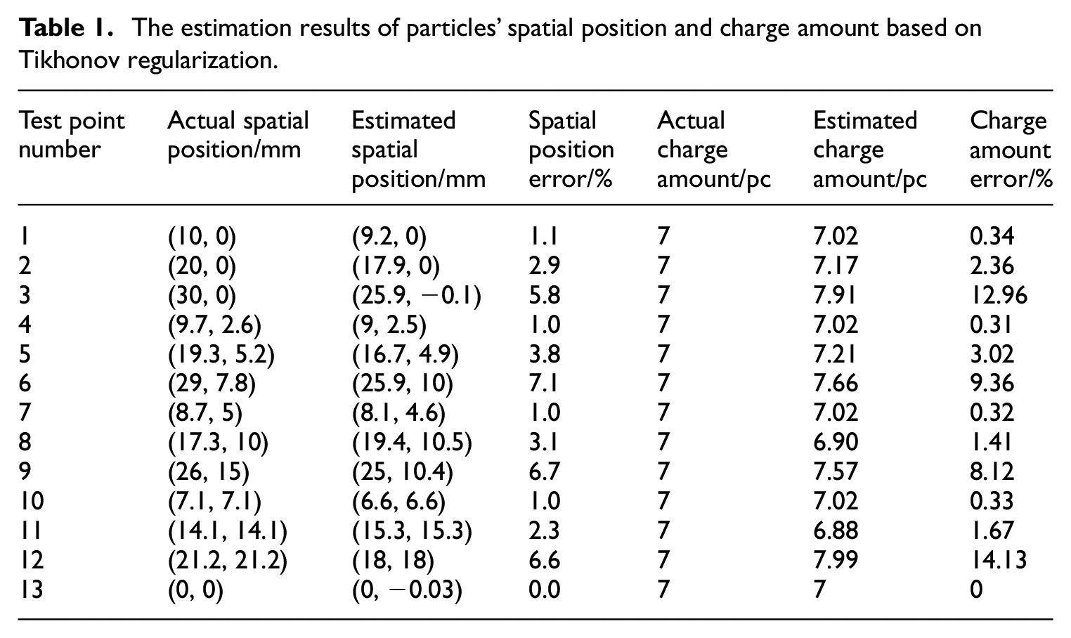
We know that the angle between each two probes is 45° in this paper. The electrostatic sensor array layout is symmetrical so we just need to select some test points within 45°. As shown in Figure 15, we select 13 test points. Their coordinates are listed in the second column of Tables 1 and 2.

Figure 15.

The spatial positions of test points.

Table 1.

The estimation results of particles’ spatial position and charge amount based on Tikhonov regularization.

Test pointnumber	Actual spatialposition/mm	Estimatedspatialposition/mm	Spatial positionerror/%	Actualchargeamount/pc	Estimatedchargeamount/pc	Chargeamounterror/%
1	(10, 0)	(9.2, 0)	1.1	7	7.02	0.34
2	(20, 0)	(17.9, 0)	2.9	7	7.17	2.36
3	(30, 0)	(25.9, −0.1)	5.8	7	7.91	12.96
4	(9.7, 2.6)	(9, 2.5)	1.0	7	7.02	0.31
5	(19.3, 5.2)	(16.7, 4.9)	3.8	7	7.21	3.02
6	(29, 7.8)	(25.9, 10)	7.1	7	7.66	9.36
7	(8.7, 5)	(8.1, 4.6)	1.0	7	7.02	0.32
8	(17.3, 10)	(19.4, 10.5)	3.1	7	6.90	1.41
9	(26, 15)	(25, 10.4)	6.7	7	7.57	8.12
10	(7.1, 7.1)	(6.6, 6.6)	1.0	7	7.02	0.33
11	(14.1, 14.1)	(15.3, 15.3)	2.3	7	6.88	1.67
12	(21.2, 21.2)	(18, 18)	6.6	7	7.99	14.13
13	(0, 0)	(0, −0.03)	0.0	7	7	0

Table 2.

The estimation results of particles’ spatial position and charge amount based on compressed sensing.

Test pointnumber	Actual spatialposition/mm	Estimatedspatialposition/mm	Spatialpositionerror/%	Actual chargeamount/pc	Estimatedchargeamount/pc	Chargeamounterror/%
1	(10, 0)	(9.7, −0.2)	0.5	7	7.01	0.13
2	(20, 0)	(18.8, −0.4)	1.9	7	7.10	1.40
3	(30, 0)	(23.6, −0.6)	9.2	7	8.32	18.87
4	(9.7, 2.6)	(9.3, 2.4)	0.5	7	7.01	0.15
5	(19.3, 5.2)	(18.7, 5.3)	0.9	7	7.04	0.57
6	(29, 7.8)	(27.8, 10.3)	4.0	7	7.15	2.21
7	(8.7, 5)	(8.4, 4.8)	0.5	7	7.01	0.15
8	(17.3, 10)	(17, 9.4)	1.0	7	7.04	0.60
9	(26, 15)	(27.1, 12)	4.6	7	7.17	2.48
10	(7.1, 7.1)	(6.8, 6.9)	0.4	7	7.01	0.12
11	(14.1, 14.1)	(13.1, 13.5)	1.8	7	7.10	1.40
12	(21.2, 21.2)	(16.3, 16.9)	9.3	7	8.33	18.93
13	(0, 0)	(0, −0.06)	0.1	7	7	0

Adjust the position section of the oil test rig to let the oil drops fall from the 13 selected positions. The slide rail and the scale feet on the two-axis position platform can help us regulate the positions. Adjust the DC power to let the oil drops carry 7 pc. As explained in sections 2 and 3, the amplitudes of the induced charges on the eight probes constitute the measurement vector Q. The spatial sensitivity matrix S has been obtained. The estimated spatial positions and the estimated charge amounts of the oil drops can be got according to the charge distribution vector P that can be calculated through Tikhonov regularization and compressed sensing. The detailed calculation procedure are as follows:

1. Collect eight probes’ amplitudes of output voltage signals in each experiments. Then multiply the amplification factor of the charge amplifier to get the inducing charge amount to obtain the measurement vector Q whose the dimension is 8 × 1;

2. Get the charge distribution vector P (949 × 1) by using Q (8 × 1) and S (8 × 949) through Tikhonov regularization or compressed sensing explained in section 3;

3. Set $p_i\in \mathit{P}(i=1,2,...,949)$ . Eliminate data that does not meet the Pauta criterion and remain m data that meet Pauta criterion. Now $p_i\in \mathit{P}(i=1,2...m)$ , which means there are only m points remaining in the 949 points;

4. Calculate the weight w_i of p_i:

$$w_i=\frac{p_i}{\sum _1^m{p}_i}$$

(23)

• (5) Set the x coordinate of point i be x_i (i = 1, 2, …, m) and the y coordinate of point i be y_i (i = 1, 2, …, m);

• (6) Calculate the estimated x coordinate of the test point be Xt:

$$\mathrm{Xt}=\sum _i^m{x}_i{w}_i$$

(24)

Calculate the estimated y coordinate of the test point be Yt:

$$\mathrm{Yt}=\sum _i^m{y}_i{w}_i$$

(25)

Now we can get the estimated spatial position of the test point by combining the x coordinate and the y coordinate: (Xt, Yt);

• (7) We have the measurement vector Q which contains the amplitudes of the inducing charge amount of eight probes, and we know the spatial sensitivity S of the MTN plane and the estimated spatial position. Therefore, we can get eight estimated charge amounts of the oil drop. The eight estimated values are averaged to get the final estimated charge amount Qt;

• (8) Set the actual spatial position of the test point be (Xa, Ya) and set the actual charge amount be Qa. The inner diameter of the circular pipe is 70 mm. We can get the estimated spatial positon error errorP and the estimated charge amount error errorQ through equations (26) and (27):

$$\mathrm{errorP}=\left(\frac{\sqrt{{(\mathrm{Xt}-\mathrm{Xa})}^2+{(\mathrm{Yt}-\mathrm{Ya})}^2}}{70}\right)·100\mathrm{\%}$$

(26)

$$\mathrm{errorQ}=\left|\frac{\mathrm{Qt}-\mathrm{Qa}}{\mathrm{Qa}}\right|·100\mathrm{\%}$$

(27)

• (9) Repeat the above steps to get all the estimated spatial positions and estimated charge amounts of every experiments.

It is worth noting that the mathematical model abstracts the charged particles as point charges, while the oil drops in the experiments have certain volume and their charges are distributed on the surface of the oil drops. We assume that the charge on the surface of the oil drop is evenly distributed. The charge of the oil drop is gathered to the centroid of oil droplet based on this assuming. However, the charge of the oil drops cannot be completely uniformly distributed on the surface in the actual condition. This systematic error will have a certain impact on the accuracy of the estimation results, and it is inevitable. In order to minimize the inherent systematic error, we repeat the experiments at every test points and then take the average values.

The second step is the core of all nine steps because all the remaining steps are based on the charge distribution vector P, which reflects the charge distribution in the MTN plane (the cross section of circular pipe) according to different test points. There is a need to say that we do not show the raw signals in this section because they are similar with the signals show in the next section. Therefore, we just show the calculated results in Figure 16 and the tables.

Figure 16.

The charge distribution obtained by Tikhonov regularization according to: (a) test point 1, (b) test point 5, (c) test point 9, and (d) test point 13.

We select the charge distribution vectors obtained by Tikhonov regularization of 4 test points out of all the 13 test points for display:

The estimation results based on Tikhonov regularization are shown in Table 1:

We can see that the estimation errors of particle’s spatial positions and particle’s charge amounts based on Tikhonov regularization are both higher when the particles are closer to the wall. Although the estimation errors of spatial positions do not exceed 10% when the particles are close to the wall, the estimation errors of charge amounts at same spatial positions could exceed 10%. The closer to the wall, the more uneven the spatial sensitivity. This phenomenon can be seen from Figures 10 to 12. At the positions close to the wall, small changes in position will cause sudden changes in spatial sensitivity. The extremely uneven spatial sensitivity distribution is the most important factor affecting the accuracy of particle charge amount estimation.

We also select the charge distribution vectors obtained by compressed sensing of 4 test points out of all the 13 test points for display, too:

The estimation results based on compressed sensing are shown in Table 2:

It is obvious that the charge distribution obtained by compressed sensing is sparser than that obtained by Tikhonov regularization from Figure 17. We can see that the estimation errors of particle’s spatial positions and particle’s charge amounts based on compressed sensing are both higher when the particles are closer to the wall, too. On the whole, the estimation accuracy calculated by compressed sensing is higher than Tikhonov regularization except test point 3 and test point 12.

Figure 17.

The charge distribution obtained by compressed sensing according to: (a) test point 1, (b) test point 5, (c) test point 9, and (d) test point 13.

Then we verify electrostatic sensor’s ability to determine the particle’s velocity by using the ninth probe and its front probe. The velocity can be calculated directly from the measured raw dual-channel signals of the two probes with cross-correlation algorithm. The specific steps are as follows:

• (1) Through cross-correlation calculation, the number of sampling points DelayN between the dual-channel signals of the two probes are obtained.

• (2) In this paper, we set the sampling frequency Fs be 40 kHz. Calculate the delay time between dual-channel signals:

$$\mathrm{DelayT}=\frac{\mathrm{DelayN}}{\mathrm{Fs}}$$

(28)

• (3) The distance DelayD of the ninth probe and its front probe is 35 mm. Calculate the velocity of the oil drop:

$$V=\frac{\mathrm{DelayD}}{\mathrm{DelayT}}$$

(29)

Adjust the height of the oil sink and the needle to let the oil drops fall with different velocities under the action of gravity. Let the oil drops fall from the heights H of 500, 600, and 700 mm respectively. The actual velocities Vg when the oil drops pass the electrostatic sensor array are 3.13, 3.43, and 3.70 m/s respectively according to the acceleration of gravity. Calculate the oil drops’ estimated velocity Vc by the method we describe above and the results are shown in Table 3. We can see that there are almost no errors between the estimated velocities and the actual velocities. This is also consistent with the conclusion of our previous work, ³¹ too. But we need to emphasize that this only applies to the case of single particle. In the case of multi particles, whether cross-correlation can accurately estimate the velocity still needs further research.

Table 3.

The estimation results of particles’ velocities.

H/mm	Vg/m·s−1	Vc/m·s−1	Error/%
500	3.13	3.1	0.9
600	3.43	3.39	1.2
700	3.70	3.65	1.4

Air-gun test rig

We verify electrostatic sensor array’s ability to estimate the spatial position and charge amount and then calculate the velocity of particle in the previous section. However, the oil calibration test rig has two limitations: (1) It cannot simulate different kinds of particles such as metal particles and non-metal particles; (2) It cannot simulate the condition of high velocity. The two main disadvantages make the oil test rig unable to simulate the actual working condition of aero-engine. Therefore, we carry out further experiments based on an air-gun test rig. The sampling frequency Fs is 40 kHz, too. In this test rig, we use the small ball to simulate the particle.

As shown in Figure 18, the air pump is used to provide adequate gas pressure. The protective box is used as a container to accept the ball to avoid hurting people. The core components of the air gun are three valves and an air pressure regulator. To launch a ball, these four components need to cooperate with each other and operate according to a certain process.

Figure 18.

The air-gun test rig.

The air pressure regulator in the pipeline is used to regulate gas pressure from 0 to 1 MPa. Different air pressures push balls to be emitted with different velocities. The knob on the regulator can be continuously adjusted to regulate the air pressure and the pointer can clearly display the air pressure. The three valves are intake valve, exhaust valve, and ball launch valve. Firstly, we close the other two valves and only open the intake valve, let the air flow from the air pump go into the pipeline, and adjust the air pressure regulator to obtain different air pressures. Secondly, we close the other two valves and only open the exhaust valve, release the airflow in the pipe and put the small ball into the pipeline. After that, we close the bleed valve and open the intake valve again to let air flow into the pipeline. Finally, we open the ball launch valve and let the ball shoot out.

Firstly, we use it to verify electrostatic sensor array’s ability to distinguish metal particles and non-metal particles because there are many different particle sources in the aero-engine.

We shoot a 5 mm iron ball at a certain spatial position under certain air pressure. The measured raw signals of the eight probes are shown in Figure 19:

Figure 19.

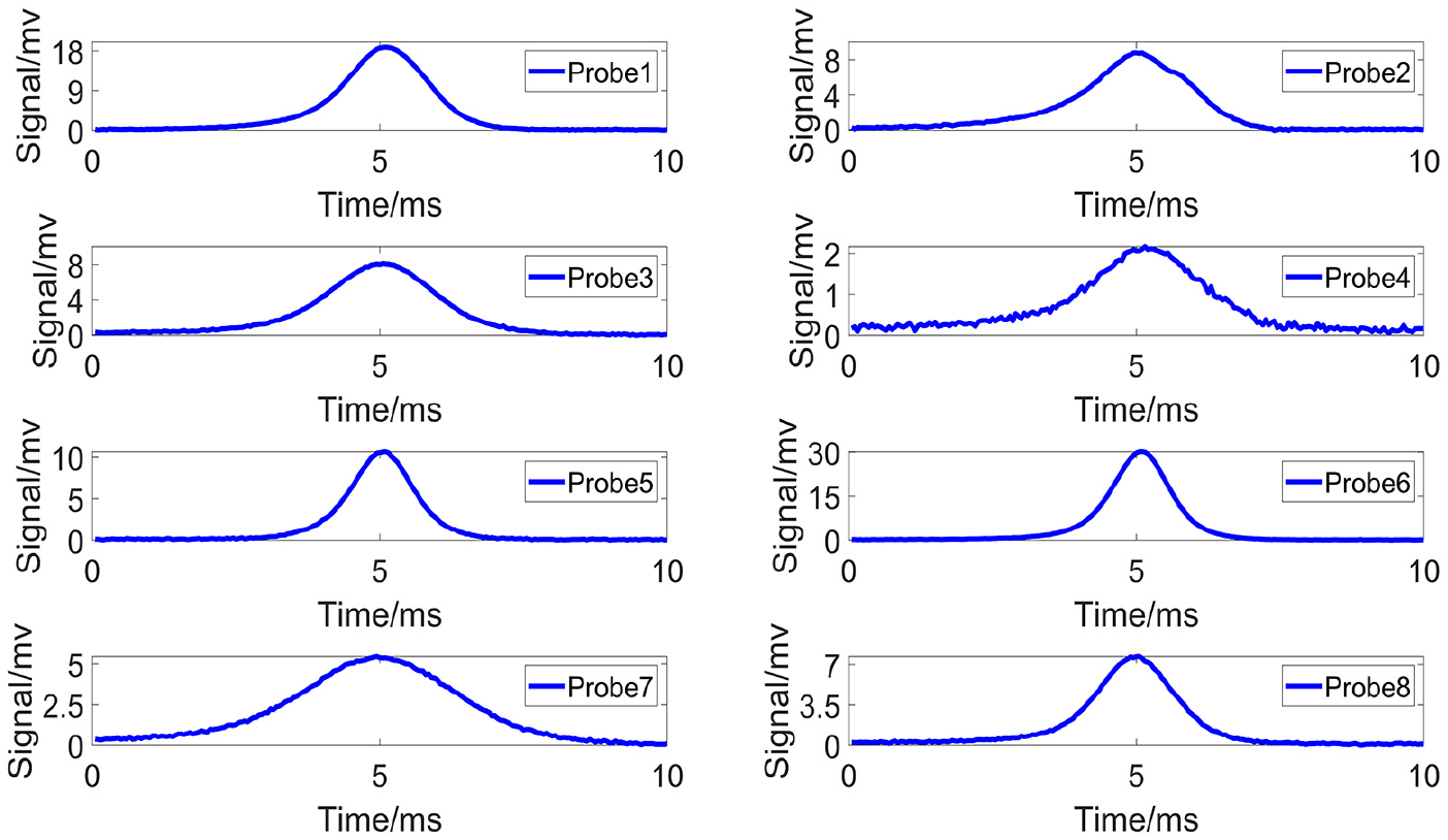
The measured raw signals of electrostatic sensor array when ingested a metal object.

We can see that the induced signals on the probes show positive polarity when the metal particle passes by because metal particles are positively charged after friction with air.

We shoot a 5 mm PTFE (Poly tetra fluoro ethylene) ball at a certain spatial position and under certain air pressure. The measured raw signals of the eight probes are shown in Figure 20:

Figure 20.

The measured raw signals of electrostatic sensor array when ingested a non-metal object.

We can see that the induced signals on the probes show negative polarity when the non-metal particle passes by because non-metal particles are negatively charged after friction with air.

What’s more, Figures 19 and 20 show another interesting phenomenon: The induced pulse signal’s width is relative to the particle’s spatial position. When the charge amount and velocity of particle are same, the farther the particle is from the probe, the smaller the induced charge amount on the probe but the farther the particle is from the probe, the larger the pulse width of the induced signal. This is proved in our previous work. ³¹

Secondly, we use this air-gun test rig to simulate the high velocity movement. Considering safety, we adjust the air pressure to 0.5 MPa and calculate particle’ velocity by using Dual-channel cross-correlation algorithm introduced in section 4.1, too.

Shoot PTFE ball at a certain spatial position and the measured raw dual-channel signals are shown in Figure 21:

Figure 21.

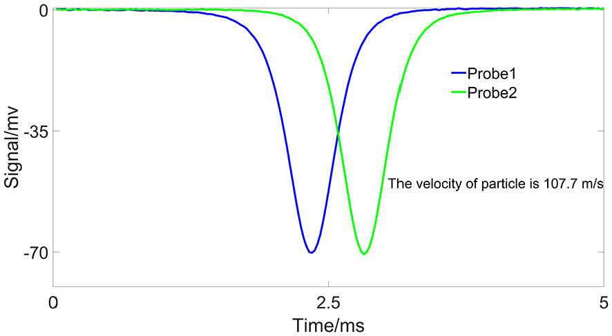
The dual-channel signals.

The calculated velocity is 107.7 m/s. The gas pressure can be adjusted from 0 to 1 MPa and we don’t try the pressure more than 0.5 MPa because it is dangerous. The particle can have the velocity of more than 100 m/s by only adjusting the pressure to 0.5 MPa. We verify the accuracy of cross-correlation in the previous section so the result is credible. It is enough to prove the air-gun test rig has the ability to simulate the high velocity condition. Electrostatic sensor can monitor particle with high velocity.

Conclusions

In this work, we establish a mathematical model to analyze the inducing characteristics of electrostatic sensor and get the spatial sensitivity distribution. Tikhonov regularization and compressed sensing are applied to estimate the spatial positon and charge amount of particle. The estimation errors of spatial position and charge amount are both higher when particles are closer to the wall. The velocity of particle can be calculated directly from the measured raw dual-channel signals with cross-correlation algorithm. The oil calibration test rig is established to verify these theories and methods. The further experiments are taken on an air-gun test rig to further simulate the high velocity conditions and verify electrostatic sensor’s ability to distinguish the metal and non-metal particles.

There are some following issues to be solved in the future:

• (1) We just verify the feasibility of the proposed method and only analyze the signals in ideal conditions but the actual conditions of aero-engine are very complicated. There is a need to carry out experiments on the real aero-engines.

• (2) There are many particles in the gas exhaust of aero-engine and we just study the case of a single particle in this paper. The induced charge signal of the multi-particles is the superposition of single particle’s induced signal. Further theoretical analysis and experimental verification are required for the estimation of charge amount of multi particles. We hope this study could be the foundation of the future work about multi particles.