Sage Journals: Discover world-class research

Abstract

We demonstrate a method for the fast in vivo quantification of small volumes, down to 25 µL, using low-field magnetic resonance imaging (MRI) coils. The coils were designed so as to maximize the signal-to-noise ratio (SNR) in the images. For this we developed an analytical model for describing the variations of the SNR with coil design and with size/shape suited to the object under observation. Based on the conclusions drawn from the model, the coil parameters were chosen in order to reach an SNR close to the maximum. For the validation of the model, coils were finally characterized in terms of quality factor using saline phantoms. The coil design procedure is illustrated here with two examples: first, the quantification of about 200 µL of intradermal injected gel on rabbits with a single loop surface coil and second, the imaging of the intervertebral disks in rat tails using a small volume coil to detect possible lesions. Such studies would not have been feasible for the clinical low-field MRI system at our disposal using any of the commercially available medium-sized manufactured coils. As a result of this simple optimization procedure, a wide range of applications is accessible even at low magnetic fields, leading to new opportunities for low-cost, though efficient, preclinical studies.

Keywords

low-field MRI coil optimization non-invasive small animal sacrifices reduction

Preclinical studies usually result in the sacrifice of a high number of animals. But preclinical imaging, especially preclinical magnetic resonance imaging (MRI), offers an attractive non-invasive alternative. Animals can be followed in vivo in longitudinal studies, thus allowing the number of animals needed to be reduced.¹ For most studies, small animals such as rodents or lagomorphs are used. But preclinical imaging using a clinical whole body MRI using the commercial coils that come with the system is not always optimal. This is especially the case if none of the coils amongst the set of coils provided by the manufacturer of the MRI device properly matches the animal shape. Moreover, third party companies do not always offer commercial dedicated coils for small or medium-sized animal imaging in clinical MR systems. Examinations of small animals are often performed over small regions of interest (ROI), and only a weak signal is available with a non-dedicated coil, especially at low magnetic field strengths (below 0.5 Tesla [T]). Even if preclinical imaging focused on small animals employs dedicated high magnetic field MRI (4.7 T, 7 T or higher), these MR systems are expensive and are not always accessible in institutions.² Moreover, the overall gain in image quality is not as high as expected.^3,4 Image quality at clinical low fields (e.g. 0.2 T or 0.4 T) has been proven to be suitable for small animal studies when optimized coils were employed.^1,4 The advantages of clinical low-field systems are that the open architecture offers the possibility of performing interventional surgery. They also lead to a reduction in set-up times and are less hazardous with regard to magnetostatic forces. Moreover, no specific absorption rate (SAR) issues, which cause tissue heating, are reported, and less susceptibility artifacts are observed. This study offers an alternative to the preclinical imaging of rodents currently performed on high-field preclinical or clinical systems, by employing an inexpensive 0.18 T open magnet designed for human extremities. The cost of this system is three to six times lower than that of clinical wide bore systems (1.5 T and 3 T). Besides the low initial cost, the maintenance cost for a low-field permanent magnet is almost insignificant, notably because of the absence of power consumption and cryogenic fluids in the magnet. This clinical low-field system is also most suited for animals such as lagomorphs, due to its open magnet and its 200 mm × 200 mm × 200 mm static field and radiofrequency (RF) excitation field homogeneous region. In this work, two specific in vivo preclinical applications were assessed, and a dedicated coil was designed for each application. First a circular-shaped loop surface coil was built to quantify intradermic volumes of gels (∼200 µL) injected into rabbit dermis. Intradermal follow-up is usually performed by histology measurements which require the euthanasia of animals at regular time intervals during the study.^5,6 Although the use of ultrasound imaging has been reported,^7,8 MR is a non-invasive alternative for tracking the volume of intradermal injections. A similar study has been notably reported using an expensive 1.5 T clinical MRI device.⁹ Secondly, a volume coil was developed to image the tail of the rat in order to observe intervertebral disks and to further detect potential lesions. The degeneration of the caudal intervertebral disks is frequently monitored using MRI.^10–12 But this kind of study is usually performed using clinical or preclinical high-field MRI devices (>3 T). Low-field MR was therefore envisaged for this study as well as for the lagomorph study.

Materials and methods

Animals

The preclinical study on a rabbit model was requested by a third party institution for the commercialization of a hyaluronic gel designed for plastic surgery. The experimental protocol complied with all animal welfare guidelines, and with the regulations on animal experimentation (Directive 86/609/EC, amended by decree 87-848, decrees 2001-464 and 2005-264) and the recommendations of the Council of Europe Convention EST123. Five New Zealand White adult female rabbits (Charles River Laboratories International, Inc, Wilmington, MA, USA) with a mean weight of 3.5–4 kg were housed in the Claude Bourgelat Institute (VetAgro Sup, Lyon, France). Each of the five rabbits was injected in the dermis over eight sites with four different hyaluronic acid gels, one control reference gel and three gels under test. MR (followed by image processing for volume calculation) of all 40 intradermal injection sites was performed on day 0 (d0, injection), day 28 (d28) and day 84 (d84). The rabbits were anaesthetized during the MRI examinations using 1% isoflurane pushed by air with a cone-shaped head holder. The rabbits lay in a left decubitus position and their body temperature was maintained with hot water bottles.

The caudal disks were imaged in vivo on a Wistar Unilever adult rat. The animal lay in a prone position during the MR acquisitions and was anaesthetized with a 1% isoflurane/air mix with a well-adjusted cone-shaped head holder. Its body temperature was maintained with a hot water bottle on contact with the end of the tail.

Instruments

An MRI E-scan XQ device (Esaote, Genova, Italy) with an open permanent magnet and vertical static magnetic field of magnitude | B ₀| = B₀ = 0.18 T (f₀ = 7.78 MHz) designed for human extremities was used for both studies. The transmit-only coil was a saddle coil embedded into the device. Gradient coils which were available were able to reach amplitudes up to 20 mT/m, which made high spatial resolution imaging accessible (higher than 1 pixel/mm in each direction). Receive coils at our disposal were separate from the transmit coil on this MRI device and were decoupled from each other with a passive and/or a geometric method. The dedicated coils which were designed in the present paper employed either two axial-leaded 1N5819 Schottky or two surface-mounted DH80055 PIN crossed diodes (Temex Ceramics, Pessac, France) for decoupling. Decoupling of the receive coil during RF pulses from the transmit coil was needed to avoid image distortions.¹³

Coil optimization

With the commercial coils available in the clinical low-field MR system, small ROI could not be explored in acquisition times compatible with in vivo examinations. This was due to the small level of signal available in a reduced ROI, especially in low-field MRI. Two studies were consequently carried out: first on a surface coil, because for some applications it is crucial to obtain as much signal as possible over a reduced ROI at the skin surface, rather than to get an image of the whole body with an average signal-to-noise ratio (SNR);¹⁴ secondly on a volume coil for which the shape of the coil embraces the volume of the sample. For both coils, the design process was divided into three steps: mathematical modeling for the optimization of coil performance, coil fabrication, and finally electrical characterization based on electronic parameters to check performance and validate the model.

Mathematical model

The SNR intrinsic to an MRI coil was first described by Hoult¹⁵ as in (Eq. 1):

SNR \propto \frac{| B_{1 r} |}{\sqrt{R_{eq}}}

(1)

where B _1r (T/A) is the current sensitivity of the coil (dependent mainly on coil geometry) and R_eq (Ω) is an equivalent resistance in series with the inductance which summarizes overall loss phenomena occurring in the coil (e.g. a larger coil has a higher R_eq).¹⁶ B _1r is the field induced by a unit current flowing in the coil by reciprocity.¹⁶ At low fields and thus long wavelengths, a quasistatic approach (the Biot–Savart law) remains accurate for estimating B _1r.^16,17 Integration using the Biot–Savart law was performed numerically using MATLAB (The MathWorks, Inc, Natick, MA, USA) over volumes or surfaces specified by the constraints of the study. During the MRI experiment, the amplitude of the signal collected by the receive coil originating from a specific location was maximized when B _1r at the center of the coil was orthogonal to B ₀ at this location. If B ₀ is arbitrarily oriented such that B ₀ = B₀· y and is considered as perfectly homogeneous in both strength and direction, only the x and z components of B _1r _, B_1x and B_1z are considered. In (Eq. 1), | B _1r| becomes B_1xz:¹⁸

B_{1 xz} = \sqrt{B_{1 x}^{2} + B_{1 z}^{2}}

(2)

For some applications, for example in volume coils, an image with the most constant signal over a given region is needed. As a consequence, it is useful to evaluate the maximum deviation of the collected MR signal in this region thanks to the principle of reciprocity.¹⁵ Assuming that the sample is homogeneous and that the RF field produced by the transmit-only coil is also homogeneous over this volume, the spatial variations of the collected MR signal are caused only by the spatial variations of sensitivity in the receive coil. We therefore introduce the maximum relative deviation Δ of B_1xz as:¹⁸

Δ = max (\frac{B_{1 xz} (r_{0}) - B_{1 xz} (r_{1})}{B_{1 xz} (r_{0})})

(3)

with r ₀ as a reference point and r ₁ a point in the field of view (FOV) of the coil which maximizes the deviation. For volume coils, Δ is calculated on the z axis.¹⁸ Thus, r ₀ refers to the center of the coil where B_1xz is at a maximum, and r ₁ is the coil boundary on the axis where B_1xz is at a minimum. This definition was extrapolated to surface coils: at a given surface distance z₀, the maximum deviation of B_1xz in a plane parallel to the coil is easily computed. This plane is bounded to the projected edges of the coil. With this definition of Δ for surface coils, r ₀ and r ₁ respectively refer to the points of maximum and minimum for B_1xz at depth z₀.

For the estimation of R_eq, the schematic of Figure 1 includes the various elements involved. This equivalent circuit was needed for the estimation of R_eq and subsequently for the calculation of the SNR variation (Eq. 1).

Figure 1.

Electronic circuit of a low-field magnetic resonance imaging (MRI) device (coupling capacitors not shown). (a) All the individual loss phenomena are illustrated: R_coil and R_leads are the losses in the coil itself, R_m and R_d are losses caused respectively by the magnetic and dielectric losses in the sample, and R_dec and R_ct are the losses in the electronic components (respectively the decoupling diodes and the tuning capacitor). (b) The equivalent parallel RLC circuit. (c) The hybrid equivalent circuit which includes the equivalent series resistance R_eq required for the estimation of the signal-to-noise ratio (SNR). For circuit (c), the series inductance is almost identical to that in parallel, provided that the quality factor Q₀ of the coil (R_eqP/ω₀ * L_eqP) is much larger than unity. Then R_eq = R_eqP/(1 + Q₀²) with Q₀ = ω₀ * L_eq/R_eq. The equations used for the calculation of all parameters are reported in Appendix A.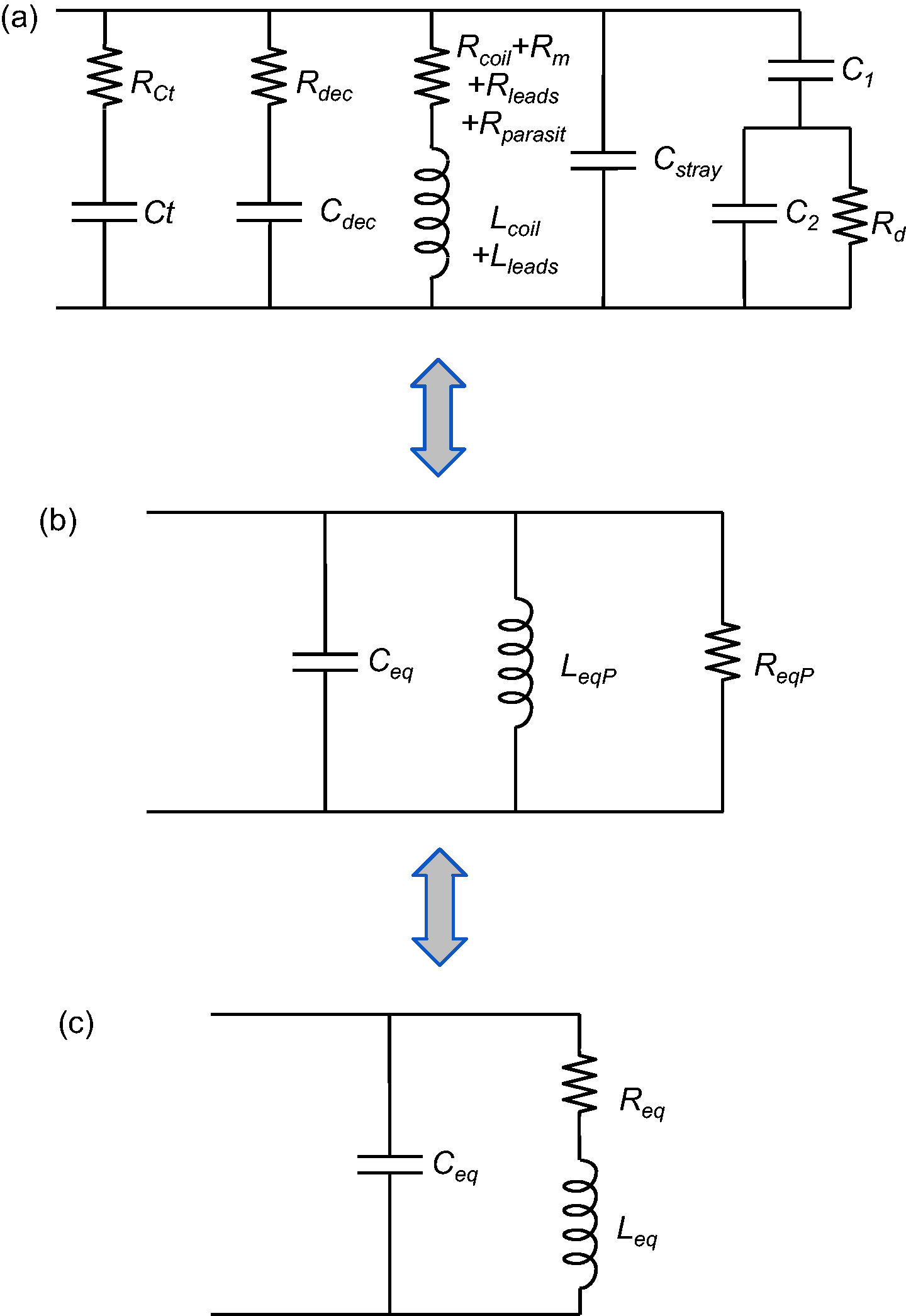

The overall noise sources can be described by various contributions¹⁹ (see Appendix A): the losses in the coil itself (R_coil), the losses in the sample under observation (R_sample which is subdivided into two distinct phenomena: the magnetic losses R_m and the dielectric losses R_d) and finally the losses in the electronic components (such as the tuning capacitors R_ct and decoupling diodes R_dec).^16,20–22 The losses in the coupling capacitors can be ignored if the coil is tuned and matched at f₀.²⁰ The losses in the coaxial cable can be ignored as well. These two assumptions were confirmed by circuit simulations in LTspice (Linear Technology, Milpitas, CA, USA) and ANSYS HFSS (ANSYS Inc, Canonsburg, PA, USA). At f₀ = 7.78 MHz, the wavelength is about 39 m in air and 1.35 m in muscle,²³ which were much greater than coil or sample dimensions in our studies. The radiation losses were consequently considered negligible. For the same reason, the equivalent electronic circuit of Figure 1 was valid. Apart from these considerations, every loss phenomenon needs to be taken into account at this working frequency.^16,24–26 Thus, coil and sample losses for medium-sized (1–10 cm diameter) coils are of the same order of magnitude, by contrast with the high-field experiments where sample losses or even tuning capacitor losses can become significant.^16,21,26 At B₀ = 0.18 T, a substantial increase in SNR is therefore achievable in theory by reducing coil losses, i.e. by optimizing receive coil design. In order to identify and avoid the main contributions of SNR degradation in our MR experiments, an exhaustive modeling of the losses as well as of the coil sensitivity map were necessary (Eq. 1).^15,20

For a given FOV, constrained by the sequence parameters and hardware characteristics, and for any given object or ROI which needs to be examined with its specific shape and size, the geometry of the coil is usually chosen either for filling factor (and thus SNR) maximization or for minimization of Δ. Once the geometry has been determined, a compromise between R_eq reduction and B_1xz increase (Eq. 1) can be achieved by adjusting the remaining free geometrical parameters of the coil (such as the number of turns in a solenoid or conductor thickness). This compromise is not always straightforward, since increased sensitivity can be obtained at the expense of increased losses.²⁷ Simulations using a simple though exhaustive SNR model are therefore valuable for the optimization of the design of a coil dedicated to a specific application.

Concerning the study on rabbit dermis, a dedicated receive surface coil was designed so as to image and quantify the intradermal gel volumes. Single circular loop geometry was initially chosen for this application because of the shape of the sample whose projection on the dermis and coil plane (x0y, see Figure 2) was circular, but egg-shaped on an orthogonal plane (x0z for example). The circular coil was compared to a square coil with a side equal to the diameter of the circular coil. The values of SNR and Δ were estimated for both surface coils. The SNR was estimated on the axis z of the coil, at depth z₀ which stood for the maximum extent of the injection into the dermis of the rabbit. The calculation of B_1xz maximum relative deviation Δ, using Eq. 3, was computed along a line parallel to the x axis at z = z₀ (see Figure 2a). The radius a of the loop was first constrained by the ROI which was a 15 mm wide injection. Consequently, the coil radius was at least 8 mm. Secondly, the maximum depth z₀ of about 10 mm also determined the loop radius for the best examination affordable in the dermis. Indeed, the SNR at depth z = z₀ was maximized by choosing the best a value. The SNR variation for a simple circular geometry was well described by Suits et al.²⁸ in 1998. They considered the case of a semi-infinite medium with negligible dielectric sample losses. However, for a complete understanding of the various noise contributions, SNR was expressed here using Eq. 1 and Appendix A. The coil sensitivity B_1xz of the circular-shaped coil was calculated over the x0z plane with –20 mm < x < 20 mm and 0 mm < z < 25 mm. Figure 2 illustrates the results of the simulations both for the spatial (Figure 2a) and parametric variations of B_1xz (Figure 2b).

Figure 2.

(a) x0z map of the surface coil signal-to-noise ratio (SNR), normalized against SNR(x = 0, z = z₀) and calculated over −20 mm < x < 20 mm and 0 mm < z < 25 mm (the surface coil is oriented in the x0y plane). The extent of the injection conditions the sensitivity map of the coil so that it includes the whole site. Given that the injection has a diameter of about 15 mm (see dashed egg-shape), then the radius a of the coil is at least 8 mm. The location of the 1.5 mm diameter conductor of the coil is represented by the two circles at x = ±10 mm and z = 0 mm, although the simulations employed a linear model for the conductor. Normalized SNR values are bounded to [0; 3] for visibility purposes since B_1xz increases strongly at the vicinity of the conductor. The maximum relative deviation Δ of B_1xz was computed along the horizontal dashed line at z = z₀ = 10 mm with −a < x < a. (b) Normalized theoretical SNR (in arbitrary units) as a function of parameter a (coil radius) at several depths z₀ along z axis: 5 mm, 10 mm, 15 mm, 20 mm and 25 mm from top to bottom. z₀ is defined as the deepest extent of the injection along z, which was about 10 mm on rabbits. SNR was normalized relatively to the SNR for a = 10 mm and z₀ = 10 mm which was the optimum for the intradermal study (thick curve maximum). The points of the maxima for each observation depth z₀ are drawn at the top of each curve. ROI: regions of interest.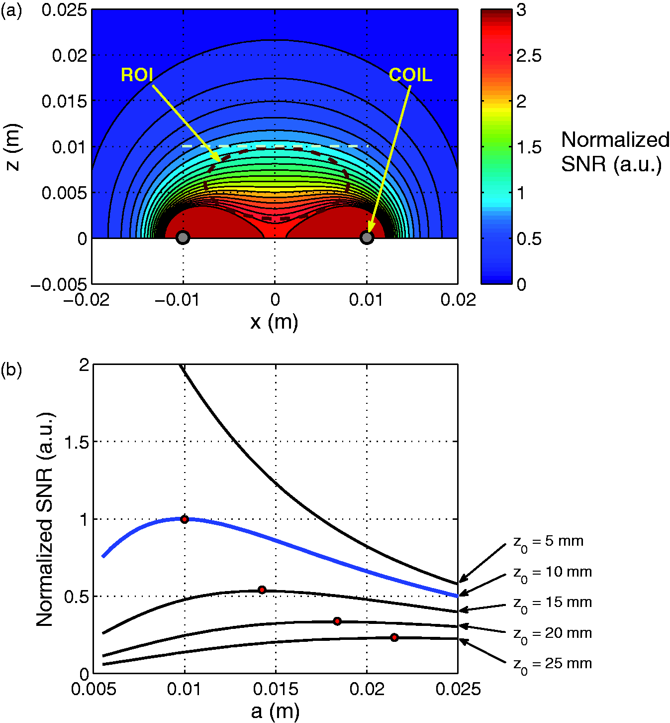

The SNR of a circular surface coil strongly depends on the radius as expected.¹⁴ As observed in Figure 2b, SNR(a) for a given depth z₀ shows a maximum for a unique a_opt value. The dots on each curve of Figure 2b stand for the maxima of SNR(a) for various observation depths z₀. For z₀ = 10 mm, we found that a_opt was ∼10 mm. The B_1xz map (Figure 2a) confirms that for such dimensions, the coil includes in its FOV the whole injection site (dashed ellipse). According to complementary simulations at depth z₀ on the axis of a square coil with a side of 20 mm the SNR was 9% higher, whereas Δ was 25% lower compared to a circular coil with a radius of 10 mm. Yet, the SNR on the axis at z = 0 was 19% better for the circular coil. Although a circular geometry was chosen initially, these simulations suggest that for this application, a square-shaped coil would be a good alternative offering slightly better performances. The wire was chosen as the thickest available in the laboratory for R_coil minimization, i.e. dw = 1.5 mm. This diameter is the maximum for enameled copper wire available at most electronic retailers. Although 2 mm is also available, the goal of this paper was to allow for the in-house design of low-field RF coils using off-the-shelf materials, so this copper wire was employed.

Concerning the study on caudal intervertebral disks, MR of the rat tail was performed in order to observe disk quality and identify potential lesions for preclinical studies in which caudal disk regeneration in rats would be followed.¹² According to the shape and size of the tail, the most appropriate coil geometry was a cylindrical volume coil. With vertical low static field B ₀, the coil type allowing for the best intrinsic SNR and lowest Δ is of a solenoid type.^1,15,29,30 As a compromise between Δ and SNR performances needed to be reached, variations of both relative to the design parameters of the coil were undertaken. The four parameters for a solenoid-shaped coil are the length L of the solenoid, the radius R of the solenoid (distance from conductor center to solenoid axis), the wire thickness dw, and the number of turns n. On the one hand, the SNR model was derived from Eq. 1, for which R_eq was estimated as in Appendix A. On the other hand, Δ was calculated between the points at r ₀ = {0, 0, 0} (the center of the solenoid) and r ₁ = {0, 0, L/2} (the edge of the solenoid)¹⁸ (Figure 4a). The parametric variations of Δ and SNR are illustrated in Figure 3. Each was obtained as a function of one of the four parameters of the coil, the remaining three being set to arbitrary values (those used in the final design of the coil).

Figure 3.

Normalized signal-to-noise ratio (SNR) and maximum relative deviation Δ of B_1xz for a solenoid when: (a) length L varies; (b) radius R varies; (c) wire thickness dw varies; (d) number of turns n varies. The SNR was normalized against the final design which is L = 45 mm, R = 11.75 mm, dw = 1.5 mm and n = 10. The constants are: the radius Rs, the length Ls and the dielectric properties of the sample under observation.

Figure 4.

Map of: (a) the well-known spatial variation of B_1xz, and thus of the signal-to-noise ratio (SNR) in a solenoid-shaped coil over the x0z plane; (b) the parametric SNR at the center of the solenoid-shaped coil against the parameters n and dw, with L = 45 mm and R = 11.75 mm. The set of parameters (n, dw) of the final design is represented by the round dot at (n = 10, dw = 1.5 * 10⁻³ m). SNR values were normalized against the SNR for this design. The upper-right striped area is excluded because of the constraint upon n, dw and L, which is n * dw < L.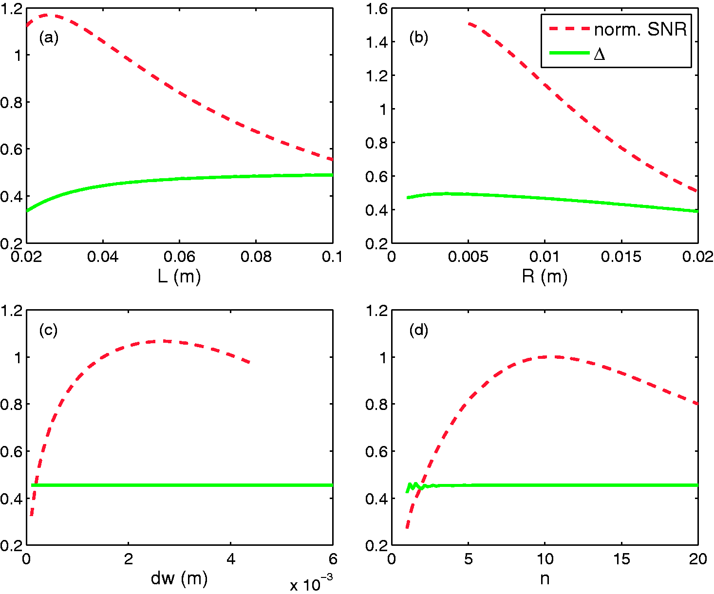

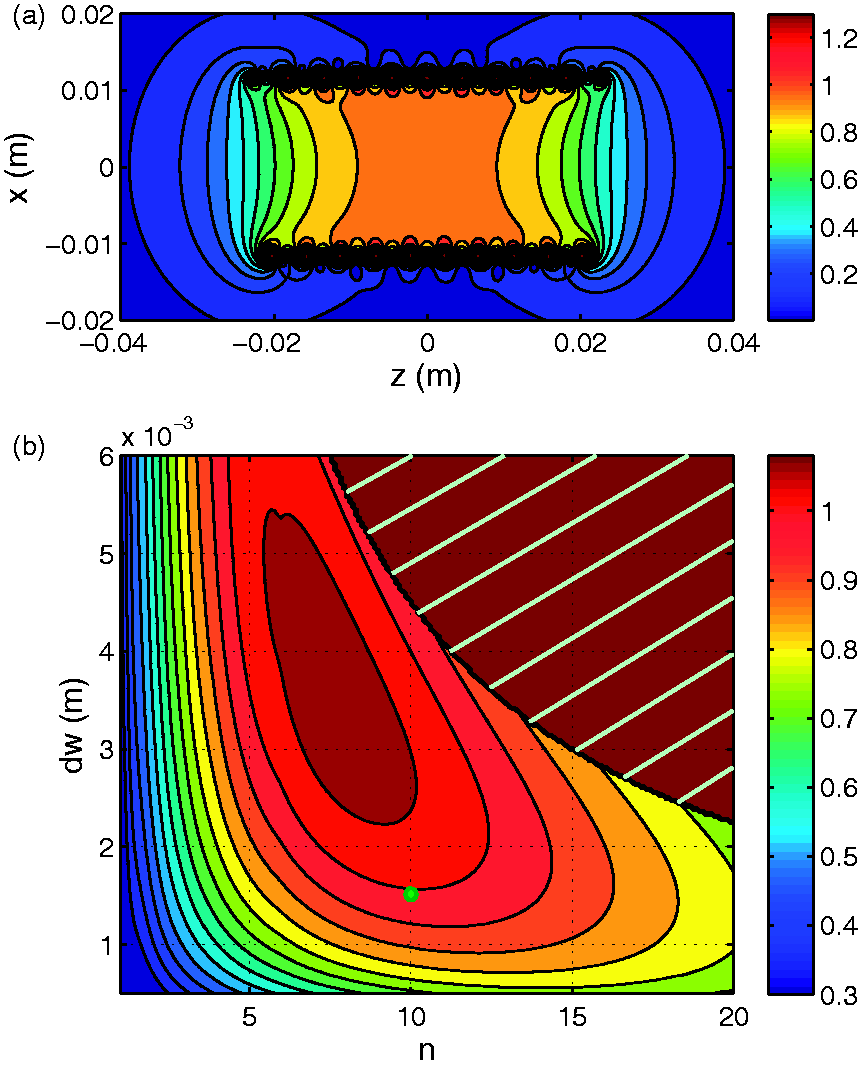
According to the model (Figures 3c and 3d), Δ depends only on the length L and the radius R of the solenoid, and these two parameters were set first. The radius R of the coil was fixed at 11.75 mm, given the diameter of the tail was up to 15 mm, which allowed a 1.5 mm air margin on both sides for ease of insertion and took into consideration the thickness of the coil’s plastic holder (namely 2 mm on both sides, which gives an inner diameter of 18 mm). Two non-successive intervertebral disks were injured by a needle in previous studies,^10,12 consequently a length L, allowing an FOV over a ROI with five vertebrae, was found to be practical for observing two non-successive disks simultaneously. A good compromise between Δ and SNR performance was achieved if the length of the solenoid L was approximately equal to the length of the ROI (Figure 3a). We finally set L at 45 mm (Figure 4a). At this point, two free parameters remained: n and dw. The SNR variation versus n and dw in Figure 4b indicated that the best SNRs would be achieved with thick wire (dw between 2 mm and 5 mm) and a limited number of turns (n between 7 and 11) for an SNR within 10% of the optimum.

With the dw = 1.5 mm wire, only n could finally be adjusted. The best value of n for these three constrains was n = 10, as is illustrated in Figure 3d and Figure 4b. For this design, the map of the spatial variations of B_1xz is presented in Figure 4a.

Coil fabrication

For the surface coil, the conclusions of the model led to the design of a circular-shaped coil with a = 10 mm and dw = 1.5 mm for the best SNR at a depth z₀ = 10 mm. A picture of the completed surface coil is shown in Figure 5a.

Figure 5.

Constructed coils for: (a) rabbit intradermal study (surface coil); (b) rat tail intervertebral disks observation (volume coil).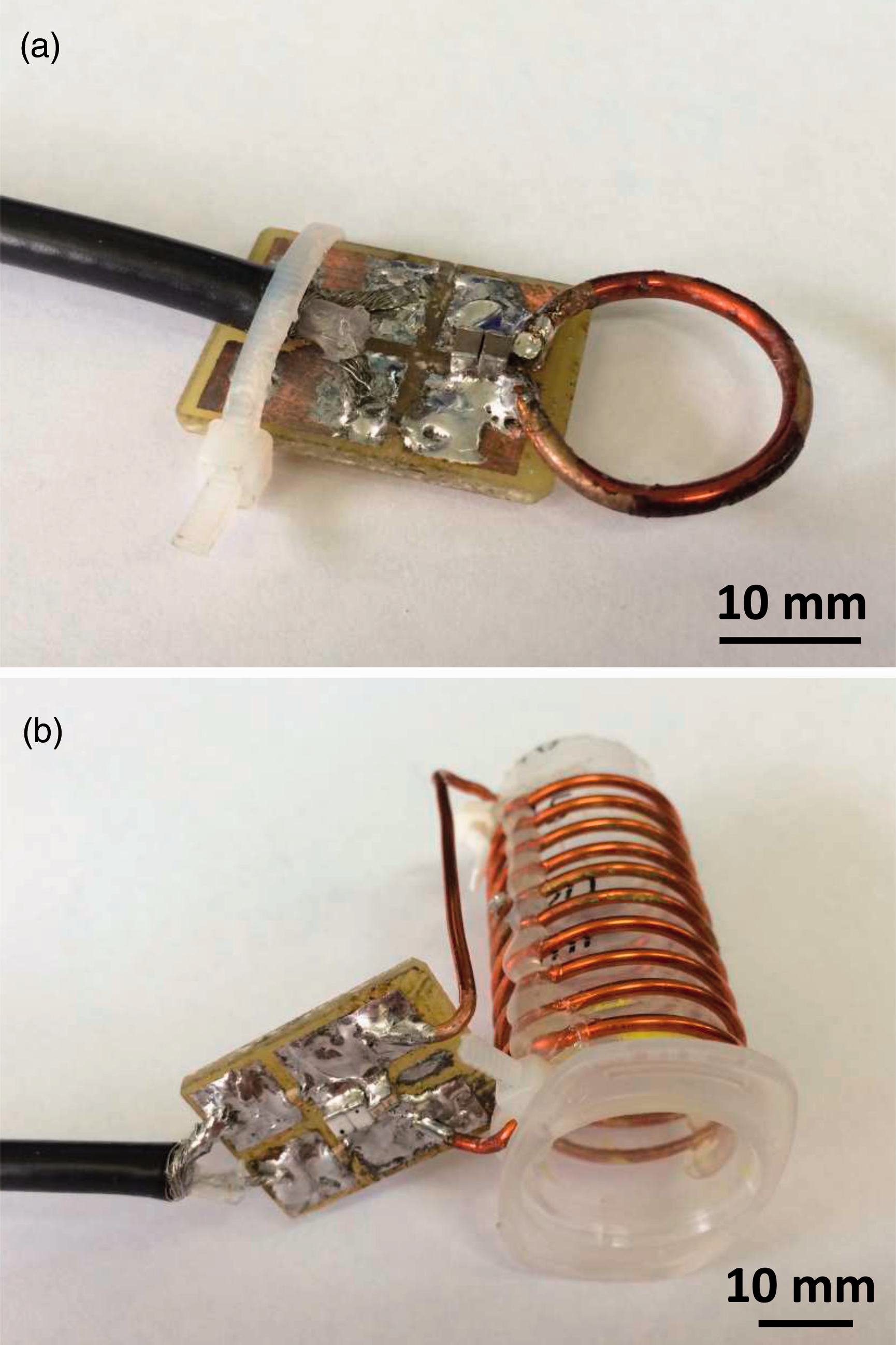

Figure 5b illustrates the constructed volume coil. The regularity of space between two consecutive turns was achieved by manually winding a plastic wire along with the copper conductor wire before applying glue. Once the glue was dry, the plastic wire was removed.

For the electronic part of the surface and volume coils, the tuned impedances (without the matching capacitors) were respectively 8.9 + j * 128 Ω and 6.6 + j * 965 Ω. Tuning at f₀ = 7.78 MHz (with C_t) and matching at Z₀ = 50 Ω (with C_m) – the transmission line characteristic impedance – were performed by ATC (American Technical Ceramics, Huntington Station, NY, USA) case ‘100A’, ‘700A’ or ‘100B’ (for high capacitance components) non-magnetic ceramic/porcelain capacitors (Figure 5 and Appendix A). A symmetric pattern was chosen for the matching network in order to reduce dielectric sample losses, especially for the volume coil.^21,31,32 Signal transmission was provided by a one-meter long RG58 coaxial line with non-magnetic BNC connectors (Radiall, Aubervilliers, France). To avoid excitation field inhomogeneity, the experiments with the small surface coil were set up in order to achieve a geometrical decoupling in addition to the passive decoupling diode, because the signal induced in the loop during transmit pulses was too weak. This coil orientation was manageable due to the open architecture of the MRI magnet and the vertical B ₀ orientation. However the size of the volume coil was sufficient for the induction of a sufficiently high voltage across the decoupling diodes during transmit pulses.

A +36 dB low noise (1.3 dB) preamplifier AU-1466 from Miteq (Miteq Inc, Hauppauge, NY, USA) was inserted between the coil and the MRI device to increase the signal of interest, thus minimizing parasitic noise. The amplifier was kept outside B ₀ for proper working, namely around 500 mm away from the center of the magnet.

Electrical characterization

When tuned and matched on a vector network analyzer (VNA) E5071 model from Agilent (Agilent Technologies, Santa Clara, CA, USA), quality factor measurements were performed to characterize the coils at room temperature (22℃) either when unloaded (Q_meas,_U) or loaded (Q_meas,_L) with a phantom. Quality factors Q_meas,_U_/_L were measured with the VNA on scattering parameter S11(f) curves over the Smith chart using a dedicated MATLAB script. This program was able to accurately estimate Q_meas and the coupling coefficient κ between the coil and the VNA as a result of an effective procedure. When the coil was either unloaded (index ‘U’) or loaded (index ‘L’) with the phantom, the actual quality factors of the disconnected coil (unplugged from the VNA), Q₀_,_meas,_U and Q_0, _meas, _L could be deduced from the measured values Q_meas_,U and Q_meas,L through:³³

Q_{0, meas, U} = (1 + κ) \cdot Q_{meas, U} Q_{0, meas, L} = (1 + κ) \cdot Q_{meas, L}

(4)

If impedance matching is lossless and perfectly adjusted to Z₀, the coupling coefficient κ is 1, and we confirmed the well-known fact that Q₀ _,meas is twice Q_meas. In this particular case, Q₀ _,meas is twice the ratio between the peak frequency f₀ and its bandwidth Δf at –3 dB.^3,30 Phantom loading was obtained with a 0.45% NaCl solution phantom adapted to the coil type (a 10 mL tube for the volume coil, and a 170 mm × 170 mm × 170 mm parallelepiped filled with an ∼4.9 L solution for the surface coil). This phantom has electrical properties which simulate living tissues, especially muscle properties (relative permittivity ɛ’ ∼ 208, conductivity σ ∼ 0.61 S/m).²³

For a comparison between the measurements and the SNR model, Q₀ _,calc,U/L values were calculated according to the estimation of the electrical components depicted in Figures 1c and 1b as:

Q_{0, calc, U} = \frac{ω_{0} L_{eq}}{R_{eq, U}} and Q_{0, calc, L} = \frac{ω_{0} L_{eq}}{R_{eq, L}} Or : Q_{0, calc, U} = \frac{R_{eqP, U}}{ω_{0} L_{eqP}} and Q_{0, calc, L} = \frac{R_{eqP, L}}{ω_{0} L_{eqP}}

(5)

MRI

A validation study was performed in vitro prior to the experiments on the rabbits in order to assess the accuracy and repeatability of the volume quantification using MRI. This validation study consisted of the MR acquisition of a microtube filled with a 100 µL volume of water using a 200 µL micropipette, followed by volume quantification. The volume measurement procedure (including acquisition and quantification) was repeated nine times by the same operator for an estimation of the repeatability while the accuracy was calculated as the difference between the measured and expected volumes. The surface coil was then compared to a commercial volume coil from the device manufacturer (a quadrature receive-only knee coil) both in vitro (on a saline phantom) and in vivo (on an injected rabbit) in terms of SNR. The SNR was measured as the mean value of the signal in the ROI divided by the standard deviation of the signal in the background of the image.³⁴ The coil was set close to each injection site of each rabbit (Figure 6a).

Figure 6.

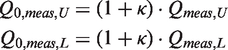
Acquisition and volume measurement steps for the rabbit study. (a) Magnetic resonance imaging (MRI) of each site with a 3D gradient echo sequence (TR = 26 ms, TE = 10 ms, NEX = 2, FA = 85°, matrix = 256 × 256 × 52/FOV = 130 mm × 130 mm × 31.2 mm). (b) MRI of an injection site obtained with the dedicated surface coil. (c) Gel surface segmentation (in red, see online version for colour version) using a threshold-based method. (d) Volume calculation and 3D rendering.

For SNR characterization, both the commercial knee volume coil (Figure 7e) and the designed surface coil (Figures 6b and 7d) were employed for the MRI of an injection site. The acquisition sequence was a 3D gradient echo sequence with TR = 26 ms, TE = 10 ms, NEX = 2, FA = 85° empirically adjusted for best contrast on the ROI (Figure 6b), matrix = 256 × 256 × 52, FOV = 130 mm × 130 mm × 31.2 mm, with a 110% oversampling for an acquisition time of about 12 min 41 s per site. Voxel size was minimized to a volume of 0.51 × 0.51 × 0.6 mm³ by reaching the maximum amplitude of the gradients (20 mT/m) along with the smallest receiving bandwidth available to maximize the SNR. Since the information concerning the receiving bandwidth was not provided by the MR system, it was estimated according to TE and TR. A longer TE would automatically set up a longer sampling time and consequently a narrower bandwidth. With a 26 ms TR and 10 ms TE, a signal readout time of about 15 ms and a receiving bandwidth in the range of 60 to 80 Hz/pixel could be assumed.

The quantification of the volumes of the sites on all the rabbits was performed using ImageJ software (Rasband WS, US National Institutes of Health, Bethesda, MD, USA) on threshold-based segmented images (Figure 6c). The segmentation was assisted by manual corrections which consisted in the delimitation on each slice of a coarse area in which the threshold-based segmentation was then carried out. Volume calculation and 3D rendering were finally obtained using a MATLAB script (Figure 6d). Volume variation between d0 and d28, then between d0 and d84, were estimated as (V(d28) – −V(d0))/V(d0) and (V(d84) – V(d0))/V(d0), respectively. Given the small statistical sample considered, a Wilcoxon signed-rank test was carried out for the follow-up of each gel volume between d0 and d28, and d28 and d84, and then between d0 and d84.

Figure 7.

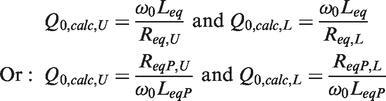
Signal-to-noise ratio (SNR) comparisons performed on: (a), (b), (c) a saline phantom and (d), (e), (f) in vivo on rabbit dermis. The SNR was measured along a 30 mm long line orthogonal to the surface (dashed lines on the magnetic resonance images). The measurements with the dedicated surface coil are represented by the images in (a) and (d) and are plotted in (c) and (f) as the continuous upper curve. The measurements with the volume knee coil were performed on images (b) and (e) and are presented as the lower dashed curves in (c) and (f). The location of the circular-shaped coil is displayed by the small circles right above the surface standing for the cross-section of the loop in (a) and (d).

For MR imaging on the rat, the tail was inserted into the volume coil to image the first caudal vertebrae. The acquisition sequence was a 3D gradient echo sequence with TR = 50 ms, TE = 16 ms, NEX = 1, FA = 20°, matrix = 192 × 192 × 52, FOV = 120 mm × 120 mm ×31.2 mm (voxel volume of 0.625 × 0.625 × 0.6 mm³), and for an acquisition time of 8 min 19 s. For this sequence, the estimated readout time was about 30 ms, giving a 30–40 Hz/pixel receive bandwidth. This sequence was optimized through flip angle choice to get the best contrast for intervertebral disks. SNR comparison was performed between this volume coil and the surface coil designed for the rabbit study in which the tail was inserted.

Results and discussion

In preclinical imaging on small and medium-sized animals such as rats or lagomorphs, there is no low-field MRI device (B₀ below 0.5 T), apart from 1.0 T and 1.5 T devices that are costly and are usually considered to be low-field preclinical MRI devices. Clinical whole body systems, which are not always available for research and preclinical purposes, are even more costly. The use of a low-field (0.18 T) clinical MRI device dedicated to veterinary and preclinical practice with an open magnet sufficiently wide for lagomorphs (∼200 mm) offered an alternative to conventional preclinical MRI and with several advantages. First the initial and maintenance costs of the device are reduced (averaging around €0.35M for a clinical 0.2 T, compared with about €1M for a clinical 1.5 T and nearly €2M for a clinical 3.0 T). The use of a clinical device dedicated to animals has the advantage of avoiding the issues related to hygiene or allergies if regular clinical MRI devices are used with animals. The main advantage of low-field MRI is that, since the sample losses are reduced compared to those of high-field experiments (>0.5 T), the optimization of coils can generate a large increase in SNR. The use of optimized coils with medium-sized or small animals permits the generation of high spatial resolution images within an acceptable acquisition time. Low-field MRI is therefore well adapted for many preclinical studies. Moreover, the high cost of commercially supplied coils may encourage the design and conception of home-made dedicated coils. However the limitations of low-field systems are the low SNR which results if receive coils are not optimized, and an inability to perform studies such as spectroscopy.

For both studies performed on the clinical 0.18 T MRI device, the measured and calculated values of the actual quality factors Q₀ for the surface and volume coils are reported in Table 1.

Table 1.

Measured and calculated values of the actual quality factor Q₀ for the surface and volume coils when unloaded (Q₀ _,U ) and loaded (Q₀ _,L ) with a 0.45% saline solution.

	Q ₀ _,U		Q ₀ _,L		Q₀ _,U /Q₀ _,L
Coil	Measured	Calculated	Measured	Calculated	Measured	Calculated
Surface	98 ± 1	102 ± 1	98 ± 1	98 ± 1	∼1.00	∼1.04
Volume	199 ± 1	198 ± 1	199 ± 1	191 ± 1	∼1.00	∼1.04

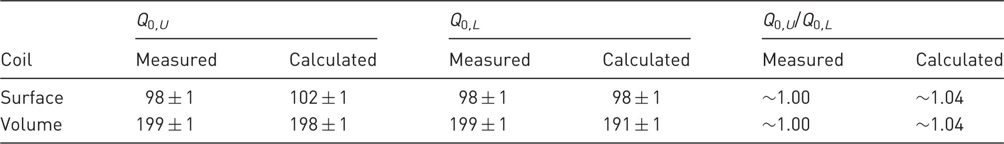
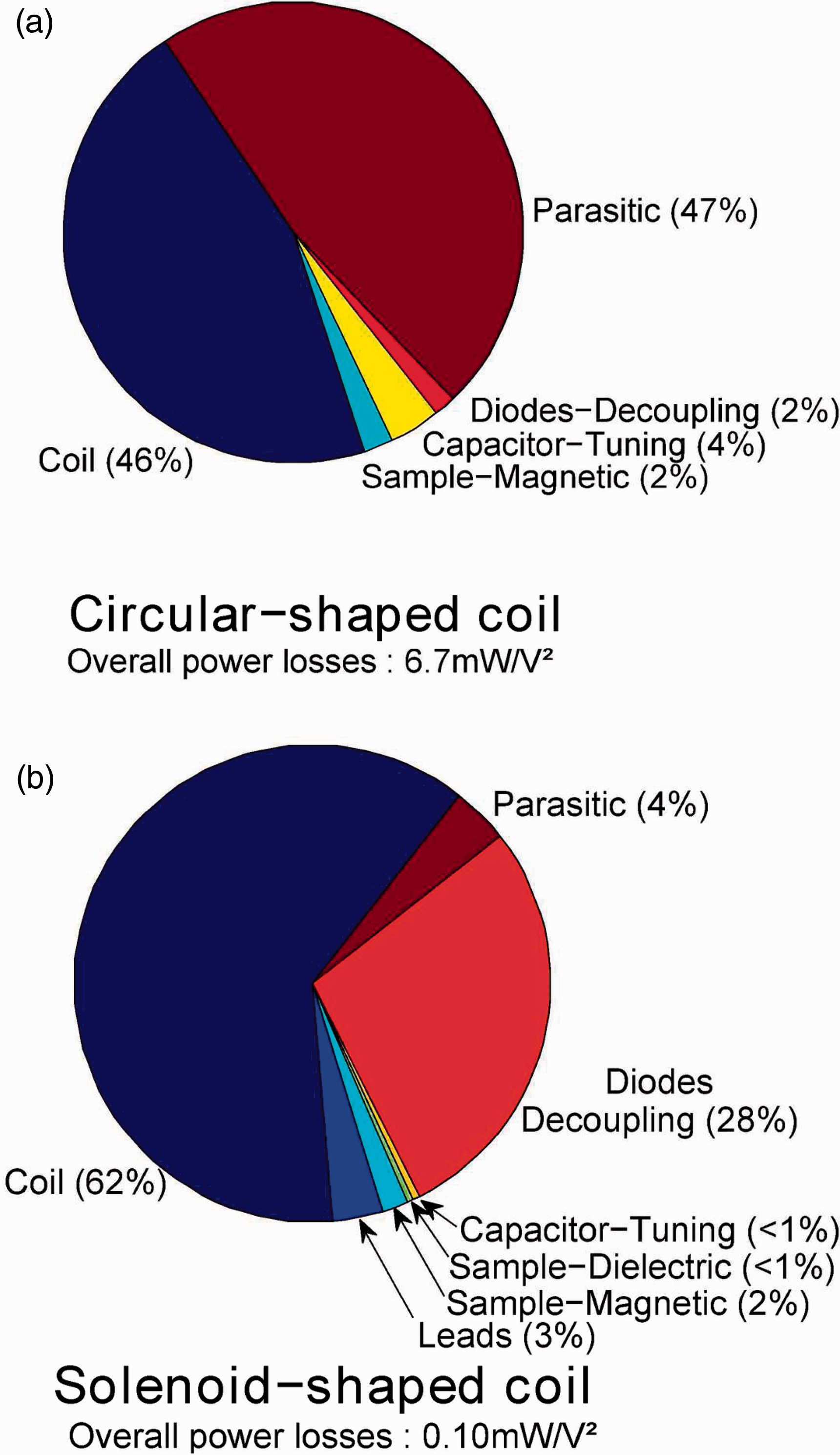
Measured or calculated Q₀ _, _U /Q₀ _, _L ratios were close to unity for the two coils. In other words, sample losses are negligible compared to coil losses. This was to be expected, given the small size of the coils.^15,16 The advantage of such an outcome is that the coils remain matched to Z₀ when samples with electrical characteristics close to biological tissue are inserted. The comparison between measured and calculated Q₀ factors for both coils showed a discrepancy of less than 5% both when they were and were not loaded with a phantom, which validated the model. According to these simulations, the parasitic losses in the two coils did not account for more than 7 mΩ in series with the loop. Yet, this would represent 47% of the over all losses in the surface coil (see Appendix A, Figure 10a). Accurate simulation of such small coils is therefore crucial as the SNR is dependent on small loss phenomena. The quality factors of both coils would have been slightly increased using a thicker copper wire, or using wire with a rectangular cross-section. An analytical model for this kind of wire in a loop coil was notably proposed by Li et al.³⁵ However wires with a rectangular section are usually more difficult to purchase.

In the MRI experiments on rabbits for the intradermal gel study, a comparison between the designed surface coil (10 mm radius) and the commercial knee coil (∼100 mm radius) is presented in Figures 7a to 7c and 7d to 7f, respectively.

At point {x, y, z} = {0, 0, z₀}, with z₀ = 2 mm the distance from surface coil center to skin (or phantom) surface, the ratio between the SNR of the surface coil and the mean SNR inside the commercial knee volume coil was around 14 both on the phantoms (Figure 7c) and in vivo (Figure 7f). For the volume quantification, it was essential that the volume of the voxels was minimized (0.51 × 0.51 × 0.6 mm³ was the minimum accessible with the gradients of the MRI device employed here) to reduce volume quantification error. It was also important that the total acquisition time remained short to minimize anesthetic hazard and improve rabbit recovery. A scan time of 12 min 41 s for each injection site was considered a good compromise to allow the acquisition of images with a sufficient SNR (∼80) using the surface coil. Based on these considerations, both with regard to spatial resolution and SNR, the study would not have been feasible using the commercial coils at our disposal (mean SNR ∼ 8, see Figure 7e), or it would have required a scan duration 100 times longer.

The in vitro validation study gave for the 100 µL tubes a repeatability of 4.7% and an accuracy of 0.5%. The MR acquisition protocol associated with the dedicated surface coil was therefore appropriate for the rabbit study with volumes ranging from 130 µL to 420 µL.

The results of the in vivo volume measurements are summarized in Figure 8. Significant increases (P value <0.1) in the volumes of the four gels were measured from d0 to d28, as well as from d0 to d84. However, no conclusions could be drawn, according to the statistical tests, concerning differences in volume increases between any of the four gels.

Figure 8.

In vivo volume measurements at day 0 (d0, blue), day 28 (d28, red) and day 84 (d84, green) of the four gels injected in the rabbit dermis (n = 5 rabbits). A significant swelling (P < 0.1) was measured from d0 to d28, and also from d0 to d84. See online version for all colour references.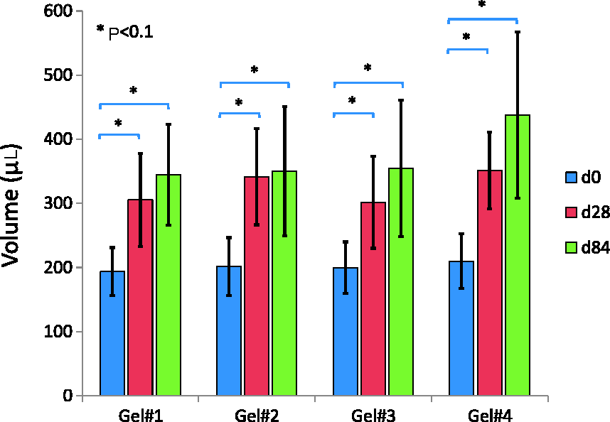

MR images performed on microtubes (for the validation study), on phantoms (for comparison with the commercial coil), and on rabbits showed that the SNR provided by the surface coil with the 3D sequence was suitable for quantifying the volume of injected gels, making it possible to follow volume variations in the gels. Yet, some injection sites had issues – for example some of them leaked or failed, some injections were subcutaneous instead of intradermal, and some even leaked outside the body. The volume of these sites (20 out of 40) was therefore not measurable. Statistical results over the 20 measurable volumes showed that all four gels swelled by 85% with a standard deviation of 24% between d0 (initial volume 200 µL) and d84. This high standard deviation was due to the small number of measurable volumes (5 per gel) and the locations of the injection sites which varied from one animal to another, probably inducing variability in the response of the bodies. The intradermal injections also changed in shape or size across the study, which was to be expected.⁹ Nevertheless, the ROI was still included in the FOV of the coil, as presented in Figure 6d, and the volume quantification was still possible. When designing the surface coil, a radius security margin could have been an option (by increasing the radius by 20%, for example), but that would be at the expense of a decrease in coil sensitivity. For this study, we chose to maximize the SNR at a depth of 10 mm into the rabbit and reduce the radius of the coil at its minimum, i.e. 10 mm.

Concerning the volume coil dedicated to the rat tail, the model confirmed that for solenoid-shaped coils of this size, coil losses are still dominant.^28,21,26 Reducing the radius R to its minimum for this specific rat breed would ultimately maximize SNR, but the available margin (1.5 mm on both sides for the largest tails) was found to be practical for the experimental set-up. Sequence parameters were chosen to provide a good SNR (= 126 ± 1) on intervertebral disks (Figures 9a and 9b) along with a good spatial resolution (0.625 mm/pixel in-plane and 0.6 mm of slice thickness). In comparison, the SNR obtained with the rat tail in the surface coil was 109 ± 1 over the same ROI (Figures 9c and 9d).

Figure 9.

Rat tail images for the in vivo examination of intervertebral structures with (a) the volume coil and (c) the single turn surface coil both in sagittal view. As a result of 3D acquisition, the same images were also observable in transverse view when cutting on the dashed line, as illustrated in (b) and (d) for volume and surface coil, respectively (ImageJ Volume Viewer). The transverse view is obtained without significant loss in image resolution as a result of the quasi-isotropic acquisition. The scale is identical for all four images.

Figure 10.

Proportions of the various losses in: (a) the circular loop coil; (b) the solenoid-shaped coil.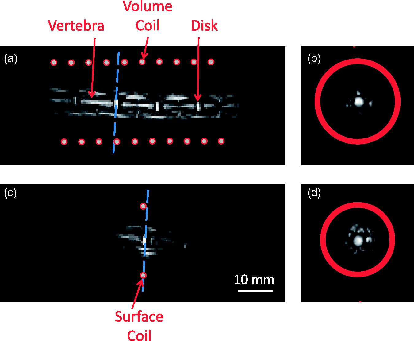

Given the definition of a volume coil, the latter was preferred to the single loop surface coil since B_1xz variations are significantly smaller, which made it more suitable for this application. Moreover, it was particularly valuable to easily localize a specific disk and to be able to observe five of them at a time.^10,12 The intervertebral disks of these rats was measured at approximately 25 ± 2 µL (the voxel volume being about 0.23 µL), which was in accordance with literature.³⁶

Conclusion

Clinical low-field MRI has great potential, especially for those longitudinal preclinical studies which otherwise usually require a large number of animals to be euthanized over time. Indeed, clinical MRI allows the use of a reduced number of animals in non-invasive longitudinal studies of medium-sized and small animal models. In this work, analytical SNR models for coil designs have revealed the importance of small coil optimization for low-field MRI, since sample losses become negligible. Using these easily built home-made coils at 0.18 T, the images in both studies described here had an SNR (>100) suitable for the accurate measurement of small volumes, with a satisfactory image acquisition time of about 10 min. Accurate quantification of small volumes varying from 200 µL down to 25 µL is thus possible with low-field MRI. The design procedure proposed in this paper is clearly applicable to other low-field strengths, such as at 0.4 T, where the SNR is intrinsically better.

Footnotes

Acknowledgements

This work has been funded by the French National Association for Research and Technology (ANRT) and the French Ministry of Higher Education and Research, and was performed within the MRI Center for Animals (CIRMA). This work was also performed within the framework of the LABEX PRIMES (ANR-11-LABX-0063) of Université de Lyon, within the program ‘Investissements d’Avenir’ (ANR-11-IDEX-0007) operated by the French National Research Agency (ANR).

Appendix A: Loss contributions in a low-field MRI coil

References

Breton

Goetz

Choquet

Constantinesco

. Low field magnetic resonance imaging in rat in vivo. IRBM 2008; 29: 366–374.

Wolf

Lam

Mooyaart

Bleichrodt

Nieuwenhuis

Schakenraad

. Magnetic resonance imaging using a clinical whole body system: an introduction to a useful technique in small animal experiments. Lab Anim 1992; 26: 222–227.

Beuf

Jaillon

Saint-Jalmes

. Small-animal MRI: signal-to-noise ratio comparison at 7 and 1.5 T with multiple-animal acquisition strategies. Magn Reson Mater Phys Biol Med 2006; 19: 202–208.

Blasiak

Volotovskyy

Deng

Foniok

Tomanek

. A comparison of MR imaging of a mouse model of glioma at 0.2 T and 9.4 T. J Neurosci Methods 2012; 204: 118–123.

Sasaki

Miyazaki

Takahashi

. Hylan G-F 20 induces delayed foreign body inflammation in guinea pigs and rabbits. Toxicol Pathol 2003; 31: 321–325.

Alessandrini

Di Bartolo

Pavesio

Pressato

. ACP gel: a new hyaluronic acid-based injectable for facial rejuvenation. Preclinical data in a rabbit model. Plast Reconstr Surg 2006; 118: 341–346.

Mandava

Ravuri

Konathan

. High-resolution ultrasound imaging of cutaneous lesions. Indian J Radiol Imaging 2013; 23: 269–277.

Micheels P, Besse S, Flynn TC, Sarazin D and Elbaz Y. Superficial dermal injection of hyaluronic acid soft tissue fillers: comparative ultrasound study. Dermatol Surg 2012; 38(7 Pt 2): 1162–1169.

Gensanne

Josse

Schmitt

Lagarde

Vincensini

. In vivo visualization of hyaluronic acid injection by high spatial resolution T2 parametric magnetic resonance images. Skin Res Technol 2007; 13: 385–389.

10.

Issy

Castania

. Experimental model of intervertebral disc degeneration by needle puncture in Wistar rats. Braz J Med Biol Res 2013; 46: 235–244.

11.

Zhang

La Marca

Hollister

Goldstein

Lin

C-Y

. Developing consistently reproducible intervertebral disc degeneration at rat caudal spine by using needle puncture. J Neurosurg Spine 2009; 10: 522–530.

12.

Keorochana

Johnson

Taghavi

. The effect of needle size inducing degeneration in the rat caudal disc: evaluation using radiograph, magnetic resonance imaging, histology, and immunohistochemistry. Spine J 2010; 10: 1014–1023.

13.

Doty

Entzminger

Kulkarni

Pamarthy

Staab

. Radio frequency coil technology for small-animal MRI. NMR Biomed 2007; 20: 304–325.

14.

Hayes

Axel

. Noise performance of surface coils for magnetic resonance imaging at 1.5 T. Med Phys 1985; 12: 604–607.

15.

Hoult

Richards

. The signal-to-noise ratio of the nuclear magnetic resonance experiment. J Magn Reson 1976; 213: 329–343.

16.

Hoult

Lauterbur

. The sensitivity of the zeugmatographic experiment involving human samples. J Magn Reson 1979; 34: 425–433.

17.

Ocegueda

Rodríguez

. A simple method to calculate the signal-to-noise ratio of a circular-shaped coil for MRI. Concepts Magn Reson Part A 2006; 28A: 422–429.

18.

Minard

Wind

. Solenoidal microcoil design. Part I: Optimizing RF homogeneity and coil dimensions. Concepts Magn Reson 2001; 13: 128–142.

19.

Knight D. The self-resonance and self-capacitance of solenoid coils [Internet]. g3ynh.info. 2013 [cited 2014 Mar 4]. http://www.g3ynh.info/zdocs/magnetics/appendix/self-res.html.

20.

Minard

Wind

. Solenoidal microcoil design. Part II: Optimizing winding parameters for maximum signal-to-noise performance. Concepts Magn Reson 2001; 13: 190–210.

21.

Doty FD. Probe design and construction. In: Encyclopedia of magnetic resonance. Chichester: John Wiley & Sons, Ltd, 2007.

22.

Gadian

Robinson

. Radiofrequency losses in NMR experiments on electrically conducting samples. J Magn Reson 1979; 34: 449–455.

23.

Gabriel

Lau

Gabriel

. The dielectric properties of biological tissues: II. Measurements in the frequency range 10 Hz to 20 GHz. Phys Med Biol 1996; 41: 2251–2269.

24.

Jiang

. Calculating efficient noise resistance of RF coils in low field MRI systems. PIERS Online 2007; 3: 879–882.

25.

Fujita

. New horizons in MR technology: RF coil designs and trends. Magn Reson Med Sci 2007; 6: 29–42.

26.

Lemdiasov

Obi

Ludwig

. A numerical postprocessing procedure for analyzing radio frequency MRI coils. Concepts Magn Reson Part A 2011; 38A: 133–147.

27.

Blasiak

Volotovskyy

Deng

Tomanek

. An optimized solenoidal head radiofrequency coil for low-field magnetic resonance imaging. Magn Reson Imaging 2009; 27: 1302–1308.

28.

Suits

Garroway

Miller

. Surface and gradiometer coils near a conducting body: the lift-off effect. J Magn Reson 1998; 135: 373–379.

29.

Chen

C-N

Hoult

. Biomedical magnetic resonance technology, Bristol: Adam Hilger, 1989.

30.

Wheeler

Conradi

. Practical exercises for learning to construct NMR/MRI probe circuits. Concepts Magn Reson Part A 2012; 40A: 1–13.

31.

Murphy-Boesch

Koretsky

. An in vivo NMR probe circuit for improved sensitivity. J Magn Reson 1983; 54: 526–532.

32.

Decorps

Blondet

Reutenauer

Albrand

Remy

. An inductively coupled, series-tuned NMR probe. J Magn Reson 1985; 65: 100–109.

33.

Kajfez

Hwan

. Q-factor measurement with network analyzer. IEEE Trans Microw Theory Tech 1984; 32: 666–670.

34.

Edelstein

Bottomley

Pfeifer

. A signal-to-noise calibration procedure for NMR imaging systems. Med Phys 1984; 11: 180–185.

35.

Webb

Saha

Brey

Zachariah

Edison

. Comparison of the performance of round and rectangular wire in small solenoids for high-field NMR. Magn Reson Chem 2006; 44: 255–262.

36.

Iatridis

Mente

Stokes

Aronsson

Alini

. Compression-induced changes in intervertebral disc properties in a rat tail model. Spine 1999; 24: 996–1002.

37.

Medhurst

. H.F. resistance and self-capacitance of single-layer solenoids. Wirel Eng 1947; 24: 35–43, 80–92.

38.

Van Heteren

Henkelman

Bronskill

. Equivalent circuit for coil-patient interactions in magnetic resonance imaging. Magn Reson Imaging 1987; 5: 93–99.

39.

Grandi

Kazimierczuk

Massarini

Reggiani

. Stray capacitances of single-layer solenoid air-core inductors. IEEE Trans Ind Appl 1999; 35: 1162–1168.

Coil optimization for low-field MRI: a dedicated process for small animal preclinical studies

Abstract

Keywords

Materials and methods

Animals

Instruments

Coil optimization

Mathematical model

Coil fabrication

Electrical characterization

MRI

Results and discussion

Conclusion

Footnotes

Acknowledgements

Appendix A: Loss contributions in a low-field MRI coil

References