Correcting Regressor-Endogeneity Bias via Instrument-Free Joint Estimation Using Semiparametric Odds Ratio Models

Abstract

Endogenous regressors can lead to biased estimates for causal effects using methods assuming regressor–error independence. To correct for endogeneity bias, the authors propose a new method that accounts for the regressor–error dependence using flexible semiparametric odds ratio conditional models; the approach requires neither parametric distributional assumptions nor tuning parameters for modeling endogenous regressors’ distributions conditional on the error term and exogenous regressors. Inference is achieved via optimizing the profile likelihood concentrating on the parameters of interest. The proposed approach requires no use of instrumental variables (IVs), observed or latent, that must satisfy the stringent condition of exclusion restriction. Nonnormally distributed endogenous regressors are required for model identification with a normal error distribution. The approach's flexibility in capturing regressor–error dependence increases the capability of IV-free endogeneity correction and provides opportunities to improve the accuracy of causal effect estimation. Unlike existing IV-free methods, the proposed approach can handle discrete endogenous regressors with few levels, such as binary regressors or count regressors with small means, and is thus applicable to a plethora of applications involving such regressors. The authors demonstrate the versatility of the approach for binary, count, and continuous endogenous regressors using comprehensive simulation studies and empirical data.

In many empirical marketing studies, researchers need to control for regressor endogeneity when estimating population structural regression models representing causal relationships of interest. We refer to regressor endogeneity as whenever a regressor relates to the regression error term, causing regressor–error dependence. By contrast, an exogenous regressor is predetermined or controlled by researchers such that units are randomly assigned to different regressor values, rendering the regressor and the error term independent. Because many data are observational in nature, regressors are frequently not randomly assigned. In almost all of these applications, the assumption that all regressors are exogenous is debatable, if not untenable. For example, the error term (henceforth “structural error”) in a consumer demand model may include unobserved common market shocks or product attributes affecting marketing-mix regressors (e.g., price) (Villas-Boas and Winer 1999).

Endogeneity can greatly hinder unambiguous conclusions regarding causal effects. Estimation methods assuming all regressors are exogenous, such as ordinary least squares (OLS), can yield severely biased causal effect estimates when regressors are actually endogenous. The instrumental variable (IV) approach is traditionally used to correct for endogeneity bias but requires valid and strong IVs, which can be hard to find and validate in practice (Rossi, Allenby, and McCulloch 2005). Recent marketing literature also emphasizes the need for more flexible ways to handle regressor endogeneity (Dost et al. 2019; Zhang, Kumar, and Cosguner 2017).

This work aims to develop an IV-free joint estimation approach to correcting for endogeneity bias based on semiparametric odds ratio endogeneity (SORE) models. SORE addresses endogeneity bias by accounting for regressor–error dependence via joint modeling of these random variables. Specifically, we model the distribution of endogenous regressors conditional on the structural error and exogenous regressors using the semiparametric odds ratio (SOR) models (Chen 2004; Feit and Bradlow 2021; Qian and Xie 2011, 2014, 2015, 2022). Under SORE, this conditional distribution comprises two components: (1) the flexible odds ratio (OR) functions capturing the regressor–error dependence and describing the nature and magnitude of endogeneity unexplained by the exogenous control variables, and (2) nonparametric baseline distribution functions capturing the distributional features of endogenous regressors critical for proper correction of endogeneity bias. The likelihood function based on the joint distribution of the error term and endogenous regressors given exogenous ones is then derived and optimized to obtain the maximum likelihood estimation (MLE) of model parameters. We derive sources of identification for a range of OR functions encoding different identification strategies and demonstrate how to select appropriate ones empirically using likelihood-based model selection measures. SORE is applicable to both discrete (including binary and count) and continuous endogenous regressors without imposing parametric distributional assumptions on them, and permits endogeneity correction to be conditioned on exogenous regressors without imposing models on exogenous regressors.

The main contributions of SORE lie in the following aspects. First, SORE offers a general and flexible regressor-endogeneity bias-correction framework that increases the capability of IV-free endogeneity correction. We show that SORE provides likelihood-based counterparts of some extant IV-free methods, such as identification via heteroskedasticity and higher moments (Lewbel 1997; Rigobon 2003), and nests the recently proposed joint copula modeling (JCM) approach (Becker, Proksch, and Ringle 2021; Eckert and Hohberger 2023; Park and Gupta 2012; Tran and Tsionas 2021) as a special case. To correct for endogeneity bias, JCM assumes a Gaussian copula (GC) model (Danaher and Smith 2011) to capture regressor–error dependence. We show that, theoretically, JCM is a special case of SORE with particular forms of OR functions and baseline distribution functions and thus is fully nested within the SORE framework. By considering OR functions permitting both copula and noncopula dependence, SORE builds on the wide applicability of JCM and its recent extensions (Haschka 2022; Yang, Qian, and Xie 2022) and addresses broader types of regressor endogeneity, providing novel ways to identify causal effects.

Second, SORE provides a novel IV-free approach for handling discrete endogenous regressors that overcomes the limitations of existing IV-free methods. Among existing IV-free methods, only JCM can handle discrete endogenous regressors (Park and Gupta 2012). JCM views discrete endogenous regressors as realizations from underlying continuous latent variables and performs an inverse mapping from the cumulative distribution functions (CDFs) of endogenous regressors to the latent variables. One limitation of the approach and its recent extensions (Haschka 2022; Yang, Qian, and Xie 2022) is that endogenous regressors must contain adequate information, in that the number of unique values for these regressors cannot be too small (Eckert and Hohberger 2023; Haschka 2022; Park and Gupta 2012; Tran and Tsionas 2021; Yang, Qian, and Xie 2022). A plethora of applications involve discrete endogenous regressors that take on a small set of possible values. Examples include binary variables for coupon promotion and count variables with small means (e.g., the number of coupons redeemed by a consumer for durable goods). Theoretical challenges and empirical identification issues for nonparametric copula estimation due to plateaus in the inverse of empirical discrete CDFs have been documented in the literature (Genest and Nešlehová 2007). Unlike JCM, SORE provides specifications requiring no inverse mapping from the CDFs of endogenous regressors, thus avoiding the nonuniqueness of this mapping and the consequent model nonidentifiability issue for discrete endogenous regressors that JCM and its recent extensions encounter. Under SORE, handling discrete endogenous regressors is straightforward with simple-to-evaluate likelihood involving no latent variables.

Third, SORE offers certain estimation/inferential advantages over two-step IV-free methods. Unlike the two-step JCM procedures, SORE estimates model parameters in one step and has several important advantages shared by the recently proposed one-step JCM (Tran and Tsionas 2021), including greater estimation efficiency (smaller estimate variability) and improved capability to detect endogeneity by using all data simultaneously, availability of maximized likelihood for likelihood-based model comparisons, and direct estimation of standard errors without resorting to bootstrap resampling.

These benefits of SORE are not without costs. Misspecifying OR functions can introduce bias into endogeneity correction or cause model nonidentification. Although SORE allows for flexible modeling of dependence structures, we only consider OR functions built from two broad types of dependence structures, GC and log-bilinear (LB), that have proven identifiability and encompass a number of existing dependence models. Because model nonidentification causes singular Hessian matrices of the likelihood functions and huge standard error estimates, it is important to check the sizes of standard errors to detect potential OR misspecifications. Although model comparison can help select proper OR functions, model selection methods are not error-free and involve a trade-off between estimation bias and variance. For instance, the GC regressor–error dependence assumed in JCM is a flexible and robust model applicable in many marketing applications to capture relationships among variables (Danaher and Smith 2011; Eckert and Hohberger 2023). SORE provides OR specifications that generalize JCM to permit flexible forms of regressor–regressor dependence. However, if endogenous and exogenous regressors are indeed independent, JCM will outperform SORE because a simpler and correct model outperforms more general models. In general, estimation after selection from OR functions will underperform as compared with the case with an OR correctly chosen a priori based on substantive knowledge.

SORE can encounter identification issues. With a normal structural error distribution, nonnormally distributed endogenous regressors are required for model identification. When endogenous regressors are normally distributed, SORE estimates are biased toward OLS estimates with hugely inflated standard errors relative to OLS ones. Like IV and other IV-free methods, SORE is a large-sample procedure. Even if a SORE model is theoretically identified with infinite sample size, SORE may encounter weak empirical identification with nearly flat likelihood in a small sample. Such weakly identified models yield almost singular Hessian matrices and very large standard errors. Thus, it is important to check the sizes of standard errors to detect potential lack of empirical identification. The nonparametric baseline functions for continuous endogenous regressors can involve numerous parameters. To make the one-step estimation scalable to large problems, SORE employs a profile likelihood approach that eliminates these nuisance parameters altogether from the model estimation/inference. Still, the two-step JCM that adds generated regressors to control endogeneity requires no such special algorithm and is straightforward to implement with considerably less computation time for continuous endogenous regressors.

In the next section, we review the literature on methods for handling regressor endogeneity. We then describe the proposed methodology, followed by evaluations using simulated data and an illustration in a real data set. The article ends with a discussion.

Literature Review

As regressor endogeneity is such a prevalent and thorny hindrance to causal inference in observational studies, extensive work in economics, statistics, marketing, and other fields has explored remedies to mitigate this issue. Imbens (2020) reviewed the Rubin causal model using potential outcomes and the directed acyclic graphs with “do-calculus” (Pearl and Mackenzie 2018) for analyzing causal effects. The two frameworks are complementary with different strengths, but the Rubin causal model is considered to have closer connections to the causal models used in empirical economics and marketing research (Imbens 2020). In both frameworks, regressor exogeneity (or the closely related unconfoundedness/ignorability) is central in identifying causal effects for a host of methods, including regression adjustment, matching, and weighting (Imbens 2020; Robins, Hernan, and Brumback 2000). Relaxing the key assumption requires additional data or alternative assumptions. Our review focuses on causal inference methods that do not require regressor exogeneity. ¹

IV Methods

As the classical approach to solving the issue of endogeneity bias (Li and Ansari 2014; Rossi, Allenby, and McCulloch 2005), the IV method replaces the assumption of regressor exogeneity with two alternative conditions for IVs: relevance and exclusion restriction. Weak IVs that lack sufficient correlation with endogenous regressors can cause estimation bias to a greater extent than the endogeneity bias. The untestable condition of exclusion restriction requires that IVs be uncorrelated with the error term and affect the outcome only through endogenous regressors. These two conditions are often in conflict, making it challenging to find and validate satisfactory IVs.

Structural Modeling

An alternative way to solve endogeneity bias is to augment the model of interest with a highly structured secondary model describing the exact data generating process for endogenous regressors based on economic theory (Chintagunta et al. 2006). However, theory rarely is detailed enough to prescribe all aspects of the data generating process. Furthermore, identifying structural models often relies on IVs (Chintagunta et al. 2006).

IV-Free Methods Using Generated or Latent IVs

Given the challenges in identifying satisfactory IVs or correctly specifying structural models, interest in developing IV-free econometric methods to address endogeneity issues is growing. These IV-free methods entail neither observing IVs nor specifying a correct structural model of endogenous regressors. Lewbel (1997) shows how to generate IVs based solely on the higher moments (HM) of regression data in the outcome model to correct for endogeneity bias due to error in regressors. Rigobon (2003) proposes an “identification through heteroskedasticity” (IH) procedure that exploits the heteroskedastic error structure to identify structural parameters. Despite requiring no IVs, the IH procedure does require the availability of a grouping variable across which the structural shocks are heteroskedastic.

Ebbes et al. (2005) propose the latent IV method that models an endogenous regressor as a sum of an exogenous component and an endogenous component. The latent IV method then assumes that the exogenous component is a function of a latent discrete exogenous variable. Ebbes, Wedel, and Böckenholt (2009) provide a detailed review of the three preceding IV-free methods. Wang and Blei (2019) propose a “deconfounder” approach to generating IVs using a latent factor model for multiple endogenous causes. Assuming no unobserved single-cause confounders, ² the difference between an endogenous regressor and the estimated latent factor (also called a substitute confounder) is an IV for the regressor.

IV-Free Joint Estimation Methods

The preceding IV-free methods (HM, IH, latent IV, deconfounder) all decompose an endogenous regressor into exogenous and endogenous parts, and employ a critical assumption that the exogenous part includes generated or latent variables satisfying exclusion restriction or the related condition of exogeneity, which can be difficult to justify (Park and Gupta 2012).

An appealing alternative is to directly model regressor–error dependence using a copula without decomposing the endogenous regressors to exogenous and endogenous parts (Park and Gupta 2012). No condition of exclusion restriction or exogeneity is needed in JCM, which significantly increases the feasibility of correcting for endogeneity bias. Meanwhile, recent work also reveals boundary conditions of JCM. Becker, Proksch, and Ringle (2021) and Eckert and Hohberger (2023) show that JCM can yield biased estimates when GC misspecifies regressor–error dependence. Haschka (2022) shows that JCM implicitly assumes independence between endogenous and exogenous regressors and can yield significant bias when they are actually related. Haschka proposes a GC model on the error term and all regressors while extending JCM to panel data analysis. Becker, Proksch, and Ringle show that the two-step JCM can have substantial finite-sample bias and loss of power to detect endogeneity when the structural model includes the intercept term. To overcome some of the estimation drawbacks of the two-step JCM, Tran and Tsionas (2021) develop an efficient sieve estimation of JCM that maximizes the likelihood in one step and requires no bootstrap to obtain standard errors. Their approach uses sieve basis functions to approximate the unknown smooth marginal densities of continuous endogenous regressors, and its performance depends critically on the correct choices of the number of basis functions (i.e., the tuning parameter). They find that one-step estimation reduces standard errors of model estimates and improves the ability to detect endogeneity.

Like JCM and its extensions, SORE requires neither the exclusion restriction nor the exogeneity assumption imposed in other IV-free methods. While nesting JCM and all its recent extensions as special cases, SORE is not restricted to copula dependence, permits noncopula types of regressor–error and regressor–regressor dependence, and can handle binary endogenous regressors and count endogenous regressors with small means (Table 1). The one-step SORE estimation is not subject to the finite-sample bias issue in models with an intercept affecting the two-step JCM (Becker, Proksch, and Ringle 2021). Meanwhile, unlike the one-step estimation approach of Tran and Tsionas (2021), SORE requires no tuning parameters when modeling endogenous regressors nonparametrically and imposes no assumption of smooth marginal densities for endogenous regressors.

Table 1.

Comparison of SORE with Existing IV-Free Joint Estimation Methods.

	Park and Gupta (2012), Becker, Proksch, and Ringle (2021), Eckert and Hohberger (2023)	Tran and Tsionas (2021)	Haschka (2022)	SORE
Regressor–error dependence	GC	GC	GC	Includes GC as a special case and permits noncopula dependence
Regressor–regressor dependence	Assume independence	Assume independence	GC	Can handle both GC and flexible noncopula dependence
Handle discrete endogenous regressors with few levels	No	No	No	Yes
Estimation method	Two-step	One-step	Two-step	One-step
	Require tuning parameter in MLE			No tuning parameter

Notes: Tuning parameter refers to the bandwidth in the kernel estimator (Haschka 2022; Park and Gupta 2012) or the number of sieve basis functions (Tran and Tsionas 2021) used to model regressors’ marginal density functions.

Multivariate Modeling

SORE models the multivariate distribution of endogenous regressors and the structural error conditional on exogenous regressors, using the SOR model that we review here. Flexible multivariate models are sought in many fields (Danaher and Smith 2011). One example is the Sarmanov distribution, which combines disparate parametric marginals (e.g., exponential-gamma models for continuous variables, negative binomial models for discrete variables) into a multivariate distribution (Danaher 2007; Park and Fader 2004). Its limitations include that it does not scale well to many random variables, and the range of the correlation parameter capturing dependence can be less than the full range of (−1, 1). This is where the GC model has considerable advantage, as shown in the influential work of Danaher and Smith (2011). Park and Gupta (2012) used the GC model with nonparametric marginals for endogenous regressors. The SORE model nests both Sarmanov and GC as special cases, in that the latter two can be expressed as SORE models with particular forms of OR functions and baseline functions. Furthermore, only SORE simultaneously possesses all three of the following capabilities, crucial for addressing regressor-endogeneity bias: (1) it combines disparate univariate distributions into a multivariate distribution without imposing parametric distributional assumptions on endogenous regressors, (2) it provides flexibility in modeling various forms of dependence, and (3) it permits the multivariate distribution to be conditional on exogenous regressors.

Despite being a much more recent newcomer, SOR has demonstrated its power in modeling multivariate distributions (Chen 2004, 2007). Qian and Xie (2011) develop a new Bayesian method to address partially observed covariates in marketing models, which avoids evaluating the high-dimensional likelihood associated with multiple partially observed covariates and reduces the increase in computational workload from an exponential rate to a linear rate. SOR models have also been employed for robust and flexible data fusion (Feit and Bradlow 2021; Qian and Xie 2014) and secure business analytics preserving data privacy (Qian and Xie 2015). Qian and Xie (2022) adapt SOR models to simplify analyses of informative samples collected via endogenous selective sampling, which draws sampling units based on the outcome values to enrich sample information. However, none of these methods is designed to handle regressor-endogeneity bias. ³ Furthermore, we propose using the profile likelihood, which eliminates all the nuisance parameters in baseline functions from model inference. Finally, we demonstrate for the first time that SOR nests the commonly used copula models as special cases.

Methodology

The SORE Approach to Correcting for Endogeneity Bias

To illustrate the approach, we first consider the structural linear regression model

$$\begin{array}{c}{\mathrm{Y}}_{\mathrm{i}}=\mu +{\mathrm{X}}_{\mathrm{i}}^{\mathrm{T}}\alpha +{\mathrm{W}}_{\mathrm{i}}^{\mathrm{T}}\beta +{\mathrm{E}}_{\mathrm{i}},\end{array}$$

(1)

where ${\mathrm{W}}_{\mathrm{i}}^{\mathrm{T}}$  = (W_i1, …, W_iQ) contains Q exogenous regressors independent of the structural error E_i; ${\mathrm{X}}_{\mathrm{i}}^{\mathrm{T}}$ = (X_i1, …, X_iK) contains K endogenous regressors, each associated with E_i; and i = 1, …, n indexes independent units. Both W and X can contain a mixture of continuous and discrete variables. Throughout, we make the following structural model assumptions:

• 1. ${\mathrm{E}}_{\mathrm{i}}\stackrel{\mathrm{i}.\mathrm{i}.\mathrm{d}.}{\sim }{\mathrm{f}}_{\varphi }(\cdot )$ .

• 2. $\mathbb{E}[{(1,{\mathrm{X}}_{\mathrm{i}}^{\mathrm{T}},{\mathrm{W}}_{\mathrm{i}}^{\mathrm{T}})}^{\mathrm{T}}(1,{\mathrm{X}}_{\mathrm{i}}^{\mathrm{T}},{\mathrm{W}}_{\mathrm{i}}^{\mathrm{T}})]$ has full rank of 1 + K + Q.

• 3. ${\mathrm{W}}_{\mathrm{i}}\mathrm{\perp }{\mathrm{E}}_{\mathrm{i}}$ but E_i can be associated with X_i.

Assumption 1 states that E_i, i = 1, …, n, are i.i.d. with the marginal probability density function (PDF), f_ϕ(E_i), indexed by the parameter ϕ. A common choice for f_ϕ(E_i) is a normal density (0, σ²) (e.g., Ebbes et al. 2005; Park and Gupta 2012; Villas-Boas and Winer 1999). No restriction is imposed on the conditional distribution of the error term given regressors: E_i | X_i, W_i. The parameter of interest is θ = (α, β, μ, ϕ). Assumption 2 means no perfect collinearity among regressors. Unlike the exogenous regressors in W, whose distributions are ancillary to the parameter of interest θ, the distributions of the endogenous regressors in X provide information about θ via their associations with the structural error term under Assumption 3. Thus, the single-equation OLS estimation of Equation 1 ignoring these associations can lead to significant estimation bias, which can be viewed as a model misspecification bias because OLS incorrectly assumes Cov(X_i, E_i) = 0.

The SORE approach to handling endogeneity does not require additional data or the use of (observed or latent) IVs, but directly estimates the joint distribution of (E_i, X_i) given W_i. To simplify the exposition, subsequently we suppress the index i and consider the case of X containing one regressor. The next subsection will consider multiple regressors in X. Our approach expresses the joint distribution of (E, X) | W as ⁴

$$\begin{array}{c}\mathrm{f}(\mathrm{E},\mathrm{X}|\mathrm{W})={\mathrm{f}}_{\varphi }(\mathrm{E}|\mathrm{W}){\mathrm{f}}_{\psi }(\mathrm{X}|\mathrm{E},\mathrm{W})={\mathrm{f}}_{\varphi }(\mathrm{E}){\mathrm{f}}_{\psi }(\mathrm{X}|\mathrm{E},\mathrm{W}),\end{array}$$

(2)

where f_ϕ(E | W) = f_ϕ(E) as W is exogenous, and f_ψ(X | E, W) is a PDF when X is continuous or a probability mass function when X is discrete. We consider the preceding modeling approach natural to model regressor endogeneity. For example, f_ψ(X | E, W) can capture the dependence of X on omitted variables that become elements in E, or on E directly due to reverse causality or simultaneity. ⁵

Although f_ψ(X | E, W) is typically not of interest, a correctly specified model for f_ψ(X | E, W) is important because misspecifying this nuisance distribution can introduce bias into the estimation of the parameter of primary interest, θ. In practice, correctly modeling f_ψ(X | E, W) is challenging because (1) X can contain a mixture of continuous, discrete, or semicontinuous regressors; (2) X can exhibit complex distributional features, such as boundedness, discreteness, multimodality, skewness, and heavy tails, which are critical for model identification and so must be faithfully preserved in modeling; and (3) there exist various forms of regressor–error and regressor–regressor dependence structure. Standard parametric distributional forms for f_ψ(X | E, W) may fail to maintain important distributional features of endogenous regressors critical for model estimation, or even fail to achieve model identification (see the “Model Identification” section). For these reasons, we chose to model f_ψ(X | E, W) using a SOR model (Chen 2004; Qian and Xie 2011) as

$$\begin{array}{ccc}{\mathrm{f}}_{\psi }(\mathrm{X}=\mathrm{x}|\mathrm{E}=\mathrm{e},\mathrm{W}=\mathrm{w})& ={\displaystyle \frac{{\eta }_{\gamma }(\mathrm{x},{\mathrm{x}}_0;\mathrm{e},{\mathrm{e}}_0,\mathrm{w},{\mathrm{w}}_0){\mathrm{f}}_{\lambda }(\mathrm{x}|{\mathrm{e}}_0,{\mathrm{w}}_0)}{\int {\eta }_{\gamma }(\mathrm{x},{\mathrm{x}}_0;\mathrm{e},{\mathrm{e}}_0,\mathrm{w},{\mathrm{w}}_0){\mathrm{f}}_{\lambda }(\mathrm{x}|{\mathrm{e}}_0,{\mathrm{w}}_0)\mathrm{dx}},}& \end{array}$$

(3)

where f_ψ(x | e, w) is decomposed as a function of two components: (1) the OR function,

$$\begin{array}{cc}{\eta }_{\gamma }(\mathrm{x},{\mathrm{x}}_0;\mathrm{e},{\mathrm{e}}_0,\mathrm{w},{\mathrm{w}}_0)={\displaystyle \frac{{\mathrm{f}}_{\psi }(\mathrm{x}|\mathrm{e},\mathrm{w}){\mathrm{f}}_{\lambda }({\mathrm{x}}_0|{\mathrm{e}}_0,{\mathrm{w}}_0)}{{\mathrm{f}}_{\psi }({\mathrm{x}}_0|\mathrm{e},\mathrm{w}){\mathrm{f}}_{\lambda }(\mathrm{x}|{\mathrm{e}}_0,{\mathrm{w}}_0)},}& \end{array}$$

(4)

which captures the associations between X and (E, W) with (x₀, e₀, w₀) being a fixed reference point in the sample space of (X, E, W), and (2) the baseline function, f_λ(x | e₀, w₀), which is the PDF or probability mass function for X at the fixed point (e₀, w₀) and behaves like a marginal distribution. The OR function η_γ(x, x₀; e, e₀, w, w₀) is the ratio of the odds of observing x relative to observing x₀ when (E, W) varies from (e₀, w₀) to (e, w). The reference point (x₀, e₀, w₀) can be chosen arbitrarily, but a value of (x₀, e₀, w₀) remote from the observed data points may lead to numerical overflow in model estimation. For simplicity, we write η(x, x₀; e, e₀, w, w₀) as η(x; e, w) henceforth. Multiplying both sides of Equation 4 by f_ψ(x | e₀, w₀) and then integrating both sides with respect to x leads to Equation 3. One can separately specify the two components as follows and then use Equation 3 to obtain f_ψ(X | E, W).

Nonparametric modeling of the baseline function f_λ(x | e₀, w₀)

To increase modeling robustness and automatically pick up important distributional features of endogenous regressors, we employ the nonparametric empirical modeling approach (Chen 2004) for the baseline function, f_λ(x | e₀, w₀). Specifically, f_λ(x | e₀, w₀) has nonzero probability mass p = (p₁, …, p_L) only on the uniquely observed X values, (u₁, …, u_L), in the data. To relax the constraint $\sum _{l=1}^{\mathrm{L}}{\mathrm{p}}_l=1$ and 0 < p _l  < 1, we reparameterize p as λ = (λ₁, …, λ_L), with λ _l  = ln (p _l  / p_L) and ${\mathrm{p}}_{\mathrm{l}}=\exp ({\lambda }_{\mathrm{l}})/\sum _{l=1}^{\mathrm{L}}\exp ({\lambda }_{\mathrm{l}})$ , for l = 1, …, L. Thus, no parametric distributional assumption is invoked in modeling the baseline distribution function of X.

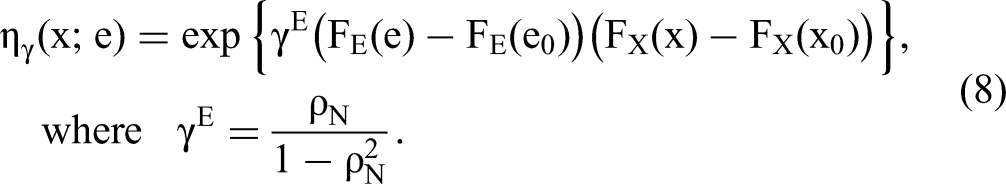
Flexible modeling of the endogeneity via the OR function η_γ(x; e, w)

SORE also excels in modeling various forms of association between (E, W) and X via the OR function, η_γ(x; e, w). When X is a categorical variable, the OR function yields the familiar OR parameters in the multinomial logistic regression of X on E and W. When X is continuous, semicontinuous, or discrete taking infinite possible values (e.g., a count variable), the OR function also exists and can be motivated by relevant parametric counterparts of SORE. Consider that X | (E, W) follows the generalized linear models (GLM) (McCullagh and Nelder 2019):

$${\mathrm{f}}_{\beta ,\tau }(\mathrm{x}|\mathrm{e},\mathrm{w})=\exp \left\{{\displaystyle \frac{\mathrm{x}\mathrm{\Psi }(\beta ,\mathrm{e},\mathrm{w})-\mathrm{b}(\mathrm{\Psi }(\beta ,\mathrm{e},\mathrm{w}))}{\mathrm{a}(\tau )}+\mathrm{c}(\mathrm{x},\tau )}\right\},$$

(5)

where ψ is the canonical parameter and β is a vector mean parameter; b(·) and c(·,·) determine a distribution in the exponential family; and a(τ) = τ / w, with dispersion parameter τ and known weight w. The GLMs include Gaussian, logistic, Poisson, and gamma regressions as special cases. For GLMs with canonical link functions $\mathrm{g}(\mathrm{mean}(\mathrm{x}|\mathrm{e},\mathrm{w}))=$ $\mathrm{\Psi }(\beta ,\mathrm{e},\mathrm{w})={\beta }_0+\sum _{\mathrm{q}=1}^{\mathrm{Q}}{\beta }_{\mathrm{q}}^{\mathrm{W}}{\mathrm{w}}_{\mathrm{q}}+{\beta }^{\mathrm{E}}\mathrm{e}$ , plugging the GLM density functions f(x | e, w), f(x₀ | e₀, w₀), f(x | e₀, w₀), and f(x₀ | e, w) into Equation 4 yields the following log-bilinear (LB) OR function:

$$\begin{array}{c}\ln {\eta }_{\gamma }(\mathrm{x};\mathrm{e},\mathrm{w})=\sum _{\mathrm{q}=1}^{\mathrm{Q}}{\gamma }_{\mathrm{q}}^{\mathrm{W}}({\mathrm{w}}_{\mathrm{q}}-{\mathrm{w}}_{\mathrm{q}0})(\mathrm{x}-{\mathrm{x}}_0)+{\gamma }^{\mathrm{E}}(\mathrm{e}-{\mathrm{e}}_0)(\mathrm{x}-{\mathrm{x}}_0),\end{array}$$

(6)

where the log-OR parameters ${\gamma }_{\mathrm{q}}^{\mathrm{W}}$ and γ^E are reparameterizations of the GLM model parameters: ${\gamma }_{\mathrm{q}}^{\mathrm{W}}=\frac{{\beta }_{\mathrm{q}}^{\mathrm{W}}}{\mathrm{a}(\tau )}$ and ${\gamma }^{\mathrm{E}}=\frac{{\beta }^{\mathrm{E}}}{\mathrm{a}(\tau )}$ . Thus, GLM is a special case of SORE, taking the LB form of the OR function in Equation 6 and a parametric form of the baseline function f_β,τ(x | e₀, w₀), that is, the GLM density function in Equation 5 evaluated at (e₀, w₀).

The OR functions are also closely related to other familiar dependence measures. When (X, E) follows the standard bivariate normal distribution with Pearson's correlation coefficient ρ and marginal variances for X and E being 1, X | E follows a normal linear model, and according to the preceding result for GLMs, X | E has an LB form of OR function: ln η_γ (x; e) = γ^E(x − x₀)(e − e₀) with 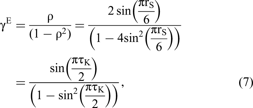${\gamma }^{\mathrm{E}}=\frac{\rho }{1-{\rho }^2}$ . Thus, the log-OR parameter γ^E relates to Pearson's correlation coefficient ρ and two other bivariate dependence measures—Spearman's rank correlation coefficient r_S and Kendall’s τ_K—as

$${\gamma }^{\mathrm{E}}={\displaystyle \frac{\rho }{(1-{\rho }^2)}={\displaystyle \frac{2\sin \left({\displaystyle \frac{\pi {\mathrm{r}}_{\mathrm{S}}}{6}}\right)}{\left(1-4{\sin }^2\left({\displaystyle \frac{\pi {\mathrm{r}}_{\mathrm{S}}}{6}}\right)\right)}={\displaystyle \frac{\sin \left({\displaystyle \frac{\pi {\tau }_{\mathrm{K}}}{2}}\right)}{\left(1-{\sin }^2\left({\displaystyle \frac{\pi {\tau }_{\mathrm{K}}}{2}}\right)\right)},}}}$$

(7)

where $\rho =2\sin \left(\frac{\pi {\mathrm{r}}_{\mathrm{S}}}{6}\right)=\sin \left(\frac{\pi {\tau }_{\mathrm{K}}}{2}\right)$ (Joe 2015, section 2.12.5). When (X, E) does not follow a bivariate normal distribution, the preceding relationship can be extended using dependence measures on normal scores. Define F_E(e) = Φ⁻¹(H_E­(e)) and F_X(x) = Φ⁻¹(H_X(x)) as normal scores of e and x, respectively, where H_E­(·) and H_X­(·) are the CDFs of E and X, respectively; Φ⁻¹(·) is the inverse CDF of the standard normal. Let (F_E(e), F_X(x)) follow a standard bivariate normal distribution with a correlation of ρ_N. Then, one has

$${\eta }_{\gamma }(\mathrm{x};\mathrm{e})=\exp \{{\gamma }^{\mathrm{E}}\left({\mathrm{F}}_{\mathrm{E}}(\mathrm{e})-{\mathrm{F}}_{\mathrm{E}}({\mathrm{e}}_0)\right)\left({\mathrm{F}}_{\mathrm{X}}(\mathrm{x})-{\mathrm{F}}_{\mathrm{X}}({\mathrm{x}}_0)\right)\},\mathrm{where}{\gamma }^{\mathrm{E}}={\displaystyle \frac{{\rho }_{\mathrm{N}}}{1-{\rho }_{\mathrm{N}}^2}.}$$

(8)

More generally, even when X | (E, W) does not follow GLMs, one can interpret parameters in $\gamma =({\gamma }_1^{\mathrm{W}},\dots ,{\gamma }_{\mathrm{Q}}^{\mathrm{W}},{\gamma }^{\mathrm{E}})$ in Equation 6 as odds ratios. From Equations 3 and 6, we have

$$\begin{array}{c}{\displaystyle \frac{{\mathrm{f}}_{\psi }(\mathrm{x}+1|\mathrm{e}+1,\mathrm{w})}{{\mathrm{f}}_{\psi }(\mathrm{x}|\mathrm{e}+1,\mathrm{w})}}/{\displaystyle \frac{{\mathrm{f}}_{\psi }(\mathrm{x}+1|\mathrm{e},\mathrm{w})}{{\mathrm{f}}_{\psi }(\mathrm{x}|\mathrm{e},\mathrm{w})}}=\exp ({\gamma }^{\mathrm{E}}),\end{array}$$

(9)

which means a one-unit increase in E is independently associated with exp(γ^E)-fold change in the odds of observing a one-unit increase in X. Thus, γ^E measures the strength and nature of endogeneity by capturing the independent association between E and X, and γ^E = 0 indicates no association between E and X (i.e., X is exogenous). Similarly, ${\gamma }_{\mathrm{q}}^{\mathrm{W}}$ in Equation 6 captures the independent association between the exogenous regressor W_q and X. Higher-order terms, transformations of (X, W, E), and interaction terms can be added and tested using likelihood-based test statistics, as in GLMs. Thus, the LB form of OR function in Equation 6 is flexible and can capture any form of linear or nonlinear relationships that can be captured by the GLMs. Alternative forms of OR functions can also be derived by nesting other models, such as copula models, as will be shown subsequently.

Modeling Multiple Endogenous Regressors

When X = (X₁, …, X_K) we consider a product of conditional distributions (Chen 2004)

$$\begin{array}{cc}{\mathrm{f}}_{\psi }({\mathrm{X}}_1,\dots ,{\mathrm{X}}_{\mathrm{K}}|\mathrm{E},\mathrm{W})=\prod _{\mathrm{k}=1}^{\mathrm{K}}{\mathrm{f}}_{{\psi }_{\mathrm{k}}}({\mathrm{X}}_{\mathrm{k}}|{\tilde{\mathrm{X}}}_{\mathrm{k}-1},\mathrm{E},\mathrm{W}),& \end{array}$$

(10)

where ${\tilde{\mathrm{X}}}_{\mathrm{k}-1}=({\mathrm{X}}_1,\dots ,{\mathrm{X}}_{\mathrm{k}-1})$ and ${\tilde{\mathrm{X}}}_{\mathrm{k}-1}$ is null when k = 1. Then, ${\mathrm{f}}_{{\psi }_{\mathrm{k}}}({\mathrm{X}}_{\mathrm{k}}|{\tilde{\mathrm{X}}}_{\mathrm{k}-1},\mathrm{E},\mathrm{W})$ is modeled using the following multivariable SORE model:

$$\begin{array}{rl}{\mathrm{f}}_{{\psi }_{\mathrm{k}}}& ({\mathrm{X}}_{\mathrm{k}}={\mathrm{x}}_{\mathrm{k}}|{\tilde{\mathrm{X}}}_{\mathrm{k}-1}={\tilde{\mathrm{x}}}_{\mathrm{k}-1},\mathrm{E}=\mathrm{e},\mathrm{W}=\mathrm{w})\\ & ={\displaystyle \frac{{\eta }_{{\gamma }_{\mathrm{k}}}({\mathrm{x}}_{\mathrm{k}};{\tilde{\mathrm{x}}}_{\mathrm{k}-1},\mathrm{e},\mathrm{w}){\mathrm{f}}_{{\lambda }_{\mathrm{k}}}({\mathrm{x}}_{\mathrm{k}}|{\tilde{\mathrm{x}}}_{(\mathrm{k}-1)0},{\mathrm{e}}_0,{\mathrm{w}}_0)}{\int {\eta }_{{\gamma }_{\mathrm{k}}}(\mathrm{u};{\tilde{\mathrm{x}}}_{\mathrm{k}-1},\mathrm{e},\mathrm{w}){\mathrm{f}}_{{\lambda }_{\mathrm{k}}}(\mathrm{u}|{\tilde{\mathrm{x}}}_{(\mathrm{k}-1)0},{\mathrm{e}}_0,{\mathrm{w}}_0)\mathrm{du}},}& \end{array}$$

(11)

which again decomposes the conditional distribution into two parts: the OR function ${\eta }_{{\gamma }_{\mathrm{k}}}({\mathrm{x}}_{\mathrm{k}};{\tilde{\mathrm{x}}}_{\mathrm{k}-1},\mathrm{e},\mathrm{w})$ and the baseline function ${\mathrm{f}}_{{\lambda }_{\mathrm{k}}}({\mathrm{x}}_{\mathrm{k}}|{\tilde{\mathrm{x}}}_{(\mathrm{k}-1)0},{\mathrm{e}}_0,{\mathrm{w}}_0)$ , where ${\tilde{\mathrm{x}}}_{(\mathrm{k}-1)0}=({\mathrm{x}}_{10},\dots ,{\mathrm{x}}_{(\mathrm{k}-1)0})$ and is null for k = 1; $({\mathrm{x}}_{10},\dots ,{\mathrm{x}}_{\mathrm{K}0},{\mathrm{e}}_0,{\mathrm{w}}_0)$ is a fixed point in the sample space of (X, E, W). For modeling robustness, we let ${\mathrm{f}}_{{\lambda }_{\mathrm{k}}}({\mathrm{x}}_{\mathrm{k}}|{\tilde{\mathrm{x}}}_{(\mathrm{k}-1)0},{\mathrm{e}}_0,{\mathrm{w}}_0)$ have nonzero probability mass only on the unique values of X_k observed in the data. Following Equation 6, we use the following LB model for $\ln {\eta }_{{\gamma }_{\mathrm{k}}}({\mathrm{x}}_{\mathrm{k}};{\tilde{\mathrm{x}}}_{\mathrm{k}-1},\mathrm{e},\mathrm{w})$ :

$$\begin{array}{rl}\sum _{\mathrm{m}=1}^{\mathrm{k}-1}{\gamma }_{\mathrm{km}}^{\tilde{\mathrm{X}}}& ({\mathrm{x}}_{\mathrm{m}}-{\mathrm{x}}_{\mathrm{m}0})({\mathrm{x}}_{\mathrm{k}}-{\mathrm{x}}_{\mathrm{k}0})+\sum _{\mathrm{q}=1}^{\mathrm{Q}}{\gamma }_{\mathrm{kq}}^{\mathrm{W}}({\mathrm{w}}_{\mathrm{q}}-{\mathrm{w}}_{\mathrm{q}0})({\mathrm{x}}_{\mathrm{k}}-{\mathrm{x}}_{\mathrm{k}0})\\ & +{\gamma }_{\mathrm{k}}^{\mathrm{E}}(\mathrm{e}-{\mathrm{e}}_0)({\mathrm{x}}_{\mathrm{k}}-{\mathrm{x}}_{\mathrm{k}0}).\end{array}$$

(12)

Estimation and Inference

Given the data on a sample of n independent units, the log-likelihood under SORE is

$$\begin{array}{r}\ln \mathrm{L}(\theta ,\psi )\propto \sum _{\mathrm{i}=1}^{\mathrm{n}}[\ln {\mathrm{f}}_{\varphi }({\mathrm{e}}_{\mathrm{i}})+\ln {\mathrm{f}}_{\psi }({\mathrm{x}}_{\mathrm{i}}|{\mathrm{e}}_{\mathrm{i}},{\mathrm{w}}_{\mathrm{i}})]=\sum _{\mathrm{i}=1}^{\mathrm{n}}\left[\ln {\mathrm{f}}_{\varphi }({\mathrm{e}}_{\mathrm{i}})+\sum _{\mathrm{k}=1}^{\mathrm{K}}\ln {\mathrm{f}}_{{\psi }_{\mathrm{k}}}({\mathrm{x}}_{\mathrm{ik}}|{\tilde{\mathrm{x}}}_{\mathrm{i}(\mathrm{k}-1)},{\mathrm{e}}_{\mathrm{i}},{\mathrm{w}}_{\mathrm{i}})\right],\end{array}$$

(13)

$$\begin{array}{c}=\sum _{\mathrm{i}=1}^{\mathrm{n}}\left[\ln {\mathrm{f}}_{\varphi }({\mathrm{e}}_{\mathrm{i}})+\sum _{\mathrm{k}=1}^{\mathrm{K}}\ln \left({\displaystyle \frac{{\eta }_{{\gamma }_{\mathrm{k}}}({\mathrm{x}}_{\mathrm{ik}};{\tilde{\mathrm{x}}}_{\mathrm{i}(\mathrm{k}-1)},{\mathrm{e}}_{\mathrm{i}},{\mathrm{w}}_{\mathrm{i}}){\mathrm{f}}_{{\lambda }_{\mathrm{k}}}({\mathrm{x}}_{\mathrm{ik}}|{\tilde{\mathrm{x}}}_{(\mathrm{k}-1)0},{\mathrm{e}}_0,{\mathrm{w}}_0)}{\int {\eta }_{{\gamma }_{\mathrm{k}}}(\mathrm{u};{\tilde{\mathrm{x}}}_{\mathrm{i}(\mathrm{k}-1)},{\mathrm{e}}_{\mathrm{i}},{\mathrm{w}}_{\mathrm{i}}){\mathrm{f}}_{{\lambda }_{\mathrm{k}}}(\mathrm{u}|{\tilde{\mathrm{x}}}_{(\mathrm{k}-1)0},{\mathrm{e}}_0,{\mathrm{w}}_0)\mathrm{du}}}\right)\right],\end{array}$$

(14)

$$\begin{array}{c}=\sum _{\mathrm{i}=1}^{\mathrm{n}}\left[\ln {\mathrm{f}}_{\varphi }({\mathrm{e}}_{\mathrm{i}})+\sum _{\mathrm{k}=1}^{\mathrm{K}}\ln \left({\displaystyle \frac{{\eta }_{{\gamma }_{\mathrm{k}}}({\mathrm{x}}_{\mathrm{ik}};{\tilde{\mathrm{x}}}_{\mathrm{i}(\mathrm{k}-1)},{\mathrm{e}}_{\mathrm{i}},{\mathrm{w}}_{\mathrm{i}}){\mathrm{f}}_{{\lambda }_{\mathrm{k}}}({\mathrm{x}}_{\mathrm{ik}}|{\tilde{\mathrm{x}}}_{(\mathrm{k}-1)0},{\mathrm{e}}_0,{\mathrm{w}}_0)}{\sum _{l=1}^{{\mathrm{L}}_{\mathrm{k}}}{\eta }_{{\gamma }_{\mathrm{k}}}\{{\mathrm{u}}_{\mathrm{k}l};{\tilde{\mathrm{x}}}_{\mathrm{i}(\mathrm{k}-1)},{\mathrm{e}}_{\mathrm{i}},{\mathrm{w}}_{\mathrm{i}}\}{\mathrm{f}}_{{\lambda }_{\mathrm{k}}}({\mathrm{u}}_{\mathrm{k}l}|{\tilde{\mathrm{x}}}_{(\mathrm{k}-1)0},{\mathrm{e}}_0,{\mathrm{w}}_0)}}\right)\right],\end{array}$$

(15)

where ${\mathrm{e}}_{\mathrm{i}}={\mathrm{y}}_{\mathrm{i}}-\mu -{\mathrm{x}}_{\mathrm{i}}^{\mathrm{T}}\alpha -{\mathrm{w}}_{\mathrm{i}}^{\mathrm{T}}\beta$ . With the nonparametric baseline functions in SORE, the integration in Equation 14 is replaced by a summation over a finite number of L_k uniquely observed values for x_k,  $({\mathrm{u}}_{\mathrm{k}1},\dots ,{\mathrm{u}}_{\mathrm{k}{\mathrm{L}}_{\mathrm{k}}})$ , in Equation 15, simplifying the likelihood evaluation (Chen 2004). The likelihood evaluation is also free from the curse of dimensionality issue since no multidimensional baseline function is involved. The MLEs of (θ, γ, λ) can be obtained using an algorithm for function optimization (e.g., the quasi-Newton algorithm). The variances for parameter estimates $(\hat{\theta },\hat{\gamma },\hat{\lambda })$ are obtained by inverting the Hessian matrix of the log-likelihood. Under regularity conditions, these MLEs and their variance estimates are consistent when the model is correctly specified and identified. Misspecifying the OR functions can lead to biased MLEs and incorrect standard error estimates, while postestimation model comparison can mitigate the impact of OR misspecifications. As shown in the “Model Identification” section, SORE permits heteroskedastic structural errors, which can actually be exploited to identify the model.

The preceding regular MLE procedure estimates all model parameters (θ, γ, λ). In practice, however, frequently only θ and γ are of interest, whereas the baseline function parameters in λ are nuisance parameters. The proliferation of parameters in λ due to multiple continuous endogenous regressors may make the regular MLE algorithm difficult to scale to large problems (Web Appendix A.1). In these scenarios, we propose a profile likelihood estimation that eliminates λ from likelihood. Define the profile likelihood ${\mathrm{L}}^{\mathrm{p}}(\theta ,\gamma )=\mathrm{L}(\theta ,\gamma ,\hat{\lambda }(\theta ,\gamma ))=$ $\mathrm{su}{\mathrm{p}}_{\lambda }\mathrm{L}(\theta ,\gamma ,\lambda )$ , where L(θ, γ, λ) is the regular likelihood defined in Equation 15. That is,

$$\begin{array}{c}\ln {\mathrm{L}}^{\mathrm{p}}(\theta ,\gamma )=\sum _{\mathrm{i}=1}^{\mathrm{n}}\left[\ln {\mathrm{f}}_{\varphi }({\mathrm{e}}_{\mathrm{i}})+\sum _{\mathrm{k}=1}^{\mathrm{K}}\ln \left({\displaystyle \frac{{\eta }_{{\gamma }_{\mathrm{k}}}({\mathrm{x}}_{\mathrm{ik}};{\tilde{\mathrm{x}}}_{\mathrm{i}(\mathrm{k}-1)},{\mathrm{e}}_{\mathrm{i}},{\mathrm{w}}_{\mathrm{i}}){\mathrm{f}}_{{\hat{\lambda }}_{\mathrm{k}}(\theta ,\gamma )}({\mathrm{x}}_{\mathrm{ik}}|{\tilde{\mathrm{x}}}_{(\mathrm{k}-1)0},{\mathrm{e}}_0,{\mathrm{w}}_0)}{\sum _{l=1}^{{\mathrm{L}}_{\mathrm{k}}}{\eta }_{{\gamma }_{\mathrm{k}}}\{{\mathrm{u}}_{\mathrm{k}l};{\tilde{\mathrm{x}}}_{\mathrm{i}(\mathrm{k}-1)},{\mathrm{e}}_{\mathrm{i}},{\mathrm{w}}_{\mathrm{i}}\}{\mathrm{f}}_{{\hat{\lambda }}_{\mathrm{k}}(\theta ,\gamma )}({\mathrm{u}}_{\mathrm{k}l}|{\tilde{\mathrm{x}}}_{(\mathrm{k}-1)0},{\mathrm{e}}_0,{\mathrm{w}}_0)}}\right)\right],\end{array}$$

(16)

where λ_k in Equation 15 is replaced by ${\hat{\lambda }}_{\mathrm{k}}(\theta ,\gamma )$ , the baseline function maximizing the regular likelihood at a given value of (θ, γ). Note that the profile likelihood L^p(θ, γ) concentrates on θ and γ only. We use the algorithm in Web Appendix A.2 to evaluate the profile likelihood L^p(θ, γ), which is then maximized over (θ, γ). As shown there, determining the baseline function parameters $\hat{\lambda }(\theta ,\gamma )$ requires no function optimization but only matrix multiplications. The variances of the profile MLEs of (θ, γ) are obtained via the inverse Hessian matrix of the profile log-likelihood evaluated at the MLEs of (θ, γ). Web Appendix A.3 illustrates the SORE estimation using a small data set, and Web Appendix A.4 offers strategies to manage computation time. The software code and example data sets are available at GitHub for others to use (Web Appendix A.5).

Tests for Endogeneity

The log-OR parameter ${\gamma }_{\mathrm{k}}^{\mathrm{E}}$ in Equation 12 captures the endogeneity of X_k. Under the regularity conditions, the MLEs $(\hat{\theta },\hat{\gamma })$ are asymptotically normally distributed. Thus, the Wald statistic for testing ${\mathrm{H}}_0:{\gamma }_{\mathrm{k}}^{\mathrm{E}}=0$ (regressor exogeneity) is ${\mathrm{G}}_{\mathrm{k}}=\frac{{\hat{\gamma }}_{\mathrm{k}}^{\mathrm{E}}}{{\mathrm{S}}_{{\hat{\gamma }}_{\mathrm{k}}^{\mathrm{E}}}}$ , where ${\hat{\gamma }}_{\mathrm{k}}^{\mathrm{E}}$ and ${\mathrm{S}}_{{\hat{\gamma }}_{\mathrm{k}}^{\mathrm{E}}}$ are the MLE of ${\gamma }_{\mathrm{k}}^{\mathrm{E}}$ and the standard error of ${\hat{\gamma }}_{\mathrm{k}}^{\mathrm{E}}$ computed under the alternative model, respectively. If the null is true, G_k asymptotically follows the standard normal distribution. The testing of exogeneity for multiple regressors can be computed using the multivariate Wald test. Specifically, to test H₀: γ₁ = … = γ_K = 0, the Wald test is

$$\mathrm{G}=({\hat{\gamma }}^{\mathrm{E}}{)}^{\mathrm{T}}{\hat{\mathrm{V}}}_{{\hat{\gamma }}^{\mathrm{E}}}^{-1}{\hat{\gamma }}^{\mathrm{E}}\stackrel{{\mathrm{H}}_0}{\sim }{\chi }_{\mathrm{K}}^2,$$

(17)

where ${\hat{\gamma }}^{\mathrm{E}}=({\hat{\gamma }}_1^{\mathrm{E}},\dots ,{\hat{\gamma }}_{\mathrm{K}}^{\mathrm{E}})$ , ${\hat{\mathrm{V}}}_{{\hat{\gamma }}^{\mathrm{E}}}$ is the variance matrix of ${\hat{\gamma }}^{\mathrm{E}}$ . The likelihood-ratio tests and score tests for endogeneity can also be derived straightforwardly under SORE.

Model Identification

To understand the source of identification, reexpress the model in Equation 1 as

$$\begin{array}{rl}\mathrm{Y}& =\mathrm{m}(\mathrm{Y}|\mathrm{X}=\mathrm{x},\mathrm{W}=\mathrm{w})+ϵ\\ & =\mu +{\mathrm{x}}^{\mathrm{T}}\alpha +{\mathrm{w}}^{\mathrm{T}}\beta +\mathrm{m}(\mathrm{E}|\mathrm{x},\mathrm{w})+ϵ,\end{array}$$

(18)

where m(·) denotes expectation operator, $ϵ=\mathrm{E}-\mathrm{m}(\mathrm{E}|\mathrm{x},\mathrm{w})$ , and by Bayes’ theorem

$$\begin{array}{cc}\mathrm{m}(\mathrm{E}|\mathrm{x},\mathrm{w})=\int \mathrm{eg}(\mathrm{e}|\mathrm{x},\mathrm{w})\mathrm{de}={\displaystyle \frac{\int \mathrm{e}{\mathrm{f}}_{\psi }(\mathrm{x}|\mathrm{e},\mathrm{w}){\mathrm{f}}_{\varphi }(\mathrm{e})\mathrm{de}}{\int {\mathrm{f}}_{\psi }(\mathrm{x}|\mathrm{e},\mathrm{w}){\mathrm{f}}_{\varphi }(\mathrm{e})\mathrm{de}},}& \end{array}$$

(19)

where f_ψ(x | e, w) is the SORE model for endogenous X. Because m(E | x, w) is the projection of E onto the space spanned by (X, W), the new error $ϵ$ satisfies $\mathrm{m}(ϵ|\mathrm{x},\mathrm{w})=0$ and is uncorrelated with any functions of X and W. Thus, the OLS estimates of Equation 18 with m(E | x, w) as an added term in the regression can yield consistent estimates of (μ, α, β). Hence m(E | x, w) plays the role of control functions that correct for endogeneity.

Model identification requires two conditions: (C1) the true correction term m(E | x, w) in the underlying population must not be perfectly collinear with x, and (C2) its sample estimate $\hat{\mathrm{m}}(\mathrm{E}|\mathrm{x},\mathrm{w})$ must not be perfectly collinear with x. Certain models (e.g., a normal model) for f(X | E, W) can lead to perfect collinearity between $\hat{\mathrm{m}}(\mathrm{E}|\mathrm{X},\mathrm{W})$ and X, resulting in flat likelihood and model nonidentification, even if C1 is satisfied. Under SORE, C2 is automatically satisfied because $\hat{\mathrm{m}}(\mathrm{E}|\mathrm{x},\mathrm{w})$ is of a complicated and nonlinear functional form of x that is not perfectly collinear with x and makes identification possible. If the population correction term m(E | x, w) approaches perfect collinearity with x, the correlation between its sample estimate $\hat{\mathrm{m}}(\mathrm{E}|\mathrm{x},\mathrm{w})$ and x will increase, causing the multicollinearity problem when Equation 18 is estimated. As known in the literature, multicollinearity itself does not prevent model identification or cause bias other than inflating standard errors. Increasing sample size can alleviate the multicollinearity problem. However, when C1 fails, perfect collinearity between the population correction term m(E | x, w) and x not only causes multicollinearity between $\hat{\mathrm{m}}(\mathrm{E}|\mathrm{x},\mathrm{w})$ and x but also creates bias. As shown subsequently in simulation studies, when C1 fails, SORE estimates of α are centered at the mean OLS estimate of α with huge standard errors (many times those of the OLS estimates). In this case, increasing the sample size solves neither multicollinearity nor the bias issue. Next, we consider the case of X being a scalar to demonstrate the source of model identification (i.e., for C1 to hold). In all the subsequent propositions and corollaries, the OR is the true (population) OR function.

W and X are independent

When exogenous regressors in W are independent of X, $\mathrm{f}(\mathrm{E}|\mathrm{W},\mathrm{X})=\frac{\mathrm{f}(\mathrm{E},\mathrm{W},\mathrm{X})}{\mathrm{f}(\mathrm{W},\mathrm{X})}=\frac{\mathrm{f}(\mathrm{E},\mathrm{X})}{\mathrm{f}(\mathrm{X})}=\mathrm{f}(\mathrm{E}|\mathrm{X})$ and so $\mathrm{m}(\mathrm{E}|\mathrm{x},\mathrm{w})=\mathrm{m}(\mathrm{E}|\mathrm{x})$ .

Proposition 1:

Identification via heteroskedasticity. ⁶ Assuming (1) X and W are independent, (2) we use an LB form of the OR function for endogeneity: ln η_γ (x; e) = γ^E(e − e₀)(x − x­₀), and (3) ${\sigma }_{\mathrm{E}|\mathrm{x}}^2$ is not a constant (i.e., heteroskedasticity), the correction term m(E | x) has its derivative $\frac{\mathrm{dm}(\mathrm{E}|\mathrm{x})}{\mathrm{dx}}={\gamma }^{\mathrm{E}}{\sigma }_{\mathrm{E}|\mathrm{x}}^2$ , and thus is not perfectly collinear with X.

Proof: See Web Appendix B.1 ⁷

Proposition 1 suggests that the first-order identification source of the preceding SORE model with an LB form of OR function is obtained via heteroskedasticity. ⁸ The identification via heteroskedasticity is akin to that proposed by Rigobon (2003). However, instead of prespecifying the grouping variable and the structure of heteroskedasticity as required by Rigobon (2003), SORE automatically detects the presence of heteroskedasticity via flexible modeling of the endogenous regressors’ distributions.

Proposition 2: Identification via normal score transformation.

Assuming (1) X and W are independent, (2) we use an LB OR function on normal scores in Equation 8: ln η_γ (x; e) = γ^E(F_E(e) − F_E(e₀))(F_X(x) − F_X(x₀)), where F_E(·) and F_X(·) are normal scores, and (3) $\mathrm{Co}{\mathrm{v}}_{\mathrm{E}|\mathrm{x}}(\mathrm{e},{\mathrm{F}}_{\mathrm{E}}(\mathrm{e}))\frac{\mathrm{d}{\mathrm{F}}_{\mathrm{X}}(\mathrm{x})}{\mathrm{dx}}$ is not a constant, then m(E | x) has a nonconstant derivative $\frac{\mathrm{dm}(\mathrm{E}|\mathrm{x})}{\mathrm{dx}}=$ ${\gamma }^{\mathrm{E}}\mathrm{Co}{\mathrm{v}}_{\mathrm{E}|\mathrm{x}}(\mathrm{e},{\mathrm{F}}_{\mathrm{E}}(\mathrm{e}))\frac{\mathrm{d}{\mathrm{F}}_{\mathrm{X}}(\mathrm{x})}{\mathrm{dx}}$ , and is not perfectly collinear with X.

Proof: See Web Appendix B.2.

For the preceding OR function with normal score transformation, the first-order identification comes from two sources: either (1) nonnormality of X so that $\frac{\mathrm{d}{\mathrm{F}}_{\mathrm{X}}(\mathrm{x})}{\mathrm{dx}}$ is not a constant or (2) the variations in Cov_E|x(e, F_E(e)) across x. When (e, F_X(x)) follows a bivariate normal distribution with constant marginal variances and a correlation of ρ, then $\mathrm{Co}{\mathrm{v}}_{\mathrm{E}|\mathrm{x}}(\mathrm{e},{\mathrm{F}}_{\mathrm{E}}(\mathrm{e}))={\sigma }_{\mathrm{E}|\mathrm{x}}^2/\sigma$ is constant where σ is the standard deviation of E, and the identification comes from the nonnormality of X. This can also be seen as follows. In this case, m(E | x) = ρσx*, where x* = F_X(x). This is the generated regressor approach that includes x* as a control variable in the Y model to handle endogeneity (Park and Gupta 2012). Thus, the distribution of X must differ from that of X*, which is normal. ⁹ If the distribution of X approaches a normal distribution, X becomes approximately a linear transformation of X*. The resulting high correlation between X and X* will cause collinearity, which, although it does not cause estimation bias, can lead to large variances of estimates. When X is exactly normal, the model is nonidentified (Corollary 1).

Corollary 1: Lack of identification.

Assuming (1) X and W are independent, and (2) (X, E) follows a joint normal distribution with constant marginal variances, structural model parameters are not identified.

Proof: See Web Appendix B.3.

In this case, since C1 fails, we have neither heteroskedasticity nor nonnormality of X for identification. Perfect collinearity between m(E | x, w) and x will not only cause multicollinearity between $\hat{\mathrm{m}}(\mathrm{E}|\mathrm{x},\mathrm{w})$ and x but also create bias, as shown in simulation studies.

W and X are dependent

This case has similar identifiability requirements as when W and X are independent, and is covered in Web Appendices B.4 to B.7.

Comparison with the JCM Approach

Review of the JCM approach

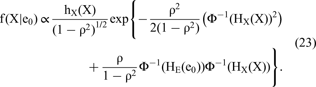
Park and Gupta (2012) employed a JCM approach, positing a GC for the joint CDF of (X, E) as

$$\begin{array}{c}\mathrm{H}(\mathrm{E},\mathrm{X})=\mathrm{C}({\mathrm{H}}_{\mathrm{E}}(\mathrm{E}),{\mathrm{H}}_{\mathrm{X}}(\mathrm{X}))={\mathrm{\Psi }}_{\rho }({\mathrm{\Phi }}^{-1}({\mathrm{H}}_{\mathrm{E}}(\mathrm{E})),{\mathrm{\Phi }}^{-1}({\mathrm{H}}_{\mathrm{X}}(\mathrm{X}))),\end{array}$$

(20)

where H(·,·), H_E(·), and ${\mathrm{H}}_{\mathrm{X}}(\cdot )$ are the CDFs for (E, X), E, and X, respectively; C(·,·) is a bivariate copula function that maps the uniform marginal distributions on [0, 1] to a two-dimensional CDF; and ψ_ρ(·,·) is the CDF of the bivariate standard normal distribution with a Pearson correlation coefficient $\rho$ . The first equation in Equation 20 means that the joint distribution of (E, X) can be written as a copula function C(·,·) of marginal CDFs of E and X, and the second equation assumes a GC function for C(·,·) with the following PDF:

$$\begin{array}{cc}\mathrm{h}(\mathrm{E},\mathrm{X})=\begin{array}{c}{\displaystyle \frac{1}{{(1-{\rho }^2)}^{1/2}}\exp \{-{\displaystyle \frac{{\rho }^2}{2(1-{\rho }^2)}({\mathrm{\Phi }}^{-1}{({\mathrm{H}}_{\mathrm{E}}(\mathrm{E}))}^2+{\mathrm{\Phi }}^{-1}{({\mathrm{H}}_{\mathrm{X}}(\mathrm{X}))}^2)}}\\ +{\displaystyle \frac{\rho }{1-{\rho }^2}{\mathrm{\Phi }}^{-1}({\mathrm{H}}_{\mathrm{E}}(\mathrm{E})){\mathrm{\Phi }}^{-1}({\mathrm{H}}_{\mathrm{X}}(\mathrm{X}))}\}{\mathrm{f}}_{\varphi }(\mathrm{E}){\mathrm{h}}_{\mathrm{X}}(\mathrm{X}),\end{array}& \\ & & & \end{array}$$

(21)

where h_X(X) is the density function of the endogenous regressor X.

Based on the model, Park and Gupta (2012) developed two endogeneity-correction procedures. Both are two-step procedures. In Step 1, one estimates H_X(X) either using empirical CDF or using ${\hat{\mathrm{H}}}_{\mathrm{X}}(\mathrm{X})={\int }_{-\mathrm{\infty }}^{\mathrm{X}}{\hat{\mathrm{h}}}_{\mathrm{X}}(\mathrm{X})$ , where the marginal PDF h_X(·) is estimated using a nonparametric kernel density estimator. In Step 2, the first procedure maximizes the likelihood in Equation 21 in which the estimated CDF ${\hat{\mathrm{H}}}_{\mathrm{X}}(\mathrm{X})$ is plugged in to replace H_X(X). The second procedure adds the latent copula data $\mathrm{X}*={\mathrm{\Phi }}^{-1}({\hat{\mathrm{H}}}_{\mathrm{X}}(\mathrm{X}))$ as a generated regressor into the structural model to control for endogeneity. Because both procedures use the plug-in estimates of distributions for endogenous regressors obtained in Step 1, the usual standard errors in Step 2 underestimate the true sampling variability of model estimates. Park and Gupta (2012) proposed using the bootstrap method to obtain correct standard errors, which requires repeated sampling of the same sample size from the original data and repetition of the preceding estimation procedure on each bootstrap sample.

Advantages of SORE compared with the JCM approach

SORE is more general and flexible than the joint copula approach (Park and Gupta 2012) in the following aspects.

First, SORE nests the joint copula approach as a special case. When (E, X) follows the GC in Equation 21, their joint distribution has the following OR function: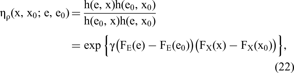

$$\begin{array}{rl}{\eta }_{\rho }(\mathrm{x},{\mathrm{x}}_0;\mathrm{e},{\mathrm{e}}_0)& ={\displaystyle \frac{\mathrm{h}(\mathrm{e},\mathrm{x})\mathrm{h}({\mathrm{e}}_0,{\mathrm{x}}_0)}{\mathrm{h}({\mathrm{e}}_0,\mathrm{x})\mathrm{h}(\mathrm{e},{\mathrm{x}}_0)}}\\ & =\exp \{\gamma \left({\mathrm{F}}_{\mathrm{E}}(\mathrm{e})-{\mathrm{F}}_{\mathrm{E}}({\mathrm{e}}_0)\right)\left({\mathrm{F}}_{\mathrm{X}}(\mathrm{x})-{\mathrm{F}}_{\mathrm{X}}({\mathrm{x}}_0)\right)\},\end{array}$$

(22)

where ${\mathrm{F}}_{\mathrm{E}}(\cdot )={\mathrm{\Phi }}^{-1}({\mathrm{H}}_{\mathrm{E}}(\cdot ))$ and ${\mathrm{F}}_{\mathrm{X}}(\cdot )={\mathrm{\Phi }}^{-1}({\mathrm{H}}_{\mathrm{X}}(\cdot ))$ , and $\gamma =\frac{\rho }{1-{\rho }^2}$ . Thus, the GC model is a special case of the SORE model, where f(X | E) has an OR function specified in Equation 22 and the following specific form of the baseline function:

$$\begin{array}{r}\mathrm{f}(\mathrm{X}|{\mathrm{e}}_0)\propto {\displaystyle \frac{{\mathrm{h}}_{\mathrm{X}}(\mathrm{X})}{{(1-{\rho }^2)}^{1/2}}\exp \{-{\displaystyle \frac{{\rho }^2}{2(1-{\rho }^2)}\left({\mathrm{\Phi }}^{-1}{({\mathrm{H}}_{\mathrm{X}}(\mathrm{X}))}^2\right)}}\\ +{\displaystyle \frac{\rho }{1-{\rho }^2}{\mathrm{\Phi }}^{-1}({\mathrm{H}}_{\mathrm{E}}({\mathrm{e}}_0)){\mathrm{\Phi }}^{-1}({\mathrm{H}}_{\mathrm{X}}(\mathrm{X}))}\}.\end{array}$$

(23)

Similarly, one can show that SORE nests as special cases alternative copulas, such as Placket, Clayton, and Frank copulas. The simulation study in a subsequent section provides further empirical evidence that SORE nests the copula approach as a special case. Thus, SORE is at least as applicable as JCM. Web Appendix C derives SORE for solving slope endogeneity and regressor endogeneity in mixed logit models.

Second, SORE better handles discrete endogenous regressors. Genest and Nešlehová (2007) provide both theoretical results and empirical examples demonstrating that various properties fundamental to copula theory for continuous data are invalidated by discrete data. Specifically, the discreteness in the marginal probability distribution causes plateaus in the inverse of the discrete CDF. Consequently, the nonparametric copula model compatible with data, although it does exist, is not unique and thus encounters model identification issues. This nonidentification issue of the copula for discrete data can cause bias in the estimation of regressor–error dependence, which in turn introduces bias in structural model parameter estimates. This point can be illustrated as follows. Consider using latent copula data ${\mathrm{X}}_{\mathrm{i}}*$ as a generated regressor to handle endogeneity bias. Whereas for a continuous regressor ${\mathrm{X}}_{\mathrm{i}}*={\mathrm{\Phi }}^{-1}({\mathrm{H}}_{\mathrm{X}}({\mathrm{X}}_{\mathrm{i}}))$ , for a discrete regressor we have the following one-to-many mapping from X_i to ${\mathrm{X}}_{\mathrm{i}}*$ (Danaher and Smith 2011; Park and Gupta 2012):

$${\mathrm{\Phi }}^{-1}({\mathrm{H}}_{\mathrm{X}}({\mathrm{X}}_{\mathrm{i}}-1))<{\mathrm{X}}_{\mathrm{i}}*<{\mathrm{\Phi }}^{-1}({\mathrm{H}}_{\mathrm{X}}({\mathrm{X}}_{\mathrm{i}})).$$

(24)

Thus, the copula approach's effectiveness depends on the range of possible values for ${\mathrm{X}}_{\mathrm{i}}*$ and the handling of the mapping. By contrast, SORE includes specifications requiring no inverse mapping of discrete distribution functions and avoids such model nonuniqueness and nonidentifiability issues, as illustrated subsequently using simulated data.

Third, SORE offers certain estimation/inferential advantages. Among the advantages of the one-step SORE estimation mentioned in the introduction to this article, we focus on the direct estimation of standard errors without resorting to bootstrapping. JCM can be estimated in one step by jointly estimating the nonparametric marginal distributions of endogenous regressors and other parameters. However, this is computationally challenging because the likelihood involves a large number of nuisance parameters in the nonparametric marginal distributions, although this can be made easier with density approximation under certain assumptions (Tran and Tsionas 2021). Park and Gupta (2012) estimate the model parameters in two steps, which simplifies estimation, but the inference requires bootstrapped standard errors. The nonparametric marginal-like baseline functions with parameters λ in SORE play the same role as that of the marginal distribution functions of endogenous regressors in JCM. SORE uses a one-step estimation by estimating all model parameters (θ, γ, λ) in one step, ¹⁰ using the profile likelihood to handle nuisance parameters λ. ¹¹ Consequently, uncertainty arising from nonparametric baseline function estimation (i.e., $\hat{\lambda }$ ) is reflected in all model parameters’ likelihood-based standard error estimates.

Considerations in Specifying OR Functions

Since the baseline distribution functions in the SORE model for endogenous regressors are nonparametric, the focus of attention here is on the OR functions that capture regressor–error dependence. Table 2 lists the candidate forms for the logarithm of the OR function ${\eta }_{{\gamma }_{\mathrm{k}}}({\mathrm{x}}_{\mathrm{k}};{\tilde{\mathrm{x}}}_{\mathrm{k}-1},\mathrm{e},\mathrm{w})$ in Equation 11, rewritten as $\ln {\eta }_{{\gamma }_{\mathrm{k}}}({\mathrm{x}}_{\mathrm{k}};\mathrm{e},{\mathrm{z}}_{\mathrm{k}})$ for succinctness with ${\mathrm{z}}_{\mathrm{k}}=({\tilde{\mathrm{x}}}_{\mathrm{k}-1},\mathrm{w})$ containing J variables. Next, we discuss specifications of elements in the OR function and selection among candidate OR functions.

Table 2.

Candidates of OR Functions.

X–E	X–Z	In ${\eta }_{{\gamma }_{\mathbf{k}}}$ (xk; e, zk)
GC	GC	$\left[{\gamma }_{\mathrm{k}}^{\mathrm{E}}({\mathrm{F}}_{\mathrm{E}}(\mathrm{e})-{\mathrm{F}}_{\mathrm{E}}({\mathrm{e}}_0))+\sum _{\mathrm{j}=1}^{\mathrm{J}}{\gamma }_{\mathrm{kj}}^{\mathrm{Z}}({\mathrm{F}}_{{\mathrm{Z}}_{\mathrm{kj}}}({\mathrm{z}}_{\mathrm{kj}})-{\mathrm{F}}_{{\mathrm{Z}}_{\mathrm{kj}}}({\mathrm{z}}_{\mathrm{kj}0}))\right]({\mathrm{F}}_{{\mathrm{X}}_{\mathrm{k}}}({\mathrm{x}}_{\mathrm{k}})-{\mathrm{F}}_{{\mathrm{X}}_{\mathrm{k}}}({\mathrm{x}}_{\mathrm{k}0}))$ Nests existing copula-based IV-free methods as special cases.
GC	LB	${\gamma }_{\mathrm{k}}^{\mathrm{E}}({\mathrm{F}}_{\mathrm{E}}(\mathrm{e})-{\mathrm{F}}_{\mathrm{E}}({\mathrm{e}}_0))({\mathrm{F}}_{{\mathrm{X}}_{\mathrm{k}}}({\mathrm{x}}_{\mathrm{k}})-{\mathrm{F}}_{{\mathrm{X}}_{\mathrm{k}}}({\mathrm{x}}_{\mathrm{k}0}))+\sum _{\mathrm{j}=1}^{\mathrm{J}}{\gamma }_{\mathrm{kj}}^{\mathrm{Z}}({\mathrm{z}}_{\mathrm{kj}}-{\mathrm{z}}_{\mathrm{kj}0})({\mathrm{x}}_{\mathrm{k}}-{\mathrm{x}}_{\mathrm{k}0})$
LB	GC	${\gamma }_{\mathrm{k}}^{\mathrm{E}}(\mathrm{e}-{\mathrm{e}}_0)({\mathrm{x}}_{\mathrm{k}}-{\mathrm{x}}_{\mathrm{k}0})+\sum _{\mathrm{j}=1}^{\mathrm{J}}{\gamma }_{\mathrm{kj}}^{\mathrm{Z}}({\mathrm{F}}_{{\mathrm{Z}}_{\mathrm{kj}}}({\mathrm{z}}_{\mathrm{kj}})-{\mathrm{F}}_{{\mathrm{Z}}_{\mathrm{kj}}}({\mathrm{z}}_{\mathrm{kj}0}))({\mathrm{F}}_{{\mathrm{X}}_{\mathrm{k}}}({\mathrm{x}}_{\mathrm{k}})-{\mathrm{F}}_{{\mathrm{X}}_{\mathrm{k}}}({\mathrm{x}}_{\mathrm{k}0}))$
LB	LB	${\gamma }_{\mathrm{k}}^{\mathrm{E}}(\mathrm{e}-{\mathrm{e}}_0)({\mathrm{x}}_{\mathrm{k}}-{\mathrm{x}}_{\mathrm{k}0})+\sum _{\mathrm{j}=1}^{\mathrm{J}}{\gamma }_{\mathrm{kj}}^{\mathrm{Z}}({\mathrm{z}}_{\mathrm{kj}}-{\mathrm{z}}_{\mathrm{kj}0})({\mathrm{x}}_{\mathrm{k}}-{\mathrm{x}}_{\mathrm{k}0})$

Notes: Causal effect identification assumes the correct OR is in the consideration set and yields an identifiable model, which is weaker than assuming a candidate chosen a priori is correct.

Regressor–error (X–E) dependence

A key element in the OR specification is the X–E dependence. The GC model employed in JCM offers a versatile, robust, and logically consistent way to capture the regressor–error dependence irrespective of marginal distributions. One primary reason for regressor–error dependence is the presence of common omitted variables affecting both regressors and the error. As shown in Web Appendix D.1, when each of the error term and the (unbounded) latent copula data for the endogenous regressors can be expressed as a linear combination of the common omitted variables and a separate white noise term, ¹² then the endogenous regressors and the error term will jointly follow the GC model. In addition to the theoretical plausibility, the GC model is empirically general and robust to capture dependence for most applications (Danaher and Smith 2011) as the model depends on the rank order of raw data only, and is invariant to strictly monotonic transformation of the endogenous regressors and the error. Thus, OR specifications assuming a GC X–E dependence are widely applicable and are good workhorse models for many marketing applications involving continuous endogenous regressors.

Similarly, GLMs are often used to capture nonlinear or nonadditive dependence structures for nonnormal, discrete, or bounded variables that linear additive models cannot handle (McCullagh and Nelder 2019). The LB OR functions for X–E dependence in Table 2 impose no distributional assumptions on endogenous regressors and nest corresponding GLMs as special cases. Because the LB OR functions require no inverse mapping from CDFs of endogenous regressors, they are good starting points for handling discrete endogenous regressors.

Overall, the GC and LB classes of OR functions are both broad, encompassing a number of existing dependence models and providing flexible and logically consistent models for X–E dependence free from constraints in marginal distributions. Model identifiability under these OR functions is established in the “Model Identification” section.

Regressor–Regressor (X–Z) dependence

Relevant regressors in Z should be included in the OR functions to ensure estimation consistency and improve estimation efficiency. Because both X and Z are observed, flexible forms of X–Z dependence can be used to guard against potential misspecifications. One approach is to specify a GC-type X–Z relationship. This is akin to positing a GC model on regressors as is done in Haschka (2022) and Yang, Qian, and Xie (2022). However, SORE is flexible and can model general forms of X–Z dependence using flexible LB OR functions. Even with only first-order terms of regressors, an LB OR function has the flexibility to capture nonlinear effects of Z on the mean of X (Qian and Xie 2022). Furthermore, polynomial or spline terms of regressors in Z can be introduced into the LB OR functions to approximate any smooth nonlinear effects of Z on X, in analogy to nonparametric regression models.

Selection of OR functions

The OR functions in Table 2 can be viewed as different ways to handle regressor endogeneity under different identifying assumptions. Thus, SORE offers a multimethod approach that considers all these OR functions in analysis to check robustness of estimation results. At times, one may need to synthesize results over different OR functions. Theoretical/substantive considerations of the underlying endogeneity problem can guide the process. Prior knowledge of a GC relationship between important omitted variables and endogenous regressors suggests a GC-type regressor–error dependence, whereas knowledge of error heteroskedasticity and/or differences in higher moments suggests that an LB form of regressor–error dependence is more appropriate.

In addition, SORE permits comparison of OR functions using likelihood-based model selection methods. As is always the case, model selection is not error-free (especially when the sample size is not large) and may benefit from incorporating substantive knowledge. The Akaike information criterion (AIC) and Bayesian information criterion (BIC) are the two most commonly used criteria for comparing models (Burnham and Anderson 2004). According to the AIC or BIC, the best-fitting model for each candidate OR function is obtained and compared with each other: the OR function resulting in the smallest AIC or BIC is selected as the best one. Model nonidentification may prevent finding the best-fitting model for an OR function. Causal effect identification assumes that the correct OR is included in the consideration set and yields an identifiable model, which is weaker than assuming any single OR function chosen a priori is correct and identifiable. Under the weaker assumption, any nonidentification of a misspecified OR can only result in a worse AIC or BIC for this misspecified OR and increase the chance that the correct OR is selected. As an unidentified model yields singular Hessian matrix and huge standard error estimates, empirical identification of the model can be checked by inspecting sizes of standard error estimates.

Simulation Studies

In this section, we conduct simulation studies to evaluate the performance of SORE to correct for endogeneity bias, and compare it with the joint modeling approach using GC. Simulation studies have multiple aims. First, because SORE nests JCM as a special case, we expect that its performance is on a par with the copula approach when data follow the copula model. Second, we evaluate SORE and the copula approach under alternative forms of endogeneity. Third, we evaluate SORE's performance for discrete endogenous regressors. Finally, we evaluate SORE's generalizability, flexibility, and robustness under misspecified or nearly unidentified models (Web Appendix D). Throughout the section, correct OR functions are used for estimation, unless noted otherwise.

Handling One Continuous Endogenous Regressor

In this study, we simulated data from two scenarios. In the first scenario, data were simulated from an underlying GC model as follows:

$$(\mathrm{E}*,\mathrm{X}*{)}^{\mathrm{T}}=\mathrm{N}\left({[0,0]}^{\mathrm{T}},\left[\begin{array}{cc}1& \rho \\ \rho & 1\end{array}\right]\right),$$

(25)

$$\mathrm{E}={\mathrm{H}}_{\mathrm{E}}^{-1}\left(\mathrm{\Phi }(\mathrm{E}*)\right)={\mathrm{\Phi }}_{(0,{\sigma }^2)}^{-1}\left(\mathrm{\Phi }(\mathrm{E}*)\right),\mathrm{X}={\mathrm{H}}_{\mathrm{X}}^{-1}\left(\mathrm{\Phi }(\mathrm{X}*)\right),$$

(26)

$$\mathrm{Y}=\mu +\alpha \mathrm{X}+\mathrm{E}.$$

(27)

In the simulation, we set H_X(·) to be the CDF of the truncated standard normal with a lower bound of 0, α = −1, μ = 0, σ = 1, and ρ = .5 with sample size varying between 200, 1,000, and 5,000. The GC model is a special case of the SORE model for (X, E) where f(X | E) follows a SORE model with the OR function and the baseline function f(X | e₀) given in Equations 22 and 23, respectively. In this case, we expect that both JCM and SORE with the OR function in Equation 22 can correct for endogeneity.

Results from 1,000 simulated samples are summarized in Table 3 in the “Under JCM Models” column. As expected, the OLS estimation yields large bias for the estimates of the structural model parameters (α, μ, σ). The ratio of the size of bias (i.e., the absolute difference between the true parameter values and the means of estimates) to the standard error, reported in the “t_bias” column, shows a large bias (t_bias >> 2) for all sample sizes. By contrast, both the copula and SORE eliminate the endogeneity bias. SORE has somewhat less variability of the estimates for (θ, γ), indicating greater estimation efficiency relative to the two-step estimation used in the copula approach. Table 3 also shows that the standard error estimates (in parentheses) computed from the Hessian matrix of the SORE model are close to the true standard errors.

Table 3.

Comparison of Estimation Methods with a Continuous Endogenous X.

Method	N	Parameter	TrueValues	Under JCM Models			Under SORE Models
				Mean	SE	tbias	Mean	SE	tbias
OLS	200	$\alpha$	−1	−.205	.106	7.5	.243	.077	16.0
		$\mu$	0	−.643	.104	6.2	−.728	.075	9.7
		$\sigma$	1	.873	.044	2.9	.665	.038	8.8
		$\gamma$	.667 (1) a	—	—	—	—	—	—
	1,000	$\alpha$	−1	−.199	.048	16.7	.241	.034	36.5
		$\mu$	0	−.636	.049	13.0	−.724	.029	25.0
		$\sigma$	1	.876	.020	6.2	.667	.016	20.8
		$\gamma$	.667 (1) a	—	—	—	—	—	—
	5,000	$\alpha$	−1	−.202	.021	38.1	.239	.015	82.6
		$\mu$	0	−.638	.020	31.9	−.721	.014	51.5
		$\sigma$	1	.876	.009	13.8	.666	.007	47.7
		$\gamma$	.667 (1) a	—	—	—	—	—	—
JCM	200	$\alpha$	−1	−.972	.408	.1	−.208	.198	4.0
		$\mu$	0	−.010	.351	.0	−.470	.121	3.9
		$\sigma$	1	1.013	.125	.1	.729	.064	4.2
		$\gamma$	.667 (N.A.) a	.698	.463	.1	.462	.226	N.A.
	1,000	$\alpha$	−1	−.995	.176	.0	−.212	.085	9.3
		$\mu$	0	.007	.150	.0	−.465	.061	7.6
		$\sigma$	1	1.003	.055	.1	.721	.025	11.2
		$\gamma$	.667 (N.A.) a	.678	.183	.1	.443	.094	N.A.
	5,000	$\alpha$	−1	−1.002	.079	.0	−.210	.037	21.4
		$\mu$	0	.002	.070	.0	−.458	.025	18.3
		$\sigma$	1	1.001	.025	.0	.719	.012	23.4
		$\gamma$	.667 (N.A.) a	.667	.081	.0	.442	.041	N.A.
SORE	200	$\alpha$	−1	−.981	.397 (.391)	.1	−.996	.177 (.170)	.0
		$\mu$	0	−.016	.330 (.324)	.0	−.011	.119 (.119)	.1
		$\sigma$	1	1.002	.114 (.111)	.1	.994	.090 (.090)	.1
		$\gamma$	.667 (1) a	.661	.339 (.330)	.0	1.003	.189 (.187)	.0
	1,000	$\alpha$	−1	−1.002	.173 (.169)	.0	−.997	.076 (.075)	.0
		$\mu$	0	.002	.143 (.139)	.0	−.010	.050 (.052)	.2
		$\sigma$	1	1.002	.054 (.053)	.0	.998	.041 (.041)	.0
		$\gamma$	.667 (1) a	.668	.143 (.140)	.0	.987	.082 (.081)	.2
	5,000	$\alpha$	−1	−.996	.076 (.075)	.1	−.998	.034 (.034)	.1
		$\mu$	0	−.005	.062 (.062)	.1	−.002	.023 (.024)	.1
		$\sigma$	1	.998	.024 (.024)	.1	.999	.018 (.018)	.1
		$\gamma$	.667 (1) a	.661	.063 (.062)	.1	.991	.036 (.036)	.3

^a

The association between the endogenous regressor X and structural error is parameterized as γ, which has a true value of $\frac{\rho }{1-{\rho }^2}\approx .667$ when data were generated from the GC model with ρ = .5, and has a true value of 1 when data were generated from the SORE model. The estimate of γ using the copula method is $\frac{\hat{\rho }}{1-{\hat{\rho }}^2}$ , where $\hat{\rho }$ is the copula estimate of ρ.

Notes: Unless noted otherwise, the tables for simulation studies report the mean, standard deviation of estimates (SE), and relative bias (t_bias) of the estimates over repeated samples. The average standard error estimates over the repeated samples using inverse Hessian matrix of the SORE model are reported in parentheses in the “SE” column. N.A. = not applicable.

In the second scenario, data were simulated in three steps: (1) generate E from N(0, σ²); (2) given E, generate X from a truncated normal distribution $(\mathrm{X}=\mathrm{x}|\mathrm{E}=\mathrm{e})\sim \mathrm{TN}({\mu }_{\mathrm{x}|\mathrm{e}},$ ${\sigma }_{\mathrm{x}}^2,\mathrm{lb}=0)$ , where μ_x|e = λ₀ + γe, and X > lb; and (3) given E = e and X = x, generate y = μ + αx + e. We set σ = 1, σ_x = .5, λ₀ = 0, γ = 1, α = −1, and μ = 0. The truncated normal regression in Step 2 can be reexpressed as a SORE with the OR function

$$\ln (\eta (\mathrm{x};\mathrm{e}))={\gamma }^{\mathrm{E}}(\mathrm{x}-{\mathrm{x}}_0)(\mathrm{e}-{\mathrm{e}}_0),$$

(28)

where ${\gamma }^{\mathrm{E}}=\gamma /{\sigma }_{\mathrm{x}}^2$ , and the baseline distribution X | (E = e₀) follows a parametric truncated normal distribution $\mathrm{TN}({\mu }_{\mathrm{x}|{\mathrm{e}}_0},{\sigma }_{\mathrm{x}}^2,\mathrm{lb}=0)$ , where ${\mu }_{\mathrm{x}|{\mathrm{e}}_0}={\lambda }_0+\gamma {\mathrm{e}}_0$ .

Results across 1,000 samples show that OLS yields significant bias for model parameter estimates (see the “Under SORE Models” column in Table 3). The copula reduces the bias of the OLS estimates to some extent, but significant bias remains.

Figure 1 plots transformed data X* = Φ⁻¹(H_X(X)) and E* = E for a random sample of 1,000 observations on X and E simulated using the three-step procedure outlined previously. A nonparametric locally estimated scatterplot smoothing (LOESS) regression line is also plotted, which shows a marked departure from the straight regression line expected if (X*, E*) follows a bivariate normal distribution. In this case, GC misspecifies the true dependence structure between X and E. The misspecification using GC results in the appreciable bias in model parameter estimates observed in Table 3.

Figure 1.

Plot of Latent Copula Data.

By contrast, SORE with the OR function in Equation 28 properly models regressor–error dependence and consequently eliminates the endogeneity bias (Table 3). This demonstrates SORE's flexibility in handling alternative forms of endogeneity. Figure 2 plots the residuals from a LOESS regression of E on X for a random sample of 1,000 observations, demonstrating heteroskedasticity in ${\sigma }_{\mathrm{e}|\mathrm{x}}^2$ for model identification (Proposition 1).

Figure 2.

Heteroskedasticity.

Comparison of the OR Functions

As noted in the “Considerations in Specifying OR Functions” section, statistical model selection measures can be a useful tool to aid the OR function specifications. To evaluate the feasibility and effectiveness of using model selection measures to aid the OR function specifications, we conducted the following study.

We simulated data from models in Equations 25–27 for a sample size of 1,000. For each data set, we fit two SORE models: one with the correct OR function in Equation 8, denoted as “SORE^C,” and the other one, denoted as “SORE^M,” with the following misspecified OR function: ln(η(x; e)) = γ(x − x₀)(e − e₀). We then compute AICs and BICs of SORE^C and SORE^M, and the model with the smaller AIC or BIC is selected. We repeat the model estimation and comparison for 1,000 generated samples. Table 4 shows that over 1,000 simulated data sets of sample size N = 1,000, the AIC of SORE^C on average is lower than that of SORE^M by 8,706.1 − 8,689.8 = 16.3 (and for the BIC, by 8,871.9 − 8,855.6 = 16.3). In 98.4% of 1,000 simulated data sets, SORE^C has a lower AIC or BIC than SORE^M and is selected as the correct one. Table W14 in Web Appendix D.10 shows that SORE^M with an incorrect OR cannot remove all the endogeneity bias in OLS estimates, resulting in biased parameter estimates and inconsistent likelihood-based standard error estimates, whereas SORE^C using the correct OR yields consistent parameter estimates and standard error estimates. Overall, the finding that the AIC or BIC almost surely selects the correct OR in large samples demonstrates the feasibility of model selection measures to aid correct OR specification.

Table 4.

Comparison of OR Functions.

N	Measures	SOREM	SOREC
200	Avg. AIC (BIC)	1,756.4 (1,848.9)	1,753.9 (1,846.3)
	% selected	20.3% (20.3%)	79.7% (79.7%)
500	Avg. AIC (BIC)	4,364.8 (4,396.9)	4,357.0 (4,489.1)
	% selected	4.7% (4.7%)	95.3% (95.3%)
1,000	Avg. AIC (BIC)	8,706.1 (8,871.9)	8,689.8 (8,855.6)
	% selected	1.6% (1.6%)	98.4% (98.4%)

The effectiveness of comparing different OR functions using the AIC or BIC depends on information contained in the data to distinguish different endogeneity models. Table 4 reports results for sample sizes N = 200 and N = 500. Although SORE^C continues to have a lower average AIC (BIC) than SORE^M, the average difference in AIC (or BIC) between SORE^M and SORE^C becomes smaller for a smaller sample size. For a small sample size (N = 200), AIC or BIC selects the correct OR in 79.7% of 1,000 simulated data sets. This is expected because a smaller sample contains less information to distinguish different OR functions.

Correlated Exogenous and Endogenous Regressors and Comparison to IVs

We simulated data from the following joint model:

$$(\mathrm{E}*,\mathrm{X}*,\mathrm{W}*,\mathrm{Z}{)}^{\mathrm{T}}=\mathrm{N}\left({[0,0,0,0]}^{\mathrm{T}},\left[\begin{array}{cccc}1& .5& 0& 0\\ .5& 1& .5& .5\\ 0& .5& 1& .5\\ 0& .5& .5& 1\\ & & & \end{array}\right]\right),$$

(29)

$$\begin{array}{r}\mathrm{E}={\mathrm{H}}_{\mathrm{E}}^{-1}\left(\mathrm{\Phi }(\mathrm{E}*)\right)={\mathrm{\Phi }}^{-1}\left(\mathrm{\Phi }(\mathrm{E}*)\right),\\ \mathrm{X}={\mathrm{H}}_{\mathrm{X}}^{-1}\left(\mathrm{\Phi }(\mathrm{X}*)\right),\mathrm{W}={\mathrm{H}}_{\mathrm{W}}^{-1}\left(\mathrm{\Phi }(\mathrm{W}*)\right),\end{array}$$

(30)

$$\mathrm{Y}=\mu +\alpha \mathrm{X}+\beta \mathrm{W}+\mathrm{E}.$$

(31)

We set H_X(·) as the CDF of the truncated standard normal with a lower bound of 0 and H_W(·) as the CDF of the exponential distribution with the rate of 1 and sample size 1,000. For each data set, we apply OLS, copula, two-stage least squares (TSLS), and SORE. TSLS uses Z as an IV: Z is uncorrelated with E and does not directly affect Y (i.e., exclusion restriction) and is correlated with X (i.e., relevant). The JCM models (E, X) jointly using the GC in Equation 21. By contrast, SORE models the conditional distribution (E, X) | W and accounts for the correlation between W and X. SORE uses the following OR:

$$\begin{array}{rl}\ln {\eta }_{\gamma }(\mathrm{x};\mathrm{w},\mathrm{e})=& {[\gamma }^{\mathrm{W}}({\mathrm{F}}_{\mathrm{W}}(\mathrm{w})-{\mathrm{F}}_{\mathrm{W}}({\mathrm{w}}_0))\\ & +{\gamma }^{\mathrm{E}}({\mathrm{F}}_{\mathrm{E}}(\mathrm{e})-{\mathrm{F}}_{\mathrm{E}}({\mathrm{e}}_0))]\left({\mathrm{F}}_{\mathrm{X}}(\mathrm{x})-{\mathrm{F}}_{\mathrm{X}}({\mathrm{x}}_0)\right),\end{array}$$

(32)

where F_X(·) and F_W(·) denote normal score transformations of X and W, respectively, and ${\mathrm{F}}_{\mathrm{E}}(\cdot )={\mathrm{\Phi }}_{(0,{\hat{\sigma }}^2)}^{-1}(\mathrm{\Phi }(\cdot ))$ . Results across 1,000 simulated samples show considerable bias for OLS (Table 5). Substantial bias also exists in the JCM approach that ignores the correlation between X and W. By contrast, SORE accounts for this correlation and yields consistent parameter estimates with smaller SEs, demonstrating the ability of SORE to improve estimation by making use of relevant exogenous regressors. TSLS also corrects for endogeneity bias, yielding consistent estimates with somewhat larger SEs than those of SORE. This shows that SORE can perform as well as TSLS. Unlike TSLS, however, SORE is applicable when no IV is available.

Table 5.

Estimation with Correlated X and W.

	TrueValues	OLS			JCM			TSLS			SORE
		Mean	SE	tbias	Mean	SE	tbias	Mean	SE	tbias	Mean	SE	tbias
α	1	2.02	.05	20.3	1.17	.18	1.0	1.00	.18	.0	1.00	.15 (.14)	.1
μ	1	.48	.05	11.7	1.15	.15	1.0	1.00	.10	.0	1.00	.09 (.09)	.0
β	−1	−1.29	.03	9.2	−1.29	.03	9.1	−1.00	.06	.0	−1.00	.05 (.05)	.1
σ	1	.84	.02	8.5	.99	.06	.3	1.00	.06	.0	1.00	.05 (.05)	.0
γW	1	—	—	—	—	—	—	—	—	—	1.00	.10 (.10)	.0
γE	1	—	—	—	.76	.20	1.2	—	—	—	1.00	.15 (.14)	.0

Handling One Binary Endogenous Regressor

To examine SORE's ability to handle binary endogenous regressors, we performed the following simulation study. In the first scenario, data were simulated in three steps: (1) generate E from N(0, σ²); (2) given E, generate X from a binary logistic regression model: logit(P(X = 1 | E = e)) = λ₀ + γe; and (3) given E = e and X = x, generate Y = μ + αx + e. We set σ = 2, λ₀ = −2, γ = 2, α = 1, and μ = 0. The binary logit model in Step 2 is a SORE model with the OR function ln(η(x; e)) = γ(x − x₀)(e − e₀) and the baseline distribution f(X | E = e₀) following a Bernoulli distribution with logit(P(X = 1 | E = e)) = λ₀ + γe₀.

Results across 1,000 simulated samples with sample size 200 and 1,000, reported in Table 6 in the “Under SORE Model” column, show that (1) the OLS estimates exhibit large bias, and (2) using the OR function ln(η(x; e)) = γ(x − x₀)(e − e₀), SORE detects endogeneity and corrects for endogeneity bias. As a large-sample procedure, SORE may encounter weak identification with nearly flat likelihood in small samples even when the OR function is correctly specified. For the smaller sample size (N = 200) with a binary endogenous regressor, 2 out of 1,000 generated data sets in our simulation yield almost unidentified models with huge Hessian-based standard error estimates (155.6 and 170.3) for $\hat{\alpha }$ . As SORE should not be used in data with such huge standard error estimates, we exclude these two problematic data sets and evaluate SORE's performance in the remaining 998 data sets. We encountered no such problematic data sets for sample size N = 1,000, and all generated data sets are used in evaluation. Although results are not reported here, JCM cannot detect endogeneity and yields estimates with similar bias as OLS does. Park and Gupta (2012) noted JCM's inability to handle binary endogenous regressors as a limitation. The simulation study demonstrates that SORE overcomes JCM's limitation in handling binary endogenous regressors and can correct for endogeneity bias for binary endogenous regressors. The theoretical reason is that unlike JCM, SORE has specifications requiring no inverse mapping from discrete CDFs.

Table 6.

Estimation for Binary Endogenous X.

Param.	Under SORE Model						Under Copula Model
	OLS			SOREC			OLS			SOREM
	Mean	SE	tb	Mean	SE	tb	Mean	SE	tb	Mean	SE a	tb
N = 200
α = 1	3.99	.21	14.2	1.02	.37 (.37)	.1	2.59	.26	6.1	1.20	1.36 (3.55)	.1
μ = 0	−.97	.13	7.4	−.01	.19 (.19)	.1	−.80	.18	4.4	−.10	.69 (1.83)	.1
σ = 2	1.42	.08	7.3	2.00	.16 (.16)	.1	1.82	.09	2.0	2.04	.27 (.28)	.1
γ = 2 (.67)	—	—	—	2.15	.54 (.52)	.2	—	—	—	.43	.44 (1.16)	.5
N = 1,000
α = 1	4.00	.09	33.3	1.01	.16 (.16)	.1	2.59	.11	14.5	1.30	1.03 (1.44)	.3
μ = 0	−.98	.08	12.3	−.01	.08 (.08)	.1	−.79	.08	9.9	−.15	.52 (.72)	.3
σ = 2	1.43	.03	18.9	2.00	.07 (.07)	.1	1.83	.04	4.4	2.00	.17 (.17)	.0
γ = 2 (.67)	—	—	—	2.02	.20 (.20)	.1	—	—	—	.39	.31 (.44)	.9

^a

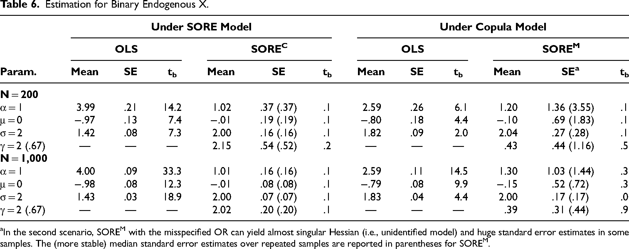
In the second scenario, SORE^M with the misspecified OR can yield almost singular Hessian (i.e., unidentified model) and huge standard error estimates in some samples. The (more stable) median standard error estimates over repeated samples are reported in parentheses for SORE^M.

In the second scenario, we simulated data from the copula model specified in Equations 25 to 27 except with X being binary and generated as X = 1 (0) if X* > 0 (< 0). This means H_X(X = 0) = .5 and H_X(X = 1) = 1. In the simulation, we set μ = 0, α = 1, σ = 2, and ρ = .5. Results across 1,000 simulated samples are reported in Table 6 in the “Under Copula Model” column and show that (1) the OLS estimates exhibit large bias, and (2) using the OR function ln(η(x; e)) = γ(x − x₀)(e − e₀), SORE reduces the bias in OLS estimates but significant bias remains. Similar to the first scenario shown previously, JCM cannot detect endogeneity and yields estimates with similar bias as OLS does. As Web Appendix E shows, the OR used previously in SORE is misspecified in the second scenario. With the misspecified OR function, estimation bias occurs and the standard error estimate for α in SORE is huge (approximately ten times of that of OLS estimates), suggesting model nonidentification issues. Thus, the simulation study illustrates the importance of correctly specifying OR functions and checking standard error estimates to detect potential OR misspecifications.

Additional Simulation Results

We conduct additional simulation studies to evaluate the generalizability, flexibility, and robustness of the proposed SORE methods. In Web Appendix D.1, we describe and demonstrate SORE's capability to handle omitted variables, reverse causality, and simultaneity. We further show that SORE can successfully correct for endogeneity bias for the cases of count endogenous regressors (Web Appendix D.2), endogenous regressors with mixture normal distributions (Web Appendix D.3), multiple endogenous regressors (Web Appendix D.4), and slope endogeneity (Web Appendix D.5). As shown in Becker, Proksch, and Ringle (2021), JCM can be subject to considerable estimation bias in finite samples when the structural model includes an intercept. Using exactly the same setting as Becker, Proksch, and Ringle, the simulation study in Web Appendix D.6 shows that SORE is free from the bias issue encountered by JCM, albeit having substantially larger standard errors when the sample size is small. We also consider the case of linear endogeneity in which a nonnormal endogenous regressor contains a normally distributed additive component causing regressor–error dependence. Haschka (2022) shows that, interestingly, JCM cannot handle linear endogeneity, resulting in bias opposite to that of OLS estimates with huge standard errors relative to those from the OLS estimation. Web Appendix D.7 shows that, like JCM, SORE is subject to the same model nonidentification issue (hugely inflated standard errors). Although such linear endogeneity is unlikely to hold in many empirical applications as noted in Web Appendix D.7, it is important to check model identification and inspect standard error estimates for signs of contraindications of SORE.

We also conduct simulation studies to evaluate the robustness of SORE to modeling assumptions. Web Appendix D.8 assesses the robustness of SORE to the assumption of normal error distributions. We find that SORE yields biased estimates and standard error estimates when the error distribution is skewed or has fat tails. SORE performs well for symmetric nonnormal error distributions without fat tails, yielding unbiased estimates with consistent standard error estimates. Web Appendix D.9 assesses the performance of unidentified SORE models. The adverse effects of unidentified SORE models include biased estimates centered at the OLS estimates and huge standard errors of the coefficients of endogenous regressors relative to those of OLS estimates. The latter adverse effect (huge standard error) can be used as a diagnostic tool to indicate the presence of empirically unidentified models. We also investigate the robustness of OR selection to error distribution misspecifications and find that OR selection using AIC or BIC is robust to symmetric nonnormal distributions and asymmetric nonnormal error distributions (Web Appendix D.11). Web Appendix D.12 shows that OR comparison can select the correct one with multiple and correlated endogenous regressors and that the misspecification of OR causes bias primarily on the coefficient of the endogenous regressor whose OR is misspecified.

Empirical Application

In this section, we apply SORE to the store sales data set used by Park and Gupta (2012) to demonstrate using JCM to handle price endogeneity when estimating the demand for paper towels. Our illustration aims to demonstrate the capability of SORE to (1) model more general forms of regressor endogeneity than that modeled by JCM, and (2) handle discrete endogenous regressors with a small number of levels that JCM is not designed for.

Handling Continuous Endogenous Regressors

The received data set ¹³ includes weekly store-level sales, retail price (price per roll of paper towels), feature advertising, and in-store display of paper towels at the category level for the two largest independent stores in Eau Claire, Wisconsin, from 2001 to 2005. All the preceding category-level variables (sales, retail price, feature advertising, and in-store display) are computed as market-share weighted averages of the respective Universal Product Code–level variables and take on continuous values. As in Park and Gupta (2012), we estimate the following demand model:

$$\begin{array}{c}\ln (\mathrm{Sale}{\mathrm{s}}_{\mathrm{i}})=\mu +\alpha \cdot \ln (\mathrm{RetailPric}{\mathrm{e}}_{\mathrm{i}})+{\mathrm{W}}_{\mathrm{i}}^{\mathrm{T}}\beta +{\mathrm{E}}_{\mathrm{i}},\end{array}$$

(33)

where i indexes the week, and the vector W_i includes Promotion (feature advertising), Display, and three dummy variables representing quarters Q2, Q3, and Q4. Following Park and Gupta, we treat Promotion and Display as exogenous variables; prior research has shown that advertising endogeneity is highly unlikely for weekly data (Becker, Wiegand, and Reinartz 2019; Sriram, Balachander, and Kalwani 2007). In the data set, the log retail price is time detrended to eliminate an increasing trend of retail price over the five-year study period. Henceforth, for succinctness, we use Price to denote ln(RetailPrice).

The endogeneity of retail price can occur because of unobserved product attributes or demand shocks that affect consumer demand and retailer pricing decisions. These unobservables are absorbed into E_i, causing the price–error dependence and the endogeneity of retail price. Thus, the OLS estimates of the preceding demand model are subject to potential endogeneity bias. Subsequently, we apply SORE to correct for potential price endogeneity, using the TSLS estimator as the benchmark to assess SORE's performance. As in Park and Gupta (2012), TSLS estimation uses the log retail price at the other store as an instrument for the log retail price at the focal store. Prices of the paper towels at the two stores are highly correlated (Pearson correlation coefficient = .83) because the two stores typically have similar wholesale product prices. Meanwhile, unobserved product attributes, including retailer decisions about shelf location and facings, are unlikely to be related to wholesale prices. Under this assumption, the log retail price at the other store can serve as a valid IV for the endogenous log retail price at the focal store in the estimation.

SORE requires no IVs. Like JCM, however, SORE requires modeling regressor–error dependence and sufficient nonnormality of the endogenous regressor (Corollaries 2 and 3 in Web Appendix B). The distributions of the log retail price at the two stores are both left-skewed and reject normality at the .01 level for both Shapiro–Wilk and Kolmogorov–Smirnov tests, suggesting that the log retail prices at the two stores are not normally distributed. Compared with JCM, SORE achieves identification under the weaker assumption that price endogeneity is of a form in the set of OR functions considered in Table 7, which include JCM as special cases. These OR functions relax the assumption of GC regressor–error dependence and the assumption of independence or GC relationship between exogenous and endogenous regressors imposed in JCM and its recent extensions. Meanwhile, the assumption that the regressor–error dependence follows either a GC or an LB structure is untestable. As noted in the “Considerations in Specifying OR Functions” section, these two classes of structures cover broad types of regressor–error dependence unconstrained by marginal distributions of endogenous regressors; they cover the widely applicable GC dependence and broaden it to even greater scopes of regressor endogeneity. Specifically, that section shows that GC dependence is a plausible model for explaining regressor endogeneity due to omitted variables. Furthermore, as shown in Web Appendix D.1, regressor–error dependence follows the GC OR function when the regressor (price here) and these omitted variables (or a linear combination of these variables) jointly follow a GC model. This assumption is empirically plausible given that the GC model is flexible and applicable in many marketing applications to capture relationships among variables (Danaher and Smith 2011; Eckert and Hohberger 2023; Park and Gupta 2012). Meanwhile, because GLMs are frequently used to model dependence in practical data analysis, it is also plausible to assume that the error term relates to the price via an LB OR function, which captures price–error dependence via distribution-free GLMs for dependence and, like the GC model, captures the dependence irrespective of marginal distributions.

Table 7.

Model Selection.

SORE Model	Dependence Structure in OR		Store 1		Store 2
	Price–E	Price–W	MLL	AIC	MLL	AIC
M1	LB	LB	−683.85	1,395.70a	−668.41	1,364.82a
M2	GC	LB	−687.63	1,403.26b	−669.44	1,366.88b
M3	GC	GC	−701.47	1,430.94	−682.50	1,393.00
M4	LB	GC	−701.80	1,431.60	−682.51	1,393.02
M5	GC	Independent	−764.68	1,547.36	−721.05	1,460.10
M6	LB	Independent	−765.80	1,549.60	−721.11	1,460.22

^aModel with smallest AIC.

^bModel with second smallest AIC.

Notes: MLL = maximized log-likelihood. AIC = 2d − 2MLL, where d is the dimension of (θ, γ). BIC yields the same model selection results as AIC and is thus not presented. M5 and M3 yield SORE counterparts of JCM and its extensions assuming GC regressor–regressor dependence, respectively.

To select proper OR functions, we adopt a standard model selection approach that treats all OR functions in Table 7 as equally possible a priori, and relies on the AIC or BIC to select OR functions. ¹⁴ Propositions in the “Model Identification” section inform the sources of identifications for the selected OR functions. It is important to check whether empirical identification is achieved for particular OR functions given the data at hand. We will inspect standard errors from SORE with the selected OR functions to verify empirical identification and check for signs of weakly identified or unidentified models or misspecified regressor–error dependence.

The OR functions in Table 7 permit both GC and non-GC (LB) dependence for both regressor–error (Price–E) and regressor–regressor (Price–W) relationships. For example, M2 in Table 7 specifies GC Price–E dependence and LB Price–W dependence with

$$\begin{array}{rl}\ln {\eta }_{\gamma }(\mathrm{Pric}{\mathrm{e}}_{\mathrm{i}};{\mathrm{E}}_{\mathrm{i}},{\mathrm{W}}_{\mathrm{i}})=& {\gamma }^{\mathrm{E}}({\mathrm{F}}_{\mathrm{P}}(\mathrm{Pric}{\mathrm{e}}_{\mathrm{i}})-{\mathrm{F}}_{\mathrm{P}}(\mathrm{Pric}{\mathrm{e}}_0))({\mathrm{F}}_{\mathrm{E}}({\mathrm{E}}_{\mathrm{i}})-{\mathrm{F}}_{\mathrm{E}}({\mathrm{E}}_0))\\ & +\sum _{\mathrm{q}=1}^{\mathrm{Q}}{\gamma }_{\mathrm{q}}^{\mathrm{W}}(\mathrm{Pric}{\mathrm{e}}_{\mathrm{i}}-\mathrm{Pric}{\mathrm{e}}_0)({\mathrm{W}}_{\mathrm{iq}}-{\mathrm{W}}_{\mathrm{q}0}),\end{array}$$

(34)

where Price stands for detrended log retail price; γ^E and ${\gamma }_{\mathrm{q}}^{\mathrm{W}}$ capture Price–error dependence and Price–W_q dependence, respectively, where W_iq is the qth element in W_i. Notably, γ^E measures the strength of price endogeneity, conditioning on the exogenous regressors in W. When ${\gamma }_{\mathrm{q}}^{\mathrm{W}}=0$ for all q = 1 to Q, ln η_γ(Price_i; E_i, W_i) = γ^E(F_p(Price_i) − F_p(Price₀))(F_E(E_i) − F_E(E₀)), yielding M5 in Table 7, which has the same OR function as that of JCM. Thus, JCM is a special case of SORE: while SORE permits potential correlations of Price with exogenous regressors W via ${\gamma }_{\mathrm{q}}^{\mathrm{W}}$ , JCM implicitly assumes all ${\gamma }_{\mathrm{q}}^{\mathrm{W}}$ s are fixed at zero (i.e., independence of exogenous and endogenous regressors), which, if incorrect, may cause bias, as shown previously in our simulation study. We also add higher-order terms of Promotion and Display (up to the fourth power) and their cubic spline terms into W, and find none of these higher-order terms and spline terms to be statistically significant. Thus, we include only the first-order term of exogenous regressors in the LB form of Price–W dependence. We also consider GC Price–W dependence by replacing Price and W_q with their normal score transformations in Equation 34, yielding M3 in Table 7, which has the same OR function as that of Haschka (2022), assuming a GC for the error term and all regressors. We standardize all regressors and the error term, which makes γ^E more comparable but otherwise has no effect on the SORE estimation. A nonparametric baseline function for the endogenous regressor Price is used in SORE.

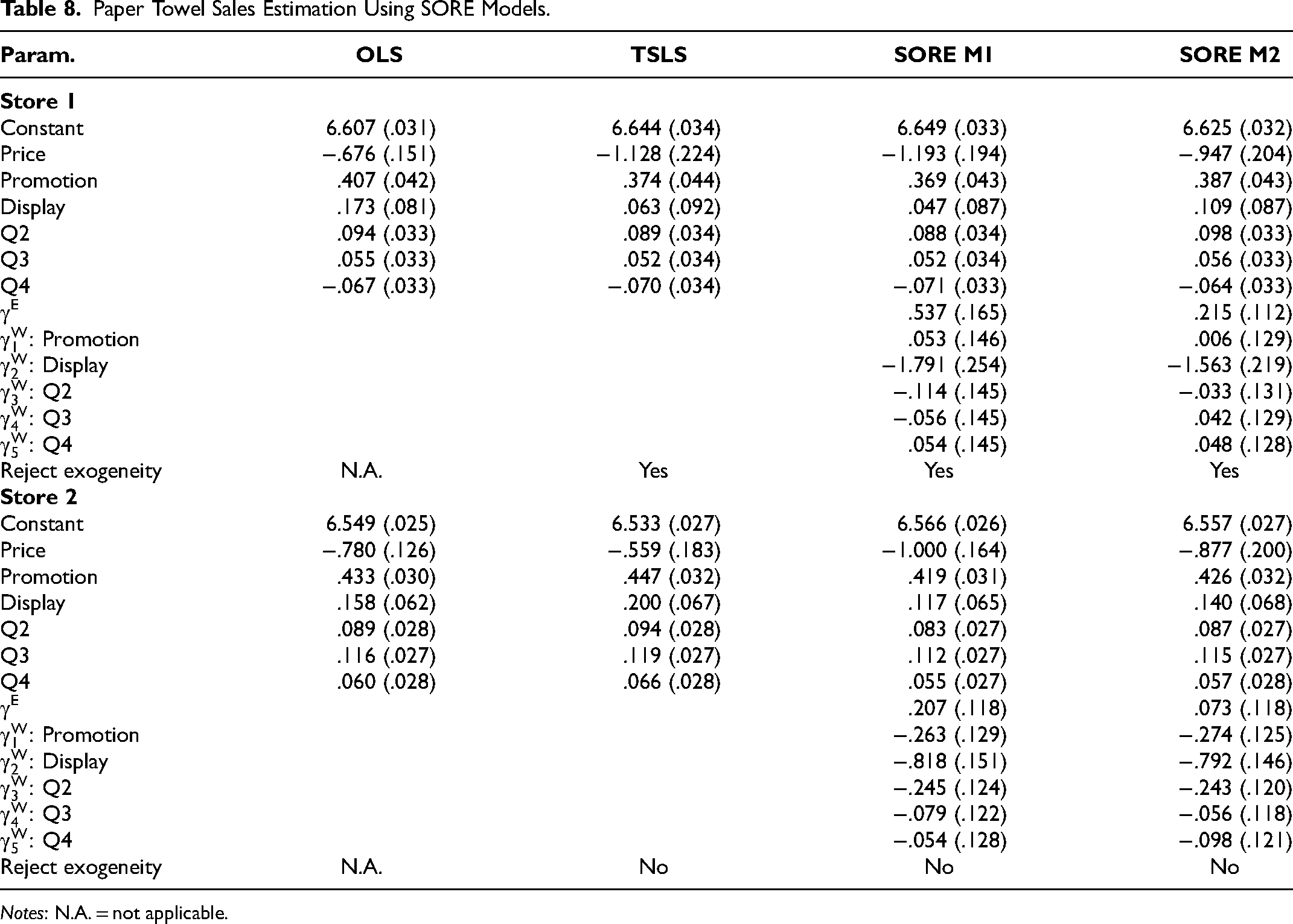
Table 7 reports AICs for all SORE models. For the ith SORE model in Table 7, we define Δ_i = AIC_i − AIC_min, where AIC_i and AIC_min denote AIC for the ith model and the best model in the consideration set, respectively. A rule of thumb is that models with Δ_i < 2 have strong data support; models with 4 ≤ Δ_i ≤ 7 have considerably less support; and models with Δ_i > 10 have no support (Burnham and Anderson 2004). Table 7 shows that M1 has the smallest AIC and is the best model. According to the rule, the SORE model M2, the second best model, yields a comparable AIC as the best model in Store 2 (Δ_i ≈ 2), and less so in Store 1 but cannot be ruled out (Δ_i ≈ 7). Interestingly, SORE M1 has smaller AICs than M2, suggesting that LB explains regressor–error dependence better than GC. All other SORE models have no support (Δ_i > 10). Table 8 reports the estimation results of M1 and M2 together with OLS and TSLS. Our implementation of TSLS using Stata yields price estimates that are consistent with those reported in the original article on the direction of potential bias in the OLS estimates but with somewhat different sizes. For Store 1, the OLS, TSLS, SORE M1, and SORE M2 estimates (with standard errors in parentheses) for the price coefficient are −.676 (.151), −1.128 (.224), −1.193 (.194), and −.947 (.204), respectively. JCM yields a similar estimate to that of SORE M2 and so is not reported. The price coefficient from OLS is substantially greater than that from TSLS, suggesting the presence of price endogeneity. The Hausman test for endogeneity from TSLS also confirms price endogeneity (p = .004). The OLS price coefficient estimate is biased likely because the unmeasured product characteristics captured in E can cause a positive correlation between E and Price, leading to upward bias (meaning less consumer price sensitivity) in the OLS estimate of the price coefficient. Price coefficient estimates from both SORE M1 and M2 show greater price sensitivity than the OLS estimate, suggesting that both models correct price endogeneity. SORE M1's price estimate (−1.193) is closer to the TSLS price coefficient estimate (−1.128), consistent with the fact that M1 outperforms M2 in AIC. In fact, 95% CIs for the price coefficient estimate from both TSLS and SORE M1 exclude the OLS estimate, whereas that from SORE M2 does not. The standard errors of SORE models are comparable to those of TSLS and only slightly larger than those of OLS, showing no signs of weak identification.

Table 8.

Paper Towel Sales Estimation Using SORE Models.

Param.	OLS	TSLS	SORE M1	SORE M2
Store 1
Constant	6.607 (.031)	6.644 (.034)	6.649 (.033)	6.625 (.032)
Price	−.676 (.151)	−1.128 (.224)	−1.193 (.194)	−.947 (.204)
Promotion	.407 (.042)	.374 (.044)	.369 (.043)	.387 (.043)
Display	.173 (.081)	.063 (.092)	.047 (.087)	.109 (.087)
Q2	.094 (.033)	.089 (.034)	.088 (.034)	.098 (.033)
Q3	.055 (.033)	.052 (.034)	.052 (.034)	.056 (.033)
Q4	−.067 (.033)	−.070 (.034)	−.071 (.033)	−.064 (.033)
γE			.537 (.165)	.215 (.112)
${\gamma }_1^{\mathrm{W}}:\mathrm{Promotion}$			.053 (.146)	.006 (.129)
${\gamma }_2^{\mathrm{W}}:\mathrm{Display}$			−1.791 (.254)	−1.563 (.219)
${\gamma }_3^{\mathrm{W}}:\mathrm{Q}2$			−.114 (.145)	−.033 (.131)
${\gamma }_4^{\mathrm{W}}:\mathrm{Q}3$			−.056 (.145)	.042 (.129)
${\gamma }_5^{\mathrm{W}}:\mathrm{Q}4$			.054 (.145)	.048 (.128)
Reject exogeneity	N.A.	Yes	Yes	Yes
Store 2
Constant	6.549 (.025)	6.533 (.027)	6.566 (.026)	6.557 (.027)
Price	−.780 (.126)	−.559 (.183)	−1.000 (.164)	−.877 (.200)
Promotion	.433 (.030)	.447 (.032)	.419 (.031)	.426 (.032)
Display	.158 (.062)	.200 (.067)	.117 (.065)	.140 (.068)
Q2	.089 (.028)	.094 (.028)	.083 (.027)	.087 (.027)
Q3	.116 (.027)	.119 (.027)	.112 (.027)	.115 (.027)
Q4	.060 (.028)	.066 (.028)	.055 (.027)	.057 (.028)
γE			.207 (.118)	.073 (.118)
${\gamma }_1^{\mathrm{W}}:\mathrm{Promotion}$			−.263 (.129)	−.274 (.125)
${\gamma }_2^{\mathrm{W}}:\mathrm{Display}$			−.818 (.151)	−.792 (.146)
${\gamma }_3^{\mathrm{W}}:\mathrm{Q}2$			−.245 (.124)	−.243 (.120)
${\gamma }_4^{\mathrm{W}}:\mathrm{Q}3$			−.079 (.122)	−.056 (.118)
${\gamma }_5^{\mathrm{W}}:\mathrm{Q}4$			−.054 (.128)	−.098 (.121)
Reject exogeneity	N.A.	No	No	No

Notes: N.A. = not applicable.

Both estimates of γ^E in SORE M1 and M2 are positive, consistent with the positive correlation between price and unmeasured product characteristics. The Wald test for the null hypothesis of ${\gamma }^{\mathrm{E}}=0$ described in the “Tests for Endogeneity” section is ${\mathrm{Z}}_{{\gamma }^{\mathrm{E}}}=\frac{.537}{.165}=3.25$ (p = .001) for SORE M1 and ${\mathrm{Z}}_{{\gamma }^{\mathrm{E}}}=\frac{.215}{.112}=1.92$ (p = .054) for SORE M2. The p-value from SORE M1 is closer to the Hausman test using IV (p = .004), concluding price endogeneity for Store 1 at the .05 level of significance.

Results from Store 2 show no presence of price endogeneity. The Hausman test from TSLS as well as the endogeneity tests from both SORE M1 and M2 all fail to reject the null hypothesis of price endogeneity. In this case, the differences in price coefficient estimates from different methods can be attributed to sampling variability. In particular, 95% CIs from TSLS and SORE M1 and M2 all include the OLS price coefficient estimate.

Handling Discrete Endogenous Regressors

To illustrate the capability of SORE to handle discrete endogenous regressors, we create new price variables by grouping the retail price into discrete levels. We first create a count price variable, PriceQuarters, by rounding the detrended retail price to the nearest price in the multiple of quarters (i.e., $.25) and then taking its logarithm. Thus, PriceQuarters can be considered as a count variable as it takes nonnegative integers before taking logarithm and has no theoretical upper bound. Figure 3 shows the histogram of exp(PriceQuarters) for Store 1 (Store 2 is similar). We then create a two-tier price variable PriceHigh, which equals 1 if the retail price is at least $1.00 and equals 0 otherwise.

Figure 3.

Histogram of exp(PriceQuarters) in Store 1.

We then estimate the demand model with PriceHigh or PriceQuarters as the price variable, and continue to use TSLS as the benchmark. TSLS estimation uses the same continuous IV (the detrended log retail price in the other store), as used in the preceding subsection. TSLS can be applied to binary and other types of discrete endogenous regressors in the same way as for continuous endogenous regressors (Wooldridge 2010, chap. 5). To avoid nonuniqueness of inverse mapping from CDFs of discrete endogenous regressors, SORE considers the following OR functions with LB regressor–error dependence for ln η_γ(PriceHigh_i; E_i, W_i):

$$\begin{array}{r}\mathrm{SORE}1:{\gamma }^{\mathrm{E}}(\mathrm{P}{\mathrm{H}}_{\mathrm{i}}-\mathrm{P}{\mathrm{H}}_0)({\mathrm{E}}_{\mathrm{i}}-{\mathrm{E}}_0)\\ +\sum _{\mathrm{q}=1}^{\mathrm{Q}}{\gamma }_{\mathrm{q}}^{\mathrm{W}}(\mathrm{P}{\mathrm{H}}_{\mathrm{i}}-\mathrm{P}{\mathrm{H}}_0)({\mathrm{W}}_{\mathrm{iq}}-{\mathrm{W}}_{\mathrm{q}0}).\end{array}$$

(35)

$$\begin{array}{rl}& \mathrm{SORE}2:{\gamma }^{\mathrm{E}}(\mathrm{P}{\mathrm{H}}_{\mathrm{i}}-\mathrm{P}{\mathrm{H}}_0)({\mathrm{E}}_{\mathrm{i}}-{\mathrm{E}}_0)\\ & +\sum _{\mathrm{q}=1}^{\mathrm{Q}}{\gamma }_{\mathrm{q}}^{\mathrm{W}}({\mathrm{F}}_{\mathrm{P}}(\mathrm{P}{\mathrm{H}}_{\mathrm{i}})-{\mathrm{F}}_{\mathrm{P}}(\mathrm{P}{\mathrm{H}}_0))({\mathrm{F}}_{{\mathrm{W}}_{\mathrm{q}}}({\mathrm{W}}_{\mathrm{iq}})-{\mathrm{F}}_{{\mathrm{W}}_{\mathrm{q}}}({\mathrm{W}}_{\mathrm{q}0})),\end{array}$$

(36)

where PH stands for PriceHigh. For the count endogenous regressor PriceQuarters, we replace PH with PriceQuarters in the OR functions. We standardize all regressors and the error term in the analysis. Assuming LB regressor–error dependence, model identification is achieved by heteroskedasticity and/or higher moments (Proposition 3, Web Appendix B.4). For discrete endogenous regressors, the lack of identification due to normality of endogenous regressors does not apply. We will inspect the sizes of standard errors of SORE estimates for signs of encountering weakly identified/unidentified models or misspecifying regressor–error dependence in OR functions.

Table 9 reports the estimation results. For Store 1, the coefficient estimates (standard errors) for PriceHigh from OLS, TSLS, SORE2, and SORE1 are −.012 (.031), −.677 (.232), −.347 (.046), and −.348 (.044), respectively. These estimates and standard errors cannot be compared with those reported in Table 8 for the continuous endogenous regressor Price because the binary and continuous regressors are on different scales and have different meanings. Nonetheless, we observe a similar finding of upward bias of the OLS price coefficient estimate, as compared with the TSLS price coefficient estimate. In the binary case, the price endogeneity is so large that the OLS price coefficient estimate is close to zero. TSLS changes the price estimate from −.012 to −.677 with the Hausman test concluding strong price endogeneity (p < .001). SORE1 has a smaller AIC than SORE2 (Table 9), suggesting that LB captures the relationship between Price and other regressors better than GC, although both yield almost identical price estimates. SORE1 yields a price estimate of −.348 that is relatively close to the TSLS price coefficient estimate and within the 95% CI from TSLS: −.677 ± 1.96 × .232 = (−1.132, −.222). The estimate of γ^E is 1.428 (SE = .336), resulting in a high statistical significance supporting price endogeneity (p < .001). TSLS has substantially greater standard errors than SORE, likely because of the reduced IV strength (a weaker correlation between log retail price in Store 2 with the binary regressor PriceHigh in Store 1, compared with that between the log retail prices of both stores). Thus, the difference in price estimates between SORE and TSLS in Store 1 likely results from less precise estimation using a weak IV. The small standard errors of SORE also indicate no issues with model identification. Overall, the analysis validates SORE's ability to handle binary endogenous regressors.

Table 9.

Estimation Results with Discrete Endogenous Regressors.

Param.	PriceHigh				PriceQuarters
	OLS	TSLS	SORE2	SORE1	OLS	TSLS	SORE2	SORE1
Store 1
Constant	6.564 (.042)	7.213 (.232)	6.882 (.056)	6.891 (.056)	6.579 (.029)	6.605 (.032)	6.589 (.029)	6.594 (.029)
PriceHigh	−.012 (.031)	−.677 (.232)	−.347 (.046)	−.348 (.044)
PriceQuarters					−.812 (.156)	−1.575 (.317)	−1.242 (.207)	−1.249 (.213)
Promotion	.456 (.042)	.428 (.072)	.428 (.050)	.441 (.051)	.392 (.042)	.333 (.049)	.364 (.042)	.359 (.043)
Display	.322 (.084)	−.518 (.320)	−.059 (.104)	−.101 (.106)	.249 (.073)	.165 (.082)	.200 (.075)	.201 (.075)
Q2	.102 (.035)	.074 (.060)	.091 (.042)	.088 (.042)	.093 (.033)	.084 (.035)	.094 (.033)	.088 (.033)
Q3	.058 (.035)	.003 (.062)	.033 (.042)	.030 (.042)	.057 (.033)	.054 (.034)	.055 (.033)	.055 (.033)
Q4	−.062 (.034)	−.076 (.059)	−.068 (.041)	−.069 (.041)	−.065 (.033)	−.068 (.034)	−.059 (.033)	−.067 (.033)
γE			1.358 (.333)	1.428 (.336)			.299 (.127)	.295 (.129)
${\gamma }_1^{\mathrm{W}}:\mathrm{Promotion}$			−.194 (.171)	−.083 (.178)			−.114 (.195)	−.106 (.111)
${\gamma }_2^{\mathrm{W}}:\mathrm{Display}$			−.914 (.197)	−1.336 (.283)			−.876 (.264)	−.600 (.183)
${\gamma }_3^{\mathrm{W}}:\mathrm{Q}2$			−.067 (.135)	−.098 (.178)			−.008 (.138)	−.063 (.102)
${\gamma }_4^{\mathrm{W}}:\mathrm{Q}3$			−.303 (.146)	−.424 (.192)			−.075 (.137)	.001 (.110)
${\gamma }_5^{\mathrm{W}}:\mathrm{Q}4$			−.226 (.145)	−.300 (.188)			.193 (.156)	.033 (.104)
MLL (AIC)	—		−62.14 (152.3)	−57.77 (143.6)			16.14 (−4.3)	14.52 (−1.0)
Reject exogeneity	N.A.	Yes	Yes	Yes	N.A.	Yes	Yes	Yes
Store 2
Constant	6.531 (.031)	6.697 (.085)	6.784 (.046)	6.785 (.046)	6.518 (.024)	6.526 (.026)	6.523 (.024)	6.527 (.025)
PriceHigh	−.046 (.023)	−.242 (.095)	−.351 (.040)	−.346 (.039)
PriceQuarters					−.595 (.138)	−.781 (.264)	−.745 (.186)	−.814 (.185)
Promotion	.476 (.031)	.456 (.037)	.426 (.041)	.446 (.040)	.442 (.032)	.429 (.035)	.432 (.033)	.427 (.032)
Display	.266 (.064)	.102 (.106)	.054 (.082)	.015 (.085)	.248 (.061)	.230 (.065)	.235 (.061)	.227 (.061)
Q2	.103 (.029)	.081 (.035)	.071 (.038)	.069 (.037)	.094 (.029)	.089 (.029)	.091 (.028)	.088 (.028)
Q3	.125 (.029)	.113 (.033)	.108 (.037)	.107 (.037)	.115 (.028)	.110 (.029)	.111 (.028)	.110 (.028)
Q4	.080 (.029)	.081 (.033)	.082 (.037)	.081 (.037)	.061 (.029)	.055 (.030)	.058 (.028)	.054 (.029)
γE			1.527 (.391)	1.506 (.379)			.094(.085)	.143 (.089)
${\gamma }_1^{\mathrm{W}}:\mathrm{Promotion}$			−.417 (.210)	−.214 (.170)			−.533 (.194)	−.294 (.120)
${\gamma }_2^{\mathrm{W}}:\mathrm{Display}$			−.515 (.166)	−.748 (.216)			−.219 (.135)	−.211 (.116)
${\gamma }_3^{\mathrm{W}}:\mathrm{Q}2$			−.244 (.147)	−.311 (.180)			−.147 (.136)	−.158 (.113)
${\gamma }_4^{\mathrm{W}}:\mathrm{Q}3$			−.169 (.139)	−.210 (.170)			−.103 (.137)	−.085 (.110)
${\gamma }_5^{\mathrm{W}}:\mathrm{Q}4$			.079 (.144)	.091 (.177)			−.064 (.157)	−.166 (.117)
MLL (AIC)	—		−41.87 (111.7)	−40.23 (108.5)			56.16 (−84.2)	56.25 (−84.5)
Reject exogeneity	N.A.	Yes	Yes	Yes	N.A.	No	No	No

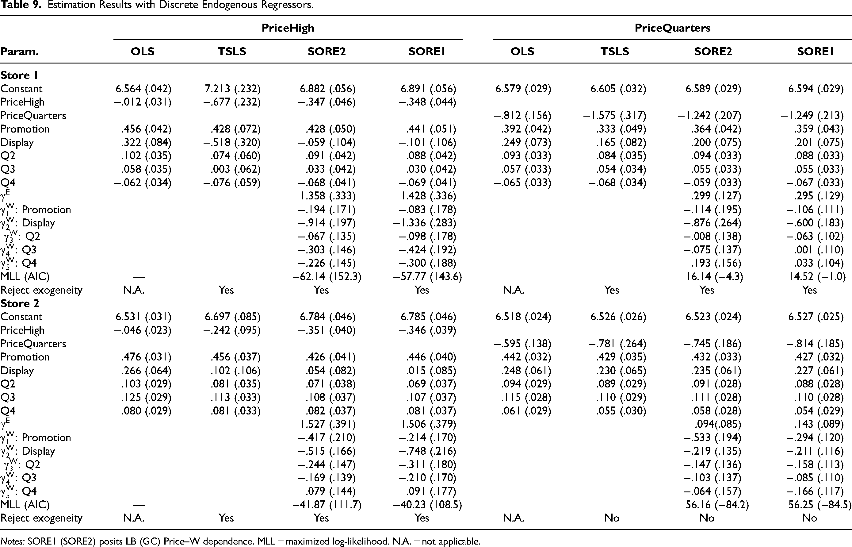
Notes: SORE1 (SORE2) posits LB (GC) Price–W dependence. MLL = maximized log-likelihood. N.A. = not applicable.

For Store 1, the estimates (standard errors) for PriceQuarters from OLS, TSLS, SORE2, and SORE1 are −.812 (.156), −1.575 (.317), −1.242 (.207), and −1.249 (.213), respectively (Table 9). We similarly find that the OLS price estimate has substantial upward bias and is outside of the 95% CI of the TSLS price estimate: −1.575 ± 1.96 × .317 = (−2.20, −.95). SORE can detect price endogeneity and yield a price estimate reasonably close to the TSLS estimate and within its 95% CI. Furthermore, the SORE price estimate has a smaller standard error than TSLS, due to the weaker IV used.

In Store 2, SORE1 and SORE2 yield almost identical AICs and similar price coefficient estimates. Compared with Store 1, price coefficient estimates from TSLS and SORE are even closer to each other, supporting the validity of the SORE estimates. Furthermore, Hausman tests for endogeneity using TSLS confirms that PriceHigh is endogenous (p < .01), but PriceQuarters is not (p > .01) in Store 2. SORE1 (SORE2 is similar) produces similar endogeneity test results: p < .001( ${\mathrm{Z}}_{{\gamma }^{\mathrm{E}}}=\frac{1.506}{.379}=3.9$ ) for PriceHigh, and p > .1 ( ${\mathrm{Z}}_{{\gamma }^{\mathrm{E}}}=\frac{.143}{.089}=1.61$ ) for PriceQuarters in Store 2.

Conclusion

Proper study design and best data collection (including observable instruments) should always be considered first for causal inference before resorting to poststudy estimation methods. However, ideal study design or data collection frequently is not achievable (e.g., for ethical reasons, poor external validity of experiments, lack of good IVs). Given the challenges in implementing ideal study designs and identifying valid IVs to control for endogeneity bias, developing feasible IV-free bias-correction methods is a viable and attractive alternative, when no ideal study designs or good IVs are available.

We propose a novel IV-free joint estimation approach to correcting for endogeneity bias due to regressor–error dependence. The approach employs flexible SORE models for the conditional distribution of endogenous regressors given the structural error and exogenous regressors, and obtains all parameter estimates in one step by maximizing the joint likelihood of endogenous regressors and structural error given exogenous regressors. ¹⁵

The empirical application illustrates that SORE either handles situations that existing IV-free methods cannot deal with or provides opportunities to improve the accuracy of causal effect estimation, and can be useful in several ways. First, empirical researchers can use SORE to handle discrete endogenous regressors more effectively. The application to the paper towel data shows that SORE yields plausible price coefficient estimates when the pricing variable has only a few levels (Table 9), demonstrating the unique capability of SORE to handle discrete endogenous regressors with few levels. Second, researchers can use SORE as a device to discover novel identification strategies. We derive a new identification strategy encoded by the LB OR function and illustrate its use in the application. We envision that more novel identification strategies will be motivated and discovered in the SORE framework. Last, SORE can be used as a multimethod approach to improve the robustness and quality of causal inference (Papies, Ebbes, and Feit 2022). The development of SORE moves toward this goal by nesting JCM in a more general framework that permits both copula and noncopula regressor–error dependence. Robustness of causal estimation can be assessed by comparing results from OR functions supported by theoretical considerations or selected by model selection measures. In the paper towel application, comparisons of different OR functions using AIC find some evidence favoring the LB regressor–error dependence (Table 7). Both TSLS and the best SORE model (M1) assuming the LB regressor–error dependence selected by AIC yield 95% CIs that exclude the OLS price estimate in Store 1, whereas that from the best SORE model (M2) assuming GC regressor–error dependence does not (Table 8). Despite these numerical differences, the price estimates from the two selected SORE models in Store 1 are both reasonably close to the TSLS price estimate. Furthermore, the TSLS, two selected SORE models, and JCM all (1) find price endogeneity and yield price estimates showing greater price sensitivity than the OLS price estimate in Store 1, and (2) find no price endogeneity in Store 2, ¹⁶ demonstrating the robustness to the assumed regressor–error dependence structures.

SORE has notable limitations and avenues for future research. SORE requires nonnormally distributed endogenous regressors for model identification. Despite the use of profile likelihood to eliminate nuisance parameters, SORE for continuous endogenous regressors can demand considerable computation time. For continuous endogenous regressors, it is straightforward to implement with minimal computation time the generated regressor copula endogeneity correction approach (Park and Gupta 2012) and the two-stage generated regressor copula approach (Yang, Qian, and Xie 2022). The latter approach is also able to handle normally distributed endogenous regressors. The proposed likelihood-based model selection to compare different OR functions does not incorporate prior beliefs. Bayesian approaches can be more suitable for this purpose as well as for handling large parameter spaces and weak model identification problems. This work considered two broadly applicable dependence structures: GC and LB. Studying new classes of OR functions could expand the applicability and capability of SORE. Finally, extending SORE to panel data is an important research avenue.

Supplemental Material

sj-pdf-1-mrj-10.1177_00222437231195577 - Supplemental material for Correcting Regressor-Endogeneity Bias via Instrument-Free Joint Estimation Using Semiparametric Odds Ratio Models

Supplemental material, sj-pdf-1-mrj-10.1177_00222437231195577 for Correcting Regressor-Endogeneity Bias via Instrument-Free Joint Estimation Using Semiparametric Odds Ratio Models by Yi Qian and Hui Xie in Journal of Marketing Research