Sage Journals: Discover world-class research

Abstract

The authors propose a new truth-telling technique and statistical model called “item count response technique” (ICRT) to assess the prevalence and drivers of sensitive consumer behavior. Monte Carlo simulations and a large-scale application to self-reported cigarette consumption among pregnant women (n = 1,315) demonstrate the effectiveness of the procedure. The ICRT provides more valid and precise prevalence estimates and is more efficient than direct self-reports and previous item count techniques. It accomplishes this by (1) incentivizing participants to provide truthful answers, (2) accounting for procedural nonadherence and differential list functioning, and (3) obviating the need for a control group. The ICRT also facilitates the use of multivariate regression analysis to relate the prevalence of the sensitive behavior to individual-level covariates for theory testing and policy analysis. The empirical application reveals a significant downward bias in prevalence estimates when questions about cigarette consumption were asked directly to pregnant women, or when standard item count techniques were used. The authors find lower smoking prevalence among women with higher levels of education and who are further along in their pregnancy, and a much higher prevalence among unmarried respondents.

Keywords

item count technique item response theory list experiment sensitive questions smoking

Marketing managers, policy makers, and researchers are often interested in assessing the prevalence and drivers of “dark side” and “vice” consumer behaviors, such as illegal movie streaming; software downloading; shoplifting; tax evasion; or consumption of prohibited drugs, pornographic material, alcohol, or tobacco (Andrews et al. 2004; De Jong, Pieters, and Fox 2010; Wang, Lewis, and Singh 2016; Weaver and Prelec 2013). Because of the sensitive and sometimes unlawful nature of such behaviors, consumers may not respond truthfully to direct questions about them even when they are common. The resulting response bias hinders identification of the true prevalence of the behaviors in the target population and impedes effective managerial decision making and policy evaluation.

We propose a new truth-telling technique to assess the prevalence and drivers of such sensitive consumer behavior. Our methodology builds on the item count technique (ICT) to administer sensitive questions in surveys. Rather than asking consumers to respond to a sensitive question in isolation, the ICT asks consumers to count the number of affirmative responses to a set of items that includes the sensitive question. The added privacy protection increases truthful responding. Despite its intuitive appeal and growing usage in other disciplines (Coffman, Coffman, and Marzilli Ericson 2017; Imai 2011; Kuha and Jackson 2014; Nepusz et al. 2014),¹ the ICT has not yet been applied in marketing. Moreover, existing applications of the technique have important shortcomings that prevent it from reaching its full potential. We propose the “item count response technique” (ICRT) to address these issues. Our research fits in a larger stream of marketing research on truth-telling for stated preference data, such as randomized response and similar techniques for surveys (De Jong, Pieters, and Fox 2010; Weaver and Prelec 2013), incentive alignment in conjoint settings (Ding, Grewal, and Liechty 2005), and behavioral research on when consumers are willing to divulge sensitive information (John, Acquisti, and Loewenstein 2011).

The proposed ICRT is applicable to a variety of sensitive consumer behaviors. It comprises a data collection method and a statistical model to make inferences about the prevalence of the sensitive behavior and its correlates. We demonstrate the potential effectiveness of the ICRT using Monte Carlo simulations and apply it in the context of a very sensitive behavior: cigarette consumption during pregnancy (Bradford 2003). Smoking during pregnancy puts not only the prospective mothers but also their unborn children at serious risk of contracting an alarming range of defects and inflictions (Hackshaw, Rodeck, and Boniface 2011), resulting in multimillion-dollar neonatal health care costs (Adams et al. 2002). The design and evaluation of countermarketing and antismoking programs rests on the accuracy of estimates of smoking prevalence and its correlates (Andrews et al. 2004; Wang, Lewis, and Singh 2016). However, the societal stigma about smoking, in particular smoking during pregnancy, may prevent prospective mothers from admitting their smoking habit and thus leading them to underreport their smoking status when answering direct questions in surveys (Dietz et al. 2011; Lumley et al. 2009). Using biomarkers to establish smoking prevalence among pregnant women is prohibitively costly and difficult to implement on a large scale. Thus, Jain (2017, p. 9) stresses in a comprehensive review that “efforts must be made to improve survey questionnaire content and/or methodology to be able to obtain better estimates of smoking prevalence.” Our research follows up on this call.

The next section presents the standard ICT and its assumptions. Then, we describe our new technique and how it improves on existing ones. We present Monte Carlo simulations to assess the performance of the new technique relative to standard techniques and our empirical application to cigarette smoking among pregnant women. We end with a discussion, suggestions for implementation of the procedure, and for recommendations for future research.

The ICT

The standard ICT uses a two-group design to ask sensitive questions. A sample of respondents is randomly assigned to either a control group or a treatment group. Respondents in the control group receive a list of baseline questions. Respondents in the treatment group receive the same list of baseline questions plus one extra question: the target item. The ICT is an indirect self-report technique—that is, respondents in both groups do not have to indicate directly whether they affirm or disconfirm each individual item in their list. Instead, they only have to count and report the total number of items in their list that they affirm. Then, the prevalence estimate of the target item is derived by taking the difference in the average number of affirmative responses between the treatment and control group. In an early application, Kuklinksi, Cobb, and Gilens (1997) asked respondents how many from a list of three (control group) or four (treatment group) events would anger or upset them, with the fourth, target event being, “A black family moving in next door.” For respondents in the U.S. South, the average item counts were, respectively, 1.95 in the control group and 2.37 in the treatment group, implying that such an event would anger or upset 42% of respondents in the treatment group (2.37 − 1.95 = .42). The ICT protects the privacy of respondents in the treatment group because it is impossible to determine what a respondent’s answer to the target item would be. Table 1 summarizes the ICT and its assumptions and compares the standard implementation (first column: type A), which has been most widely used, with recent improvements.

Table 1.

ICT: Characteristics and Assumptions.

Type	Design	Identification Strategy	Analysis Level	Assumptions			Representative Studies
Type	Design	Identification Strategy	Analysis Level	Group Equivalence	Procedural Adherence	Homogeneous List Functioning	Representative Studies
A	Multiple samples	Difference in means of groups (samples)	Group	Tested	Assumed	Assumed	Anderson et al. (2007); Corstange (2009), Glynn (2013), Kuklinski, Cobb, and Gilens (1997)
B	Single sample	Known group-level prevalence of baseline items	Group	Redundant	Assumed	Assumed	Nepusz et al. (2014), Petróczi et al. (2011)
C	Multiple samples	Estimated probability of (sum of) baseline items	Individual	Tested	Tested	Tested	Blair and Imai (2012), Imai (2011), Imai, Park, and Greene (2015), Kuha and Jackson (2014)
D	Single sample	Estimated probability of each “inside” baseline item from “outside” baseline items	Individual	Redundant	Accounted	Accounted	This research

Notes: The basic data collection design requires at least two samples, namely, a treatment and a control group. Some applications (e.g., Anderson et al. 2007; Blair and Imai 2012) use multiple treatment groups with different target items. “Identification Strategy” describes how the prevalence (group level) or probability (individual level) of the target item is inferred from the list sum reported by respondents.

Compared with direct questioning (DQ), the ICT increases the willingness of respondents to truthfully disclose sensitive information. This finding is consistent across multiple versions of the ICT and across a variety of attitudes and behaviors, such as racial and gender attitudes (Imai 2011; Kuklinski, Cobb, and Gilens 1997), election attitudes and behavior (Corstange 2009; Imai, Park, and Greene 2015), eating-disordered behaviors (Anderson et al. 2007), recreational drug use (Nepusz et al. 2014), high-risk sexual behavior (Tian et al. 2014), and various forms of delinquency (Wolter and Laier 2014).

The ICT has several strengths compared with other self-report techniques that aim to elicit truthful answers, such as the randomized response technique (RRT) (De Jong, Pieters, and Fox 2010; Fox, Avetisyan, and Van der Palen 2013; Lamb and Stern 1978). In the RRT, the sensitive question is asked directly, but a randomization mechanism adds “noise” to the respondent’s answer. Thus, the researcher does not know whether the answer that a respondent provides is true or forced by the randomization device. For example, respondents might be asked whether they currently smoke or not. They are instructed to provide their true answer when a real or electronic coin comes up heads, and to respond with a forced “yes” when the coin comes up tails. Because the probability of the forced “yes” is known from the randomization device, prevalence of the sensitive behavior at the sample level can be readily inferred.

An important strength of the ICT relative to the RRT is that the instructions to respondents are generally easier to understand, which reduces measurement error from miscomprehension. A second strength is that the ICT does not rely on a randomization device, which increases the trustworthiness of the privacy protection and thereby adherence to the data collection procedure. Moreover, the ICT does not force respondents to select a particular answer that they do not like, which also increases adherence to the procedure. Together, this makes the ICT well-suited to be used in large-scale self-administered surveys for marketing research and policy purposes.

Identification Strategy and Assumptions of the ICT

The standard ICT uses the difference in the mean reported list sums between the treatment and control group to identify the prevalence of the target item (Table 1, type A). That is, the treatment group (T) receives a list of K baseline items plus the target item. The probability of an affirmative response for respondent i on baseline item k (k = 1,…, K) then is

Pr (Z_{i k}^{(T)} = 1) = p_{k}^{(T)},

where $Z_{i k}^{(T)}$ is a Bernoulli random variable. Note that $p_{k}^{(T)}$ is not individual-specific and that the random variable $Z_{i k}^{(T)}$ is latent because only the list sum is observed. The list sum for a respondent i in the treatment group is then

Y_{i}^{(T)} = \sum_{k = 1}^{K} Z_{i k}^{(T)} + U_{i},

where U_i is the binary response to the target item. In the control group (C), respondents receive a list with only the K baseline items. In that group, for k = 1,…, K, the probability of an affirmative response for respondent j and the list sum is

Pr (Z_{j k}^{(C)} = 1) = p_{k}^{(C)}, and

Y_{j}^{(C)} = \sum_{k = 1}^{K} Z_{j k}^{(C)} .

The prevalence of the target item then is calculated as the difference in means between groups:

{\overset{○}{p}}_{K + 1} = \frac{1}{N_{T}} \sum_{i = 1}^{N_{T}} Y_{i}^{(T)} - \frac{1}{N_{C}} \sum_{j = 1}^{N_{C}} Y_{j}^{(C)},

where N_T is the number of respondents in the treatment group, and N_C is the number of respondents in the control group. Importantly, three assumptions need to be met to estimate the prevalence of the sensitive behavior consistently and unbiasedly from Equation 5:

Group equivalence: Respondents in the treatment and control groups are equivalent in all characteristics, except in the content of the item list they receive.

Procedural adherence: Respondents adhere to the instructions and truthfully answer the target item. Then, $U_{i} = U_{i}^{*}$ , where $U_{i}^{*}$ is the truthful answer to the target item.

Homogenous list functioning: The target item in the list does not change the sum of affirmative answers to the K baseline items. That is, the sum of the Z_ik, k = 1,…, K are the same no matter whether respondent i is in the treatment group or control group.

Assumption 1 is met by random assignment of respondents to treatment and control group and violated without it. Assumption 2 is likely to be violated when there is a ceiling effect (Corstange 2009). A ceiling effect occurs when truthful answers require a respondent to answer all items in the list affirmatively: $Y_{i}^{(T)} = K + 1$ . Yet then the researcher would know that the response to the target item is affirmative, which violates respondents’ privacy protection. To prevent this, some respondents can choose to provide a nontruthful answer to the target item, so that the reported item count becomes K instead of K + 1. Even with careful list design (Corstange 2009), ceiling effects are likely to occur for some respondents, with nonadherence as a consequence. Assumption 3 is also violated when the sensitivity, salience, or “weirdness” of the target item relative to the more neutral, baseline items biases respondents’ comprehension and judgment and, thus, their response to the baseline items (Kuha and Jackson 2014; Tourangeau and Yan 2007). Importantly, violating Assumptions 2 or 3 also violates Assumption 1, because then treatment and control groups differ in more than the mere content of their lists.

While simple to implement and analyze, the standard ICT has three major drawbacks that may hamper its validity and widespread application in theory testing and policy application. First, it can neither test nor account for cases that its assumptions are violated, resulting in unknown, biased estimates. Second, it makes inefficient use of the available sample size, because only the treatment group answers the sensitive item. Third, it provides prevalence estimates of the sensitive behavior at the group level rather than at the individual level, which impedes theory testing and targeted policy making (Table 1: “Analysis Level” column).

Assumption tests

To address the first issue, Imai (2011) and Blair and Imai (2012) propose formal tests of Assumptions 2 and 3 (Table 1: type C). However, as yet there are no principled approaches to cope with situations that the assumptions are violated.

Single sample approach

To address the second issue, Nepusz et al. (2014) propose the “single sample item count technique,” which uses a single sample of respondents only. Then, all respondents receive a list with the target item and baseline items. To identify the prevalence of the target item, baseline items are used that each have a known 50/50 probability in the population of interest (Table 1: Type B). Examples of such baseline items are whether a respondent has a birthday that falls on an even or uneven day, was born in the first or the last six months of the year, is male or female, or lives at an address with even or uneven street number (Nepusz et al. 2014; Petróczi et al. 2011). The proportion of respondents affirming the target item can then be readily estimated, as the average response percentage above the known joint baseline item percentage. There are several limitations of this approach. First, using evidently uninformative baseline items makes the sensitive, target item salient, and adds to the “weirdness” of the overall list (Kuha and Jackson 2014, pp. 12–13). This increases the likelihood of procedural nonadherence and differential list functioning, violating Assumptions 2 and 3. Second, the approach makes it virtually impossible to examine the impact of individual-level drivers of the target behavior, because the distributions of the baseline items are only known at the population level.

Individual-level analysis

To enable inferences about individual-level drivers of the target behavior, Imai and colleagues (Imai 2011; Imai, Park, and Greene 2015) generalize the difference-in-means estimator in Equation 5. Collecting all list scores in the vector Y (that is, $Y = (Y_{1}^{(T)}, \dots, Y_{N_{T}}^{(T)}, Y_{1}^{(C)}, \dots, Y_{N_{C}}^{(C)})$ , they formulate the following regression model:

Y_{i} = X_{i} γ + T_{i} X_{i} γ + ∊_{i} .

Such a specification implies that X_iγ captures the effect of the covariates in X_i on the list score of respondents in the control group. Yet, because baseline items in the list are often weakly or even uncorrelated, the variance accounted for by the covariates in X_i will tend to be low. Thus, estimates of the probability that respondent i affirms the target item are likely to be imprecise and difficult to estimate. As a case in point, Wolter and Laier (2014) using the provided R program could not get the Imai estimator to converge in their application.

Kuha and Jackson (2014) go one step further by estimating the probability of affirming each of the baseline items, through a set of explanatory variables for each of the Z_ik. Yet, their model assumes that the relationship between predictors and baseline items is invariant across treatment and control groups (assumption 3), and the prevalence estimates are sensitive to the exact model assumed for the baseline items (idem, p. 335). That is, both the distribution assumed for the Z_ik, and the specific explanatory variables (and possible interactions) included in the model for the Z_ik affect the prevalence estimates, which is undesirable.

The ICRT Methodology

The ICRT methodology improves on previous techniques in three important ways (Table 1, type D). First, it uses a single sample only. This makes Assumption 1 redundant and uses survey resources efficiently. Second, it accounts for situations in which Assumptions 2 and 3 are violated. This provides valid estimates of the sensitive behavior even in cases of procedural nonadherence and differential list functioning. Third, it uses information provided by (and known only to) respondents elsewhere in the survey to accurately estimate the probability of affirming each of the baseline items in the list. This enables estimating the probability of the sensitive behavior at the individual level and facilitates multivariate analyses of potential correlates of the target behavior. Let us describe data collection and statistical model of ICRT.

Data Collection

Our identification strategy is to make use of the correlation between baseline items “inside” the list and baseline items “outside” the list elsewhere in the questionnaire. This correlation allows us to estimate the probability that each of the baseline items inside the list is affirmed. From that information, we can identify the probability that the target item in the list is affirmed at the individual level using a single sample of respondents only.

Specifically, we propose to use K baseline items inside the list that come from K different validated multi-item measures of latent variables, such as attitudes or traits (Bearden, Netemeyer, and Haws 2011). For now, assume that these K baseline items are unrelated to the target item in the list (we relax this assumption later). One item from each of the K measures is included as a baseline item inside the list. Assume that measure k consists of N_k items that reflect a latent variable (θ_ik). Because one of its items is already inside the list, N_k − 1 items remain in measure k. These remaining items are administered outside the list, before or after, and are asked directly. These “outside” baseline items may be measured on a binary or polytomous response scale.

To illustrate, consider the data collection in our empirical application. Respondents first answer a few baseline items directly. Baseline items are based on the impulsiveness and self-discipline facets (two items from each) of the Big Five personality trait inventory (Costa and McCrae 2008), and are shown in a matrix table:

	Strongly Disagree	Disagree	Neither Agree Nor Disagree	Agree	Strongly Agree
1. When I am having my favorite foods, I tend to eat too much.	○	○	○	○	○
2. I have trouble resisting my cravings.	○	○	○	○	○
3. I have no trouble making myself do what I should.	○	○	○	○	○
4. When a project gets very difficult, I never give up.	○	○	○	○	○

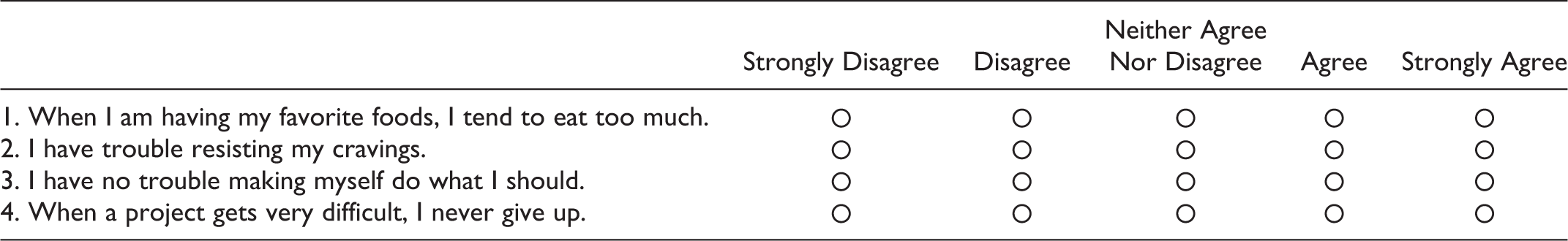
Later in the questionnaire, the list section is introduced as follows:

Below, you will find three statements. We would like to know HOW MANY of these statements are true (we do not wish to know which statements are true or false, only how many are true).

I currently smoke at least 1 cigarette per day.

Sometimes I do things on impulse that I later regret.

I’m pretty good about pacing myself so as to get things done on time.

Inside this list, item (a) is the target item, item (b) measures impulsiveness, and item (c) measures self-discipline. Thus, baseline items 1 and 2 outside the list and baseline item (b) inside the list all measure impulsiveness (Hyman 2001, p. 127). Because a latent trait (θ_{i, impulsiveness}) underlies responses to all three items, these should be strongly correlated. Knowing the answer to baseline items 1 and 2 outside the list then enables predicting the answer to the baseline item (b) inside the list, even though we do not observe the answer to that item in the data. The same reasoning holds for baseline items 3 and 4 outside the list and baseline item (c) inside the list.

To formalize the reasoning, because item k in the list comes from validated measure k, it is natural to assume that

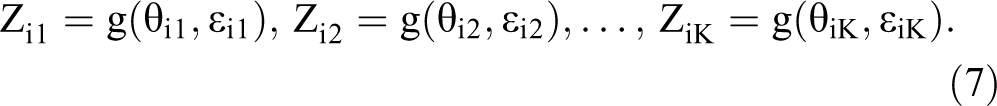
Z_{i 1}^{} = g (θ_{i 1}, ∊_{i 1}), Z_{i 2}^{} = g (θ_{i 2}, ∊_{i 2}), \dots, Z_{i K}^{} = g (θ_{i K}, ∊_{i K}) .

That is, the unobserved baseline item Z_ik inside the list is a function of the latent variable score θ_ik and of unique variance captured in ∊_ik. The high intercorrelations between items from validated measures enable estimating Z_ik in the list using information from baseline items assessed directly, outside the list.²

Statistical Model

We use an item response theory (IRT) specification to estimate the response to the target item in the list, given the total item count from the list and the responses to the baseline items outside the list. Thus, the name “item count response technique.” To specify the functions g(.) in Equation 7, assume a total of H polytomous baseline items administered outside the list, where $H = \sum_{k} (N_{k} - 1)$ and k(h) indicates the baseline latent variable measured by item h. The observed score $X_{i h}^{(θ)}$ on item h, h = 1,…, H can then be modeled as

Pr (X_{i h}^{(θ)} = c | θ_{i, k (h)}, a_{h}, γ_{h}) = Φ [a_{h} (θ_{i, k (h)} - γ_{h, c - 1})] - Φ [a_{h} (θ_{i, k (h)} - γ_{h, c})] .

This model specifies the conditional probability of a respondent i, responding in a category c (c = 1,…, C) for item h, as the probability of responding above c − 1, minus the probability of responding above c. The specification is a graded-response IRT model (Samejima 1969), with latent variable θ_{i, k(h)}, discrimination parameter a_h and threshold parameters γ_h,1 <…< γ_{h, C}. Discrimination parameters are conceptually similar to factor loadings in a factor-analytic framework. The threshold γ_{h, c} is the value on the scale of θ_{i, k(h)}, where the probability of responding above a value c is .5.

Next, we focus on the list-based items. Because the list contains K baseline items from existing multi-item measures, we modify Equation 1 using the two-parameter normal ogive IRT model. Thus, for k = 1,…, K:

p_{i k}^{} = Pr (Z_{i k}^{} = 1 | θ_{i k}, a_{l i s t, k}^{}, b_{l i s t, k}^{}) = Φ (a_{l i s t, k}^{} θ_{i k} - b_{l i s t, k}^{}),

with $(θ_{i 1}, \dots, θ_{i K}) \sim M V N (μ, Σ)$ . Here, the value Z_ik depends on the individual-specific value of latent variable θ_ik, item parameters (discrimination a_{list, k} and difficulty b_{list, k}) and random error. The interpretation of the discrimination parameter a_{list, k} is the same as in Equation 8. The difficulty parameter b_{list, k} captures how “easy” it is for respondents to answer affirmatively to item k. For the target item K + 1, we posit:

p_{K + 1} = Pr (U_{i} = 1) .

An attractive feature of the specification in Equations 8 through 10 is that it is sufficient to derive the probability of an observed item count Y_i for the list. For instance, with two baseline items and one target item inside the list, and a corresponding item count that ranges between 0 and 3, because of conditional independence we have:

Pr (Y_{i} = 0) = (1 - p_{i, 1}) (1 - p_{i, 2}) (1 - p_{K + 1}),

Pr (Y_{i} = 1) = p_{i, 1} (1 - p_{i, 2}) (1 - p_{K + 1}) + (1 - p_{i, 1}) p_{i, 2} (1 - p_{K + 1}) + (1 - p_{i, 1}) (1 - p_{i, 2}) p_{K + 1},

Pr (Y_{i} = 2) = p_{i, 1} p_{i, 2} (1 - p_{K + 1}) + p_{i, 1} (1 - p_{i, 2}) p_{K + 1} + (1 - p_{i, 1}) p_{i, 2} p_{K + 1}, and

Pr (Y_{i} = 3) = p_{i, 1} p_{i, 2} p_{K + 1} .

So far, we assumed that the baseline items are unrelated to the target item in the list, as in prior ICT research (Glynn 2013; Imai 2011; Kuha and Jackson 2014; Nepusz et al. 2014; Tian et al. 2014). Our model can relax this assumption. It models the potential association between the baseline traits and the target behavior now indexed by i, via a standard Probit regression:

p_{i, K + 1} = Pr (U_{i} = 1) = Φ (β_{0} + {β'}_{1} θ_{i} + β_{2} X_{i}),

where X _i contains individual-level covariates. Our approach thus probabilistically infers the response to the sensitive item, and the true response to the sensitive item is therefore not known (except in case of a ceiling response). Note that if the baseline items are uncorrelated with the sensitive item, β ₁ = 0. Our model allows the traits reflected in the baseline items, together with socioeconomic and other personal characteristics of the respondents to predict the prevalence of the target behavior. When using Equation 15, Equations 11 through 14 remain the same, but the parameter p_{K + 1} becomes p_{i, K + 1}.

Accounting for Assumptions

Because the ICRT requires a single sample only, Assumptions 1 and 3 concerning group equivalence and homogeneous list functioning are redundant.

To account for nonadherence due to ceiling, we model an intermediate step in the response process in which respondents may decide to “edit” their true answer if their true list score equals K + 1. Denoting the true list score by ${\tilde{Y}}_{i}$ , we therefore specify the probability of nonadherence (τ) as

Pr (Y_{i} = K | {\tilde{Y}}_{i} = K + 1) = τ .

Then the probabilities of answering K + 1 and answering K become, respectively,

Pr (Y_{i} = K + 1) = (1 - τ) Pr ({\tilde{Y}}_{i} = K + 1), and

Pr (Y_{i} = K) = τ Pr ({\tilde{Y}}_{i} = K + 1) + Pr ({\tilde{Y}}_{i} = K) .

These altered list score probabilities can be substituted in the likelihood function.

Model Estimation

Estimation of the proposed model is challenging because of its high dimensionality. While some researchers have relied on expectation–maximization algorithms to estimate previous item count models (Blair and Imai 2012, Imai 2011; Tian et al. 2014), the multidimensional integrals required here make an expectation–maximization algorithm cumbersome to implement. Therefore, we rely on Markov chain Monte Carlo (MCMC) methods (Bradlow, Wainer, and Wang 1999; Fox and Glas 2001; Rossi, Allenby, and McCulloch 2005). The likelihood for the ICRT is

L ({a_{h}, γ_{h}}, {a_{l i s t, k}, b_{l i s t, k}}, μ, Σ, τ | X^{(θ)}, Y) = \prod_{i = 1}^{N} \int [\prod_{h = 1}^{H} \prod_{c = 1}^{C} Pr {(X_{i h}^{(θ)} = c | θ_{i}, a_{h}, γ_{h})}^{I (X_{i h}^{(θ{)} = c)}] \times Pr {(Y_{i} = K + 1 | θ_{i}, a_{list}, b_{list})}^{I (Y_{i} = K + 1)} \prod_{k = 1}^{K} Pr {(Y_{i} = k | θ_{i}, a_{l i s t}, b_{l i s t})}^{I (Y_{i} = k)} f (θ_{i} | μ, Σ) d θ_{i} .

To identify the latent variables θ _I, we fix the mean μ to a zero vector and specify the variance–covariance matrix Σ as a correlation matrix, with diagonal elements equal to 1. A full probability model is required for model estimation. We use a data augmentation step (Tanner and Wong 1987) to simulate for each respondent the values of Z_ik and U_i. To do so, we compute the following:

Pr (Z_{i 1} = z_{i 1}, \dots, Z_{i K} = z_{i K}, U_{i} = u_{i} | Y_{i} = k),

after which we can simultaneously draw {Z_i1,…, Z_iK, U_i} using the probabilities in Equation 20. Note that two particularly easy cases are when Y_i = 0, implying that U_i = 0, or when Y_i = K + 1, implying that U_i = 1. Estimation details are in Web Appendix 1. We used MATLAB to estimate all models. The Web Appendix provides WinBUGS code (Spiegelhalter et al. 1996) to facilitate wider adoption of the method.

We compare the observed list score distribution to replicated list score distributions from the posterior predictive distribution:

p (Y_{i}^{r e p} | Y_{i}) = \int p (Y_{i}^{r e p} | Y_{i}, ω) p (ω | Y_{i}) d ω,

with $p (ω | Y_{i})$ representing the posterior of all parameters in the model, and which uses Equations 12 through 15 to predict Y_i. If the model fits the data well, the frequency distribution of the replicated data (i.e., the number of observed 0, 1, 2,…, K + 1 responses) should be similar to the frequency distributions of the observed list data.

In addition, we test the importance of model components (such as the need to include a nonadherence parameter) using the pseudo-Bayes factor (Geisser and Eddy 1979; see also Web Appendix 1). Values of the pseudo-Bayes factor closer to zero indicate better fit.

Monte Carlo Simulation

We conducted two Monte Carlo simulation studies that compare the performance of the proposed ICRT with the standard ICT estimator under a range of conditions. We describe these studies in the following subsections.

Differential List Functioning, Nonadherence, and Correlation with Baseline Traits

Study 1 assesses the violation of which assumptions threatens the validity of the standard ICT most. It also demonstrates that the ICRT can then still recover the true proportions. The experimental design has 20 conditions, namely 4 (assumption: differential list functioning of difficulty, and of discrimination parameters, procedural nonadherence, and correlation between baseline trait and target item) × 5 (true proportion of target item: .10, .30, .50, .70, and .90), each with 20 replication data sets. True sensitive proportions can vary widely.³ In their review, Wolter and Preisendorfer (2013) document proportions of the sensitive behavior varying from 19% to 100%. Therefore, our simulations consider a wide range of proportions as well.

Each data set has 2,000 respondents in the list group and 2,000 respondents in a control group who receive DQ. The control group is needed for the standard ICT estimator, but not for the ICRT estimator. For each data set, we compute the prevalence estimates of the target behavior for the standard ICT and for the ICRT estimator using 5,000 burn-in draws and 5,000 draws for posterior inference for each replication data set.

The item list has two baseline items and a target item. The two baseline items are generated according to an IRT model, with discrimination and difficulty parameters specified in Table 2. Furthermore, for the ICRT model, there are H = 6 baseline items outside the list, each item measured on a five-point response scale. The first (last) three outside baseline items and the first (second) inside baseline item measure the same latent trait. Web Appendix 2 has details about item parameters. Item parameters are chosen such that the reliabilities of baseline trait are .80, in line with typical reliabilities of validated scales (Bearden, Netemeyer, and Haws 2011).

Table 2.

Simulation Study 1: Performance of ICT and ICRT Under Differential List Functioning, Nonadherence, and Trait-Target Correlation.

True Proportion	Differential List Functioning				C: Procedural Nonadherence		D: Correlation Baseline Traits and Sensitive Item
	A: Difficulty Parameters		B: Discrimination Parameters		C: Procedural Nonadherence		D: Correlation Baseline Traits and Sensitive Item
	ICT	ICRT	ICT	ICRT	ICT	ICRT	ICT	ICRT
.10	−.36	.11	.12	.10	.09	.09	.10	.10
.30	−.16	.30	.32	.29	.27	.30	.28	.30
.50	.05	.50	.52	.51	.44	.50	.46	.49
.70	.25	.70	.72	.70	.61	.70	.63	.70
.90	.44	.90	.92	.89	.79	.90	.79	.90

Notes: a = item discrimination; b = item difficulty; τ = incidence of procedural nonadherence. For Panel A: a_{1, list} = a_{1, DQ} = 1.1, a_{2, List} = a_{2, DQ} =1.2, and b_{1, list} = .1, b_{1, DQ} = −.9, b_{2, list} = .3, b_{1, DQ} = −.5. For Panel B: a_{1, list} = .5, a_{1, DQ} = 1.1, a_{2, list} = .8, a_{2, DQ} = 1.2, and b_{1, list} = b_{1, DQ} = −1, b_{2, list} = b_{1, DQ} = 1. For Panel C: a_{1, list} = a_{1, DQ} = 1.1, a_{2, list} = a_{2, DQ} =1.2, and b_{1, list} = b_{1, DQ} = .1, b_{2, list} = b_{1, DQ} = .3, and τ =.6. For Panel D: a_{1, list} = a_{1, DQ} = a_{2, list} = a_{2, DQ} =1.4, and b_{1, list} = b_{1, DQ} = −.5, b_{2, list} = b_{1, DQ} = .3, τ =.5, and $β_{1} = - .6, β_{2} = - .5$ . Moreover, for Panel D nonadherence is set at 50% and $p_{i, K + 1} = Φ (β_{0} + β_{1} θ_{i 1} + β_{2} θ_{i 2})$ , with β₁ = −.6, β₂ = −.5, and β₀ across conditions such that the average probability of affirming target item ${\bar{p}}_{K + 1}$ is .10, .30, .50, .70, and .90, depending on condition. Mean prevalence estimates shown across 20 replication samples for each condition.

Table 2 reports the average ICT and ICRT estimates across the 20 replication data sets for each of the conditions. Panels A and B report the impact of differential list functioning (difficulty and discrimination parameters) on model performance. Panel C reports the impact of procedural nonadherence, and Panel D reports the impact of correlation between the baseline traits and the target item in the list on model performance.

Across conditions, the standard ICT underestimates the true proportion by 44% on average, whereas the ICRT underestimates the true proportion by .1% only (difference t(798) = 8.48, p < .001). Differential item difficulty (Panel A) can produce severe underestimates up to 460% of the true prevalence for the standard ICT (average underestimation 163%) but leaves ICRT estimates essentially unharmed (average overestimation 1.7%, t(198) = 10.88, p < .001). Differential discrimination parameters (Panel B) produce an average overestimation of 7.4% for the standard ICT (7.4%), and less than 1% underestimation for ICRT (difference t(198) = −5.04, p < .001). The large difference in bias for ICT due to differential difficulty versus differential discrimination parameters is because a shift in difficulties directly shifts the argument of the standard normal cdf (Equation 9), whereas the discrimination only shifts the argument of the standard normal cdf indirectly through multiplication by theta. Because theta has a mean of zero, the impact of the discrimination parameter will be smaller. Even procedural nonadherence of 60% (Panel C) leaves ICRT estimates essentially intact (<1% underestimation) but biases standard ICT estimates downward up to 30% (average underestimation 12.6%, difference t(198) = 7.47, p < .001). Finally, correlation between baseline traits and target item (Panel D) also leaves the ICRT estimates intact (<1% underestimation) but biases ICT estimates downward up to 12% (average underestimation 7.2%, difference t(198) = 4.07, p < .001). Further meta-regressions support the large bias in prevalence estimates when using the standard ICT, and the improved accuracy and close to zero bias (<2%) when using the ICRT estimator, for all conditions (Web Appendix 2: Table WA4).

List Size and Reliability of Measures of Baseline Traits

Study 2 tests the effect of list size, reliability of baseline measures, differential list functioning, and procedural nonadherence in more detail for the following two reasons. First, larger list sizes improve the respondent’s privacy protection but also muddle the analyst’s task by exponentially increasing the number of possible response patterns that produce a specific list score. In typical applications of the ICT, the list size varies between three and five items. For a list size of three, only three response patterns produce a list score of two (Equation 13). Yet for a list size of five, already ten possible response patterns produce a list score of two. The large number of patterns impedes empirical identification, despite theoretical identification.

Second, a higher reliability of the multi-item measures of baseline traits increases precision of estimating the sensitive proportion. Because of their higher intercorrelations, the outside baseline items predict the inside baseline items better, which in turn improves estimating the response to the target item. Thus, higher reliability might offset reduced precision owing to larger list sizes.

The experimental design has 90 conditions, namely 3 (list size: three, four, or five items) × 3 (reliability of measures: .70, .80, and .90) × 2 (assumption: differential list functioning, or differential list functioning plus procedural nonadherence) × 5 (true proportion of target item: .10, .30, .50, .70, and .90), each with 20 replication data sets. As in Study 1, we report the means of 20 replication data sets. We use difficulty parameters for inside baseline items that produce about a .5 probability of an affirmative response. We introduce either mild differential list functioning or mild differential list functioning plus procedural nonadherence (details in Web Appendix 2) and establish how the ICT and ICRT estimators perform under these conditions. Table 3 summarizes the results.

Table 3.

Simulation Study 2: Performance of ICT and ICRT for Various List Sizes and Scale Reliabilities.

True Proportion	Reliability = .7				Reliability = .8				Reliability = .9
	DLF		DLF and PNA		DLF		DLF and PNA		DLF		DLF and PNA
	ICT	ICRT	ICT	ICRT	ICT	ICRT	ICT	ICRT	ICT	ICRT	ICT	ICRT
List size = three
.10	−.02	.10	−.04	.11	−.02	.10	−.03	.10	.03	.10	.01	.10
.30	.18	.31	.14	.30	.19	.31	.15	.30	.22	.30	.20	.30
.50	.37	.50	.30	.50	.39	.50	.31	.50	.42	.50	.37	.50
.70	.58	.70	.47	.70	.58	.70	.49	.70	.63	.70	.55	.70
.90	.78	.90	.65	.90	.79	.90	.66	.90	.83	.90	.72	.90
List size = four
.10	−.11	.11	−.11	.12	−.12	.10	−.12	.10	−.18	.10	−.20	.10
.30	.10	.32	.08	.30	.08	.31	.04	.29	.02	.30	−.01	.29
.50	.30	.52	.25	.51	.29	.51	.23	.50	.21	.50	.18	.50
.70	.51	.70	.42	.69	.49	.71	.40	.69	.42	.70	.37	.70
.90	.69	.89	.61	.88	.68	.90	.61	.89	.60	.90	.54	.90
List size = five
.10	−.13	.31	−.12	.33	−.12	.21	−.12	.24	−.10	.10	−.10	.10
.30	.08	.42	.08	.42	.08	.36	.07	.38	.10	.31	.11	.29
.50	.29	.51	.28	.50	.29	.50	.28	.52	.31	.51	.31	.51
.70	.48	.62	.47	.62	.49	.68	.46	.67	.50	.73	.51	.74
.90	.67	.86	.69	.88	.69	.90	.67	.90	.70	.92	.70	.91

Notes: DLF = differential list functioning; PNA = procedural nonadherence. Mean prevalence estimates are shown across 20 replication samples for each condition.

Across conditions, the standard ICT severely underestimates prevalence of the target item with on average 70%, whereas the ICRT overestimates this but much less at 10% on average (difference t(3,598) = 41.78, p < .001). Even at a moderate reliability of .70 and with a list size of three, the accuracy of the ICRT estimator is already very good, irrespective of the true proportion (Table 3, Column 1; average overestimation 1%). The standard ICT estimator performs much worse, with an average underestimation of 51%.

With larger list sizes, the standard ICT estimator progressively underestimates prevalence (underestimation at list sizes three, four, and five, respectively, is 44%, 89%, and 76%), while the ICRT estimator overestimates prevalence but much less (overestimation at list sizes three, four, and five, respectively, is <1%, 1%, and 27%). Importantly, and as predicted, when list size and reliability increase, the precision of the ICRT estimate increases as well (average bias < 1% at list size 5 and reliability of .90; see Table 3). Yet, the ICT estimator then still underestimates prevalence on average by 71%. At a list size of three, as in our empirical application, the ICRT estimator essentially has no bias (<1%) whereas the standard ICT estimator grossly underestimates prevalence (51%). Further metaregressions support the large bias in prevalence estimates for the standard ICT estimator and the improved accuracy for the ICRT estimator and show how improved reliability compensates bias from larger list sizes (Web Appendix 2; Table WA5).

Conclusion

The accuracy of the ICRT is very good, with essentially ignorable bias for list sizes of three and four at moderate levels of reliability of baseline trait measures. When the list size increases to five, high reliabilities of the baseline trait measures of .90 are needed to obtain reasonable prevalence estimates for the sensitive item, especially if the true sensitive proportion is low. Such high reliabilities require the use of conceptually and semantically very similar items, which is undesirable for reasons of privacy and trustworthiness. The “General Discussion” section returns to this topic.

The ICT and ICRT estimators perform equally well in case of full procedural adherence (Assumption 2) and homogenous list functioning (Assumption 3). Yet the ICRT but not the standard ICT estimator is shielded against bias when these assumptions are violated. For all examined conditions, the ICRT estimator outperforms the standard ICT estimator. The ICRT is also more efficient by leveraging the information contained in the baseline items outside and inside the list, even with small list sizes and at moderate levels of reliability of the baseline traits. The “General Discussion” section provides guidelines for the design of item count studies.

Empirical Application

The empirical application concerns cigarette consumption (“smoking”) by women during pregnancy. Large-scale research on cigarette consumption has typically relied on self-reports from population surveys, such as the National Health and Nutrition Examination Survey, the Global Adult Tobacco Survey, and the National Maternal and Infant Health Survey (Bradford 2003; Cui et al. 2014). The societal stigma that rests on smoking tobacco makes the validity of such self-reported smoking questionable, in particular for vulnerable segments such as prospective mothers (Hackshaw, Rodeck, and Boniface 2011; Lumley et al. 2009). That prompted our empirical application.

Data

We conducted a two-group controlled survey experiment among currently pregnant women to establish their smoking prevalence. Respondents were randomly assigned to either a list group or a direct question (DQ) group. We compare the ICRT with direct self-reports (DQ) and with the standard ICT estimator, and we explore potential drivers of smoking prevalence. Data collection was online and took place in Spring 2015 in the Netherlands in collaboration with the market research company TNS Nipo, part of the Kantar group (http://www.tnsglobal.com/).

Sampling occurred in three steps. First, the market research company identified 581 currently pregnant women in their access panel of approximately 120,000 people. The sampled panel members received a link by email to participate in the online survey and were compensated for their participation with incentive points convertible into gifts. Second, sampled panel members received a separate email with the request to invite other pregnant women from their own personal networks to participate in the survey. Each sampled panel member received three unique links to the questionnaire to forward to people in their network. Panel members who recruited pregnant women from their network received additional incentive points. This step led to identifying an additional set of pregnant women, yielding 41% of the total sample. Third, an email with three unique links was sent to 23,000 nonpregnant women from the panel in the age group of 18–45 years old. They also received additional incentive points if they recruited pregnant women from their personal networks to participate. Among the participants from these nonpanel members, two gift vouchers of 50 euro each were raffled off. After this step, the final sample size was 1,315 currently pregnant women.

From the final sample, 886 respondents (2/3) were randomly assigned to the list group, and 429 respondents (1/3) were randomly assigned to the DQ group. The DQ group answered all items directly. The ICRT does not require it, but including the DQ group enables us to compare prevalence estimates between indirect and direct question methods. Moreover, we also use the DQ group to validate the ICRT method using a synthetic list.

Measures

List composition

The target sensitive item in our application is cigarette consumption. Many women who are addicted to cigarettes try to cut their cigarette consumption per day during pregnancy (Bradford 2003). Yet even reduced and light smoking holds serious health dangers for mother and child (Hackshaw, Rodeck, and Boniface 2011). Therefore, we use a conservative smoking measure: “I currently smoke at least 1 cigarette per day” (yes/no). Similar measures have been used in population surveys (Cui et al. 2014)

As baseline trait items, we selected six items from the impulsiveness facet of neuroticism and the self-discipline facet of conscientiousness in the Big Five inventory (Costa and McCrae 2008), three from each facet. One item from each facet was selected as baseline item inside the list, and the remaining two items from each facet were administered outside the list. Validation research shows that Big Five measures are not unduly contaminated by social desirability bias (Costa and McCrae 2008; Marshall et al. 2005). The two selected facets tend to be negatively correlated, which is desirable to prevent ceiling effects in list counts (Glynn 2013).

Baseline items outside the list

The four outside baseline items had a five-point Likert response scale with endpoints “Strongly disagree” and “Strongly agree.” Their wording was presented in the earlier example, and item order was the same for all respondents. In our application, the outside baseline items preceded the list question. The DQ group answered the four outside baseline questions (five-point scale anchored by “strongly disagree” and “strongly agree”) as well as the three inside list items directly (binary: true/false).

Covariates

Information was available from the research company’s database on respondent’s age (measured in years), number of children in the household, relationship status (married or not), and level of education (low, medium, high). In addition, we asked how many weeks the respondent was pregnant. Supplementary measures of psychological characteristics were included in the questionnaire to capture the nomological net in which smoking of pregnant women is embedded. First, we measured health locus of control (Moorman and Matulich 1993) using two five-point Likert items. We asked for the currently perceived availability of financial resources as a measure of respondents’ perceived socioeconomic status (Griskevicius et al. 2011), with three five-point Likert items (e.g., “I have enough money to buy the things I want”). Descriptive statistics for the list and DQ groups appear in Table 4.

Table 4.

Empirical Application: Descriptive Statistics.

	DQ Group		List Group
	Mean	SD	Mean	SD
Age (years)	31.1	4.3	31.7	4.4
Number of children	.74	.89	.74	.90
Unmarried (1 = yes, 0 = no)	.46	.50	.44	.50
Number of weeks pregnant	23.3	9.9	22.7	10.1
Current socioeconomic status	3.6	.8	3.6	.8
Education	.84	.78	.92	.77
Health locus of control	4.1	.8	4.2	.8

Notes: Current perceived socioeconomic status is anchored by 1 = “low” and 5 = “high”; health locus of control is anchored by 1 = “low” and 5 = “high”; education is anchored by 0 = “low” and 2 = “high.”

Results

DQ and ICT Estimator

It is informative to compare prevalence estimates under DQ with standard ICT estimates, which can be done using Equation 5. We used regular regression with bootstrapping (10,000 samples) to compute the 95% confidence interval of the ICT estimates (Imai 2011). We report these in Table 5. There are little to no differences in prevalence between the DQ (10.7%) and the standard ICT (10.1%). In a separate survey among 260 pregnant women from the same population and market research company, the average probability (0%–100%) that smoking during pregnancy damages the health of one’s unborn baby and one’s own health was judged to be on average, 84% and 82% in the DQ and ICT estimates, respectively. In view of the known health risks and social stigma about smoking during pregnancy, as well as prior research on smoking prevalence during pregnancy, the lack of difference between the DQ and standard ICT estimate casts doubt on their validity. The Monte Carlo simulations revealed that differential list functioning and procedural nonadherence invalidate prevalence estimates from the standard ICT estimator but not from the ICRT. We examine this issue next.

Table 5.

Estimates of Smoking Prevalence: DQ, ICT, and ICRT.

Sensitive Item: “I smoke at least 1 cigarette a day”	Posterior Mean Prevalence	95% CI	% MCMC Draws Where $p_{K + 1}^{L i s t}$ > $p_{K + 1}^{D Q}$
DQ (n = 429)	10.7%	[7.9%, 13.7%]	N.A.
ICT (n = 886)	10.1%	[3.4%, 16.9%]	N.A.
ICRT (n = 886)	18.0%	[10.3%, 25.2%]	95.9%
ICRT + covariates (n = 880)	17.6%	[13.5%, 22.7%]	99.6%

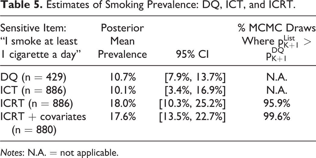
Notes: N.A. = not applicable.

ICRT Estimator

The analysis proceeded in two stages. In the first stage, we specified the sensitive proportion p_{K + 1} to be independent of respondent characteristics. Here, we use Equations 9 –15 and 17 –19, with an uninformative beta(1,1) prior for the sensitive proportion p_{K + 1}. In the second stage, we added information on respondent characteristics (described in the next subsection). We used 100,000 burn-in draws and the next 100,000 draws for inference.

The model fits the list data very well. Observed list counts are 56, 569, 240, and 21 (total n = 886) for list counts of, respectively, zero, one, two, and three, whereas average replicated frequencies (Equation 21) over the MCMC draws after burn-in are 58, 563, 245, and 20, respectively, for a 98% hit rate.⁴ In addition, when we use 750 of the 886 respondents to calibrate the model, and the remaining 136 respondents (16%) as a holdout sample, observed holdout frequencies are 6, 97, 31, and 2 for list counts of, respectively, zero, one, two, and three, whereas average replicated frequencies are 9, 85, 39, 3, respectively, for an 82% hit rate. Furthermore, we validated the ICRT differently, using a synthetic list that we compose in the DQ group.⁵ This validation shows that the ICRT can estimate back a known nonsensitive proportion for real data instead of simulation data. We discuss each component of the ICRT model for the treatment group next.

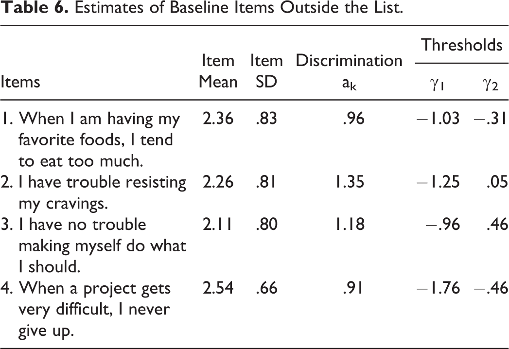
Baseline items outside the list

Item parameters of the baseline items outside the list are in Table 6. Although these items were measured on a five-point response scale, we noticed that the endpoints of the rating scale were rarely used. Therefore, we decided to collapse the endpoints of the response scale (merging “strongly disagree” and “disagree,” and “strongly agree” and “agree”) to create three-point response scales without loss of generality. Not doing so results in unstable first- and fourth-threshold estimates. Respondents mostly scored above the midpoint (two on the three-point response scale) for impulsiveness and self-discipline. The item parameter thresholds are well-separated. Most respondents have relatively moderate scores on the personality facets, which was already clear from the low frequencies of using the outer categories. This makes the items well-suited for the lists and ensures that the base rates are not too extreme. The baseline constructs are negatively correlated, with posterior mean correlation of −.292, which helps avoid ceiling effects (Glynn 2013).

Table 6.

Estimates of Baseline Items Outside the List.

Items	Item Mean	Item SD	Discrimination a_k	Thresholds
Items	Item Mean	Item SD	Discrimination a_k	γ₁	γ₂
1. When I am having my favorite foods, I tend to eat too much.	2.36	.83	.96	−1.03	−.31
2. I have trouble resisting my cravings.	2.26	.81	1.35	−1.25	.05
3. I have no trouble making myself do what I should.	2.11	.80	1.18	−.96	.46
4. When a project gets very difficult, I never give up.	2.54	.66	.91	−1.76	−.46

Procedural nonadherence

The posterior mean of the nonadherence probability is 19.0%, with 95% CI = [1.0%, 45.1%]. The posterior mean resembles the 22.9% biomarker-based noncompliance estimate reported in Dietz et al. (2011). Controlling for procedural nonadherence slightly improves model fit (LMD_withNA = −3,976.9 vs. LMD_withoutNA = −3,977.0).

Differential list functioning

Our ICRT model does not require a control group. However, in our research design, we do have a control group and can test the assumption of homogeneous list functioning that is required when using the standard ICT difference-in-means estimator. We use the machinery of measurement invariance testing (Holland and Wainer 1993; Steenkamp and Baumgartner 1998). If baseline items inside the list behave differently from baseline items in the DQ group, we have $a_{l i s t, k} \neq a_{D Q, k} and b_{l i s t, k} \neq b_{D Q, k} for k = 1, ..., K$ . We therefore compare item parameters in the list group and in the DQ group. Table 7 shows that the item parameters differ between the list and DQ groups.⁶ To formally test the differences between the item parameters, each MCMC draw assesses whether a specific item parameter is larger in the list group compared with the DQ group. Extreme values of below 5% or above 95% across MCMC draws after burn-in suggest significant differences in the values across the two groups. Indeed, there is strong evidence of differential list functioning: the difficulty parameter of the first baseline item is significantly larger in the list group than in the DQ group, and the converse holds for the second baseline item.

Table 7.

Item Parameters of Baseline Items Inside the List.

Item	ICRT		DQ		% of MCMC Draws Where a_{k, list} > a_{k, DQ}	% of MCMC Draws Where b_{k, list} > b_{k, DQ}
Item	a_{k, list}	b_{k, list}	a_{k, DQ}	b_{k, DQ}	% of MCMC Draws Where a_{k, list} > a_{k, DQ}	% of MCMC Draws Where b_{k, list} > b_{k, DQ}
Sometimes I do things on impulse that I later regret.	.52	1.03	.42	.32	74.5%	100%
I’m pretty good about pacing myself so as to get things done on time.	.61	−1.49	.72	−.91	28.9%	.00%

Notes: a = item discrimination; b = item difficulty.

These differences in item parameters have several consequences. As the simulations showed, prevalence estimates of the DQ group become much too low if the difficulty parameters of the baseline items are deflated. The differential list functioning results in a downward bias in the estimated prevalence of smoking during pregnancy in the DQ group.

To help interpret the item parameters, Figure 1 provides the item characteristic curves for the two baseline items inside the list for the list and DQ groups. Item characteristic curves show how the probability of an affirmative response varies as a function of the latent trait score. The latent trait score is on the x-axis and the probability of affirming the sensitive item (Pr[Z_{i, k} = 1]) is on the y-axis. For lower trait values, the probability of an affirmative response is close to zero. Item parameters are on the same scale as the latent trait.

Figure 1.

Item characteristic curves of inside baseline items in DQ group and list group.

Prevalence estimates

Table 5 shows that the ICRT prevalence estimate, which protects the respondent’s privacy and accounts for procedural nonadherence and differential list functioning, is indeed substantially higher than the prevalence estimate in the DQ group (18.0 vs. 10.7%, respectively). This percentage difference is in line with the reported percentage difference between DQ and biomarker estimates of smoking during pregnancy (Dietz et al. 2011; Lumley et al. 2009). Finally, the ICRT model with covariates, discussed next, estimates the prevalence to be 17.6%, which is also higher than in the DQ group.

We test the significance of the difference in prevalence estimates between DQ, standard ICT, and ICRT with a tail-area probability. We compute the fraction of the MCMC draws in which the prevalence estimate for the list group $p_{K + 1}^{L i s t}$ was larger than the estimate of the Bernoulli probability $p_{K + 1}^{D Q}$ in the DQ group. In the DQ group, we use the value of $p_{K + 1}^{D Q}$ in each draw from a beta posterior, with an uninformative beta(1,1) prior. The difference is deemed significant if the fraction exceeds 95%. Credible intervals of DQ, standard ICT, and ICRT overlap but are significantly different at 95% (Schenker and Gentleman 2001).

Although the 95% credible interval for the ICRT model without covariates is relatively wide, 95.9% of the $p_{K + 1}^{L i s t}$ draws are larger than the $p_{K + 1}^{D Q}$ draws. An important advantage of including covariates is that the 95% credible interval for p_{K + 1} narrows. Accounting for covariates greatly improves the precision of estimating smoking prevalence: a model with covariates outperforms a model without covariates (LMD_covariates = −3,907.2 vs. LMD_nocovariates = −3,976.9; both sample sizes = 880 to account for 6 respondents with missing data on the “weeks pregnant” variable).

The last row in Table 5 shows how well the predictors help to narrow the credible interval of the sensitive proportion p_{K + 1}. The improvement in precision is about 38% relative to the prevalence estimates of the ICRT without covariates, and as a result, 99.6% of the $p_{K + 1}^{L i s t}$ draws are larger than the $p_{K + 1}^{D Q}$ draws. This reveals not only that a substantial proportion of young women smokes during pregnancy but also that smoking prevalence is underreported when using direct questions and that accounting for covariates improves precision of the prevalence estimates. Importantly, the difference between the list and DQ groups is not driven by different sample characteristics because of successful random assignment (Table 4).

Drivers of Smoking Decision

In the second analysis stage, we estimated the ICRT model with Equation 16 instead of Equation 11 to relate the estimated smoking prevalence to covariates. Table 8 summarizes the results. Predictors are impulsiveness, self-discipline, and respondent’s age, number of children in the household, relationship status, number of weeks pregnant, education, current perceived socioeconomic status, and health locus of control. Uninformative normal priors were used for the regression coefficients.

Table 8.

Predicting Smoking Prevalence During Pregnancy.

	ICRT		DQ
	Mean	95% CI	Mean	95% CI
Intercept	−1.685	[−2.214, −1.263]	−2.442	[−4.188, −1.665]
Impulsiveness	−.451	[−.849, −.141]	−.927	[−2.313, −.264]
Self-discipline	−.405	[−1.021, −.009]	−.656	[−1.781, −.066]
Age	−.016	[−.055, .025]	−.055	[−.132, .003]
Number of children	.090	[−.141, .309]	.240	[−.034, .580]
Unmarried (1 = yes, 0 = no)	.643	[.241, 1.061]	.311	[−.180, .887]
Weeks pregnant	−.033	[−.054, −.013]	−.014	[−.041, .011]
Current socioeconomic status	−.379	[−.687, −.097]	−.051	[−.380, .288]
Education	−.416	[−.744, −.138]	−.453	[−1.027, −.069]
Health locus of control	−.490	[−.769, −.245]	−1.162	[−2.047, −.704]

Notes: 95% CI of boldfaced mean estimates does not include 0.

Except for the respondent’s age and the number of children in the household, all covariates are significantly related to smoking prevalence. In line with previous findings (Terracciano and Costa 2004), pregnant women with more self-discipline are less likely to smoke. Moreover, unmarried women are more likely to smoke. In fact, using the model estimates and holding all other covariates at their mean, smoking prevalence is estimated to be 4.6% among married women but 14.9% among unmarried women, which is more than three times higher. This difference is not due to differences in health locus of control, age, impulsiveness, and so on between unmarried and married pregnant women, because these variables were all statistically controlled for by the model, which makes the large difference even more telling.

The number of weeks that women were pregnant has a negative effect on smoking prevalence. Using the model estimates and holding all other drivers at their mean, smoking prevalence is estimated to be 18.1% after seven weeks of pregnancy but drops to 2.9% after 37 weeks. This reflects the increased urgency to stop smoking when pregnancy progresses and is in line with research documenting an increased effectiveness of smoking cessation interventions toward the end of pregnancy (Lumley et al. 2009). Women with higher levels of education and perceived socioeconomic status are less likely to smoke during pregnancy, which converges with other reports (Zimmer and Zimmer 1998). Furthermore, women with higher health locus of control scores are less likely to smoke during pregnancy.

Finally, we compare the covariate results of our model with the probit results in the DQ group. The latter results are obtained using the directly measured values for the three baseline items in the DQ group, instead of the augmented data {Z_i1, Z_i2}, U_i, as in the list group. There are several important differences between the regression results when stratifying by data collection method. In particular, marital status, number of weeks pregnant, and current socioeconomic status have no effect in the DQ group. Thus, above and beyond the significant difference in prevalence estimates between the ICRT and DQ, the ICRT method is also able to uncover more covariates that are related to smoking during pregnancy, which is notable in its own right.

General Discussion

We proposed the ICRT as a new truth-telling technique in consumer surveys about sensitive topics. The ICRT asks a single group of respondents to count how many items from a list of items they affirm, rather than whether they affirm each individual item from the list. The list contains several baseline items and the sensitive item of interest. This indirect way of asking questions protects respondents’ privacy and increases the likelihood of truthful responding as compared with direct questions about the sensitive behavior. The ICRT identifies the prevalence of the sensitive item by making use of the statistical association between baseline items inside the list and baseline items asked outside the list elsewhere in the questionnaire.

The ICRT introduces several innovations compared to earlier implementations of the ICT. First, the data collection design of the ICRT requires a single group of respondents only, rather than separate treatment and control groups. Thus, it makes more efficient use of the available survey resources, and it makes the assumption of group equivalence redundant. Second, the statistical model of the ICRT is the first to account for violations of procedural adherence and homogenous list functioning. By doing so, it provides more accurate prevalence estimates of the sensitive behavior than alternatives do. Third, the statistical model of ICRT facilitates multivariate analyses of potential drivers and correlates of the sensitive behavior at the individual level. This improves theory testing as well as policy decision making and evaluation. We provide specific recommendations for implementation of the ICRT subsequently.

The simulation results demonstrate the strengths of the ICRT model and have implications for existing ICT research, including controlled validation studies (Rosenfeld, Imai, and Shapiro 2016). The validity of ICT studies based on the standard ICT estimator that do not account for procedural nonadherence and differential list functioning is uncertain. The gain in validity of the estimates owing to the privacy protection provided by the ICT might be nullified by the loss in validity owing to violation of the ICT assumptions. To date, few ICT studies test for assumption violation (Blair and Imai 2012; Kuha and Jackson 2014).

We applied the ICRT to the domain of smoking behavior with a sample of 886 pregnant women, for which smoking is especially sensitive. We find evidence of substantial and significant underreporting when questions are asked directly, despite the standing practice in large scale research to rely on direct self-reports of smoking behavior during pregnancy (Bradford 2003; Lumley et al. 2009). Rather than merely establishing whether people smoke (or engage in other sensitive behaviors), ICRT also makes it easy to assess the drivers of smoking during pregnancy. This is relevant for theory testing and for the design and evaluation of smoking cessation interventions (e.g., http://www.acog.org). When pregnant women underreport their cigarette consumption, or cravings and feelings of being addicted, obstetricians, gynecologists and other professionals could deploy the wrong tools in cessation programs, with adverse health consequences (Lumley et al. 2009) and vast neonatal health care costs (Adams et al. 2002). Indeed, our findings indicate that several covariates (marital status, socioeconomic status, and number of weeks pregnant) that were insignificant in the direct questioning group were in fact significantly related to smoking during pregnancy when using the ICRT.

Implementation Recommendations

Analysts need to make various decisions when designing an item count study. Drawing on our theoretical analysis, simulation studies, and empirical applications, we formulate the following recommendations:

List size. A total list size of two to four items (K = 1, 2, or 3) is optimal. This range balances acceptable complexity of the respondent task with good statistical accuracy. Privacy protection is obviously greater for larger list sizes (five and up). Yet such larger list sizes complicate the respondent’s task and require undesirably high reliabilities (see the bullet point on reliability of scales) of the baseline trait measures of .90 to obtain precise prevalence estimates for the sensitive item, especially for low true-sensitive proportions.

Validated scales for baseline items. It is preferable to use K “inside” baseline items from K validated scales and administer remaining items from the scales “outside” the list. This will make the sensitive, target item in the list least salient, provides maximum privacy protection, and ensures trustworthiness of the procedure.

Negative correlation of scales. To reduce ceiling effects of the list sums that participants need to report and to reduce procedural nonadherence, we recommend selecting at least two negatively correlated validated baseline scales within the set of K validated scales.

Reliability of scales. The reliability of each of the K scales is preferably around .8, which is common for validated scales. Using validated scales with higher reliability (say .95) is undesirable. Such reliabilities usually require the use of conceptually and semantically similar items, which erodes privacy protection and trustworthiness of the list technique. Using validated scales with lower reliability (say .7 or less) reduces precision of the estimated prevalence of the target item.

Number of outside baseline items. It is recommendable to include for each validated scale k, at least two or three “outside” items elsewhere in the survey. Using more “outside” baseline items per validated scale k increases the burden to respondents and may not be needed in case reliable, short-form multi-item measures are available or easily developed.

Statistical model. Use of the ICRT statistical model for data analysis is preferable. Its better performance outweighs the added modeling effort. Follow-up analyses (details in Web Appendix 2) studied the performance of two simple benchmark models that, as the ICRT, also do not use information from a direct questioning group. The results indicate poor performance of these benchmark models and stress the importance of using the ICRT estimator. Whenever possible, we strongly recommend to collect relevant covariates (general and/or domain-specific covariates) that predict the the sensitive item. Using a probit equation for the sensitive item helps to narrow the credible interval of the sensitive proportion (which can otherwise be quite wide) and yields additional insights into the drivers of the sensitive behavior.

Opportunities and Future Developments

There are several opportunities for future methodological and substantive research. Methodologically, it would be interesting to compare the results of list-based questions with other privacy-protected questions, such as randomized response questions. Then strengths and weaknesses of various privacy protection techniques can be assessed. Initial attempts at such comparisons (Rosenfeld, Imai, and Shapiro 2016) could not yet model the response process to test crucial assumptions. That makes it difficult to assess the validity of such comparisons.

Substantively, it would be interesting to apply the ICRT across cultures to examine how people from different countries respond to the list-based questions, how the method’s accuracy varies across cultures compared with other types of privacy protection methods (e.g., randomized response), and how procedural nonadherence varies across countries. In a similar vein, the ICRT can be applied to obtain valid prevalence estimates of a host of other sensitive consumer behaviors wherein direct questions are likely to produce biased responses.

To return to the original challenge that motivated our research—as Jain (2017, p. 6) stressed, “The practice of computing smoking prevalence rates without adjusting for bias associated with self-reported smoking status is flawed.” The ICRT promises to be a valuable new addition to the toolbox of marketing and survey researchers who aim to know the prevalence of sensitive consumer behaviors, such as smoking status, by using self-reports, and the drivers of these behaviors. This might eventually help avert and curb the prevalence of such dark side and vice consumer behaviors.

Supplemental Material

Supplemental Material, jmr.17.0275_web_appendices - Assessing Sensitive Consumer Behavior Using the Item Count Response Technique

Supplemental Material, jmr.17.0275_web_appendices for Assessing Sensitive Consumer Behavior Using the Item Count Response Technique by Martijn G. de Jong and Rik Pieters in Journal of Marketing Research

Footnotes

Acknowledgments

The authors thank the JMR review team for their valuable suggestions and guidance throughout the review process. They have also benefited from comments by seminar participants at Vienna University.

Associate Editor

Peter Danaher served as associate editor for this article.

Declaration of Conflicting Interests

The author(s) declared no potential conflicts of interest with respect to the research, authorship, and/or publication of this article.

Funding

The author(s) disclosed receipt of the following financial support for the research, authorship, and/or publication of this article: Martijn G. de Jong thanks the Netherlands Organization for Scientific Research for research support.

Online supplement:

Notes

References

Adams

E. Kathleen

Miller

Vincent P.

Ernst

Carla

Nishimura

Brenda K.

Melvin

Cathy

Merrit

Robert

(2002), “Neonatal Health Care Costs Related to Smoking During Pregnancy,” Health Economics, 11 (3), 193–206.

Anderson

Drew A.

Simmons

Angela M.

Milnes

Suzanne M.

Earleywine

Mitchell

(2007), “Effect of Response Format on Endorsement of Eating Disordered Attitudes and Behaviors,” International Journal of Eating Disorders, 40 (1), 90–93.

Andrews

J. Craig

Netemeyer

Richard G.

Burton

Scot

Moberg

D. Paul

Christiansen

Ann

(2004), “Understanding Adolescent Intentions to Smoke: An Examination of Relationships Among Social Influence, Prior Trial Behavior, and Antitobacco Campaign Advertising,” Journal of Marketing, 68 (3), 110–23.

Bearden

William O.

Netemeyer

Richard G.

Haws

Kelly L.

(2011), Handbook of Marketing Scales. Multi-Item Measures for Marketing and Consumer Behavior Research, 3rd ed. Thousand Oaks, CA: SAGE Publications.

Blair

Graeme

Imai

Kusuke

(2012), “Statistical Analysis of List Experiments,” Political Analysis, 20 (1), 47–77.

Bradford

W. David

(2003), “Pregnancy and the Demand for Cigarettes,” American Economic Review, 93 (5), 1752–63.

Bradlow

Eric T.

Wainer

Howard

Wang

Xiaohui

(1999), “A Bayesian Random Effects Model for Testlets,” Psychometrika, 64 (2), 153–68.

Coffman

Katherine B.

Coffman

Lucas C.

Ericson

Keith M. Marzilli

(2017), “The Size of the LGBT Population and the Magnitude of Anti-Gay Sentiment Are Substantially Underestimated,” Management Science, 63 (10), 3168–86.

Corstange

Daniel

(2009), “Sensitive Questions, Truthful Answers? Modeling the List Experiment with LISTIT,” Political Analysis, 17 (1), 45–63.

10.

Costa

Paul T.

McCrae

Robert R.

(2008), “The Revised NEO Personality Inventory (NEO-PI-R),” in The SAGE Handbook of Personality Theory and Assessment: Personality Measurement and Testing, Vol. 2, Boyle

Gregory J.

Matthews

Gerald

Saklofske

Donald H.

, eds. London: SAGE Publications.

11.

Cui

Yang

Shoostari

Shahin

Forget

Evelyn L.

Clara

Ian

Cheung

Kwong F.

(2014), “Smoking During Pregnancy: Findings from the 2009-2010 Canadian Community Health Survey,” PLOS ONE, 9 (1), 1–5.

12.

De Jong

Martijn G.

Pieters

Rik

Fox

Jean-Paul

(2010), “Reducing Social Desirability Bias Through Item Randomized-Response: An Application to Measure Under-Reported Desires,” Journal of Marketing Research, 47 (1), 14–27.

13.

Dietz

Patricia M.

Homa

David

England

Lucinda J.

Burley

Kim

Tong

Van T.

Dube

Shanta R.

. (2011), “Estimates of Nondisclosure of Cigarette Smoking Among Pregnant and Nonpregenant Women of Reproductive Age in the United States,” American Journal of Epidemiology, 173 (3), 355–59.

14.

Ding

Min

Grewal

Rajdeep

Liechty

John

(2005), “Incentive-Aligned Conjoint Analysis,” Journal of Marketing Research, 42 (1), 67–82.

15.

Fox

Jean-Paul.

Avetisyan

van der Palen

Job

(2013), “Mixture Randomized Item-Response Modeling: A Smoking Behavior Validation Study,” Statistics in Medicine, 32 (27), 4821–37.

16.

Fox

Jean-Paul

Glas

Cees A.W.

(2001), “Bayesian Estimation of a Multilevel IRT Model Using Gibbs Sampling,” Psychometrika, 66 (2), 271–88.

17.

Geisser

Seymour

Eddy

William

(1979), “A Predictive Approach to Model Selection,” Journal of the American Statistical Association, 74 (365), 153–60.

18.

Glynn

Adam

(2013), “What Can We Learn With Statistical Truth Serum? Design and Analysis of the List Experiment,” Public Opinion Quarterly, 77 (S1), 159–72.

19.

Griskevicius

Vladas

Tybur

Joshua M.

Delton

Andrew W.

Robertson

Theresa E.

(2011), “The Influence of Mortality and Socioeconomic Status on Risk and Delayed Rewards: A Life History Theory Approach,” Journal of Personality and Social Psychology, 100 (6), 1015–26.

20.

Hackshaw

Allan

Rodeck

Charles

Boniface

Sadie

(2011), “Maternal Smoking in Pregnancy and Birth Defects: A Systematic Review Based on 173,687 Malformed Cases and 11.7 Million Controls,” Human Reproduction Update, 17 (5), 589–604.

21.

Holland

Paul W.

Wainer

Harold

(1993), Differential Item Functioning. Hillsdale, NJ: Lawrence Erlbaum Associates.

22.

Hyman

Steven E.

(2001), Personality and Personality Disorder (The Science of Mental Health, Vol. 7), 1st ed. New York: Routledge.

23.

Imai

Kosuke

(2011), “Multivariate Regression Analysis for the Item Count Technique,” Journal of the American Statistical Association, 106 (494), 407–16.

24.

Imai

Kosuke

Park

Bethany

Greene

Kenneth F.

(2015), “Using the Predicted Responses from List Experiments as Explanatory Variables in Regression Models,” Political Analysis, 23 (2), 180–96.

25.

Jain

Ram B.

(2017), “Analysis of Self-Reported Versus Biomarker Based Smoking Prevalence: Methodology to Compute Corrected Smoking Prevalence Rates,” Biomarkers, 22 (5), 1–17, doi:10.1080/1354750X.2016.1278264

26.

John

Leslie K.

Acquisti

Allessandro

Loewenstein

George

(2011), “Strangers on a Plane: Context-Dependent Willingness to Divulge Sensitive Information.” Journal of Consumer Research, 37 (5), 858–73.

27.

Kuha

Jouni

Jackson

Jonathan

(2014), “The Item Count Method For Sensitive Survey Questions: Modelling Criminal Behaviour,” Journal of the Royal Statistical Society: Series C (Applied Statistics), 63 (2), 321–41.

28.

Kuklinski

James H.

Cobb

Michael D.

Gilens

Martin

(1997), “Racial Attitudes and the New South,” Journal of Politics, 59 (2), 323–49.

29.

Lamb

Charles W.

Stem

Donald E.

(1978), “An Empirical Validation of the Randomized Response Technique,” Journal of Marketing Research, 15 (4), 616–21.

30.

Lumley

Judith

Chamberlain

Catherine

Dowswell

Therese

Oliver

Sandy

Oakley

Laura

Watson

Lyndsey

(2009), “Interventions for Promoting Smoking Cessation During Pregnancy,” Cochrane Database Systematic Reviews, 3, 1–124.

31.

Marshall

Margarita B.

Rolland

Jean-Pierre

de Fruyt

Filip

Michael Bagby

(2005), “Socially Desirable Responding and the Factorial Stability of the NEO PI-R,” Psychological Assessment, 17 (3), 379–84.

32.

Moorman

Christine

Matulich

Erika

(1993), “A Model of Consumers’ Preventive Health Behaviors: The Role of Health Motivation and Health Ability,” Journal of Consumer Research, 20 (3), 208–28.

33.

Nepusz

Tamas

Petróczi

Andrea

Naughton

Declan P.

Epton

Tracy

Norman

Paul

(2014), “Estimating the Prevalence of Socially Sensitive Behaviors: Attributing Guilty and Innocent Noncompliance with the Single Sample Count Method,” Psychological Methods, 19 (3), 334–55.

34.

Petróczi

Andrea

Nepusz

Tamás

Cross

Paul

Taft

Helen

Sha

Syeda

Deshmukh

Nawed

. (2011), “New Non-Randomised Model to Assess the Prevalence of Discriminating Behaviour: A Pilot Study on Mephedrone,” Substance Abuse Treatment, Prevention, and Policy, 6, 1–18.

35.

Rosenfeld

Bryn

Imai

Kosuke

Shapiro

Jacob N.

(2016), “An Empirical Validation Study of Popular Survey Methodologies for Sensitive Questions,” American Journal of Political Science, 60 (3), 783–802.

36.

Rossi

Peter H.

Allenby

Greg

McCulloch

Rob

(2005), Bayesian Statistics and Marketing. West Sussex, UK: John Wiley & Sons.

37.

Samejima

Fumiko

(1969), Estimation of Latent Ability Using a Response Pattern of Graded Scores (Psychometric Monograph No. 17). Richmond, VA: Psychometric Society. Retrieved from http://www.psychometrika.org/journal/Online/MN17.pdf.

38.

Schenker

Nathaniel

Gentleman

Jane F.

(2001), “On Judging the Significance of Differences by Examining the Overlap Between Confidence Intervals,” American Statistician, 55 (3), 182–86.

39.

Spiegelhalter

David J.

Thomas

Andrew

Best

Nicky G.

Gilks

Wally

(1996), BUGS 0.5: Bayesian Inference Using Gibbs Sampling–Manual (Version ii). Cambridge, UK: Medical Research Council Biostatistics Unit.

40.

Steenkamp

Jan-Benedict E.M.

Baumgartner

Hans

(1998), “Assessing Measurement Invariance in Cross-National Consumer Research,” Journal of Consumer Research, 25 (1), 78–90.

41.

Tanner

Martin A.

Wong

Wing Hung

(1987), “The Calculation of Posterior Distributions by Data Augmentation,” Journal of the American Statistical Association, 82 (39), 528–50.

42.

Terracciano

Antonio

Costa

Paul T.

(2004), “Smoking and the Five-Factor Model of Personality,” Addiction, 99 (4), 472–81.

43.

Tian

Guo-Liang

Tang

Man-Lai

Qin

Liu

Yin

(2014), “Poisson and Negative Binomial Item Count Techniques for Surveys with Sensitive Question,” Statistical Methods in Medical Research, 26 (2), 1–17.

44.

Tourangeau

Roger

Yan

Ting

(2007), “Sensitive Questions in Surveys,” Psychological Bulletin, 133 (5), 859–83.

45.

Wang

Yanwen

Lewis

Michael

Singh

Vishal

(2016), “The Unintended Consequences of Countermarketing Strategies: How Particular Antismoking Measures May Shift Consumers to More Dangerous Cigarettes,” Marketing Science, 35 (1), 55–72.

46.

Weaver

Ray

Prelec

Drazen

(2013), “Creating Truth-Telling Incentives with the Bayesian Truth Serum,” Journal of Marketing Research, 50 (3), 289–302.

47.

Wolter

Felix

Laier

Bastian

(2014), “The Effectiveness of the Item Count Technique in Eliciting Valid Answers to Sensitive Questions. An Evaluation in the Context of Self-Reported Delinquency,” Survey Research Methods, 8 (34), 153–68.

48.

Wolter

Felix

Preisendorfer

Peter

(2013), “Asking Sensitive Questions: An Evaluation of the Randomized Response Technique Versus Direct Questioning Using Individual Validation Data,” Sociological Methods & Research, 42 (3), 321–53.

49.

Zimmer

Martha Hill

Zimmer

Michael

(1998), “Socioeconomic Determinants of Smoking Behavior During Pregnancy,” Social Science Journal, 35 (1), 133–42.

Supplementary Material

Please find the following supplemental material available below.

For Open Access articles published under a Creative Commons License, all supplemental material carries the same license as the article it is associated with.

For non-Open Access articles published, all supplemental material carries a non-exclusive license, and permission requests for re-use of supplemental material or any part of supplemental material shall be sent directly to the copyright owner as specified in the copyright notice associated with the article.

0.00 MB

0.39 MB