Sage Journals: Discover world-class research

Abstract

Laser-assisted tape winding is an automated process to produce tubular or tube-like continuous fiber-reinforced polymer composites by winding a tape around a mandrel or liner. Placing additional layers on a previously heated substrate and variation in material and process parameters causes a variation in the bonding temperature of fiber-reinforced thermoplastic tapes which need to be understood and described well in order to have a reliable manufacturing process. In order to quantify the variation in this critical bonding temperature, a comprehensive temperature analysis of an adjacent hoop winding process of type-IV pressure vessels is performed. A total of five tanks are manufactured in which three glass/HDPE tapes are placed on an HDPE liner. The tape and substrate temperatures, roller force and tape feeding velocity are measured. The coefficient of variation for each round is characterized for the first time. According to the statistical analysis, the coefficient of variation in substrate temperature is found to be approximately 4.8–8.8% which is larger than the coefficient of variation of the tape temperature which is 2.1–7.8%. The coefficient of variations of the substrate temperatures in the third round decrease as compared with the coefficient of variations in the second round mainly due to the change in gap/overlap behavior of the deposited tapes. Fourier and thermographic analysis evince that the geometrical disturbances such as unroundness and eccentricity have a direct effect on the temperature variation. In addition to the temperature feedback control, a real-time object detection technique with deep learning algorithms can be used to mitigate the unwanted temperature variation and to have a more reliable thermal history.

Keywords

Laser-assisted tape winding thermoplastic composites experimental analysis coefficient of variation

Introduction

New fuel regulations and emission restrictions in the transport sector increase the appeal of lightweight composite components. Especially, thermoplastic composites experience a rise in applications due to their unique characteristics, including repeated shapeability and recyclability.¹ Manufacturing of sustainable products with respect to challenging environmental influences, quick adaptability, failure-free quality and safe operation over the complete life cycle is mandatory. The lightweight components like composite pressure vessels for the storage of hydrogen² or compressed natural gas (CNG) are gaining appeal within the automotive and transport industries.¹ Pressure vessels with a full composite design (type IV – an all-composite construction featuring a polymer liner with carbon or glass fiber reinforcement) exhibit relatively high specific strength and rigidity as well as corrosion resistance.^3,4 The combination of a thermoplastic liner with composite reinforcements to substitute conventional metal designs enables relatively high internal gas pressures, which together with the reduced pressure vessel weight adds to the range (longer distance) of fuel-cell based or CNG applications.⁵ For this type of lightweight pressure vessels, HDPE (high-density polyethylene) is often selected as a durable solid material which can dampen and absorb shock waves minimizing surges as well as the abrasion resistance. This polymer material is well-suited for industrial, automotive and sporting goods applications where cost and processability are critical.^6–8 Regarding the reinforcement tapes, glass fiber (GF)-reinforced tape is preferred for low-pressure applications rather than carbon fiber (CF) tapes due to pricing, higher durability and more mechanical flexibility (carbon fibers are more rigid).⁹ Thus, the manufacturing of glass fiber-reinforced type-IV pressure vessels is highly favored in high-volume applications, where low unit cost is a priority.

One of the advanced techniques to make tubular long or continuous fiber-reinforced thermoplastic (CFRTs) components like pressure vessels is laser-assisted tape winding (LATW).¹⁰ LATW has been a source of great interest to attain higher composite part accuracy and quality but with reduced cycle times. The LATW process relies on heating through diode lasers similar to laser-assisted tape placement (LATP). These diode lasers are preferred over alternative heating sources, e.g. hot gas or infrared emitters, due to their high energy concentration, short response times and excellent controllability for ensuring an ideal heat input adapted to the current process velocity.^10,11 Another advantage of the LATW process is avoiding additional curing steps which makes it more time-efficient in comparison with competing thermoset composite manufacturing technologies.¹² This is achieved via in situ consolidation of the thermoplastic unidirectional fiber-reinforced tape and the substrate, which are simultaneously heated by a focused laser spot in the process zone while the pressure is applied to the substrate surface and the tape simultaneously.

In Figure 1, a typical hoop-winding case is shown where the tape and substrate are heated by the laser source on a cylindrical liner. The winding path in a continuous LATW process is designed such that it includes transitions between different angles in subsequent layers. The process can be used for the manufacturing of either concluded products like pressure vessels or continuous ones like pipes for oil and gas recovery in offshore deep-sea applications depending on the actuating system technology guiding the tape winding head.¹³

Figure 1.

Description of the LATW elements including laser optics, substrate, tape, roller, and liner. The hoop-winding process where thermoplastic tape and substrate are preheated by the laser source and the tape is pressed on the substrate at the nip-point location through a consolidation roller is shown as: (a) Principle and (b) System technology (detailed view on the experimental set-up employed at Fraunhofer IPT, Aachen, Germany).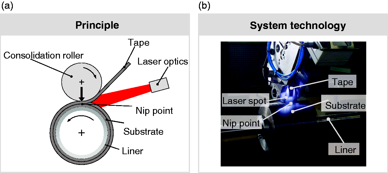

Optimum process conditions are needed to ensure good consolidation and adhesion between subsequent layers.¹⁴ The bonding temperature at the location where incoming tape and the substrate come in contact, the so-called nip-point, is widely regarded as the most important parameter among the process variables governing the consolidation quality.¹⁵ Kok¹⁶ clearly stated that unwanted overheating causes negative effects on intralaminar void content, intralaminar bond strength and residual stresses. Several efforts have therefore been made towards analyzing the temperature distributions on the substrate and incoming tape to define the nip-point temperature, e.g. Del Castillo et al.¹⁷ used fiber-Bragg grating (FBG) sensors and a thermocouple, Stokes-Griffin et al. and Schäkel et al.^18–20 used thermocouples and Perez et al.²¹ used an infrared thermographic camera. In Weiler et al.²², carbon fiber-reinforced PA12 composites were employed for the LATP process on flat surfaces. Other thermoplastic materials like PEEK CF, PPS CF and PA6 CF were also utilized for placement on flat surfaces as discussed in literature^23–25respectively. For a continuous ring winding (circular shape) via the LATW process, Reichardt²⁶ performed an experimental and a numerical study on PEEK CF.

In order to have a reliable and consistent product performance, the bonding temperature at the nip-point should remain at a constant, optimized value for each deposited layers. However, it is very difficult to achieve a constant nip-point temperature due to the following phenomena that inherently take place in LATP/LATW processes:

variation in material properties²¹;

variation in fiber volume fraction and distribution in the tape and substrate²¹;

variation in porosity, roughness and thickness in the incoming tape²¹;

variation in the geometrical position of the deposited tapes which can result in gaps and overlaps in the substrate²⁷;

variation in the roller force due to the variation in the local stiffness of the mold/mandrel or deformation of the roller.

These variations directly influence the absorption and reflection behavior of the tape and substrate which are fiber orientation and incident angle dependent.²⁸ In addition, the previously deposited layer’s temperature in a continuous LATW process has an influence on the nip-point temperature. A variation in the roller force results in a variation in the local deformation in roller and/or substrate which affects the location of the nip-point and local reflections on the tape and substrate. The process parameters have therefore to be controlled in order to compensate for such variations in temperature during the process. In Perez et al.,²¹ the effects of variation in material properties, thickness and fiber volume fraction on the substrate temperature were studied statistically in an LATW of AS4/PEEK composites. A coefficient of variation of approximately 2.5–5% was estimated for the temperature variation in the range of approximately 9–20℃. It was concluded that the uncertainties in the material properties and process dynamics can result in a significant variation in the thermal response with considerable impact on the industrial applications. However, apart from this study, in literature, there has been no study on the variation in tape and substrate temperature during continuous LATW of thermoplastic composites by taking the geometrical disturbances into account. The determination of the coefficient of variation (COV) in temperature evolution is utmost important for reliable continuous LATW processes and process optimization.

Understanding the process temperature development and describing the variations in material temperature and process parameters are key in order to develop proper computational models and in-line process control strategies for LATW of thermoplastic composites.^29,30 Therefore, the main objective of this paper is to analyze the temperature evolution quantitatively and statistically by a closer look at the variations in the process parameters and setup. The analysis of the temperature development during an adjacent continuous hoop winding process of a type-IV pressure vessel is presented in this paper. A total of five vessels were manufactured in which the temperature distribution in the tape and substrate was measured using an infrared thermal camera. The measurements were performed only for the LATW of the first three layers which were deposited on a thermoplastic liner. A statistical characterization of the measured tape and substrate temperature was made for each layer together with the variation in roller force and tape feeding velocity for the first time in literature. The influence of the geometrical disturbances, such as dimensional irregularities in the liner, on the temperature was determined by using thermographic images and employing a Fourier analysis of temperature, roller force and tape feeding velocity.

Experimental work

The composite pressure vessels were manufactured with the in-house developed PrePro3D system at Fraunhofer IPT. The type-IV pressure vessels consist of a polymer liner and additional adjacent hoop and helical fiber-reinforced tape layers. This section describes the materials and the method for the manufacturing of thermoplastic composite pressure vessels.

Materials and setup

The pressure vessel was composed of a blow-molded HDPE polymer liner and a number of layers of a unidirectional (UD) tape of glass fibers embedded in an HDPE matrix. The utilized UD-tape was Celstran CFR-TP HDPE GF70-01, which was a 70% E-glass by weight with a fiber volume fraction of 47%.³¹ The tape thickness was 0.25 mm and the tape was slit to a width of 25 mm for adjacent hoop winding on the cylindrical part of the liners. The melting temperature of the HDPE ranges between 108 and 134℃.³² The dimensional specifications of the 40-liter tank liners are shown in Figure 2. The blow-molded polymer liners provided by HBN-Teknik A/S exhibited a nominal thickness of 5 mm and were equipped with boss pieces out of polymer and metal at the dome parts. The laser absorption of the tank liner is sensitive to the composition of the HDPE, the tank liner thickness, possible heat treatments, the amount and type of pigments added and the surface finishing.^15,32,33 The blow molded HDPE liner employed in this research featured a relatively small edge due to the mold parting line as indicated in Figure 2. The rough dimensions of the mold parting line on the cylindrical part were 0.5 mm as width and 0.1 mm as height which may affect the temperature evolution locally. The connection between the tank liner and the rotating pipe was made by six screw elements. The rotating pipe was supported by two bearings with 58 mm distance to the tank liner. There were also two bearings supporting the tank liner in direct contact on the other side of the tank liner (end of cylindrical part of the tank liner).

Figure 2.

Schematic of 40-l tank liner dimension (640.4 mm as length and 272 mm as diameter), the blow-molded edge along tank length and fixation of tank liner with the pipe by screw elements and bearings are shown. The rough dimensions of the blow-molded edge on the cylindrical part are 0.5 mm (width) and 0.1 mm (height).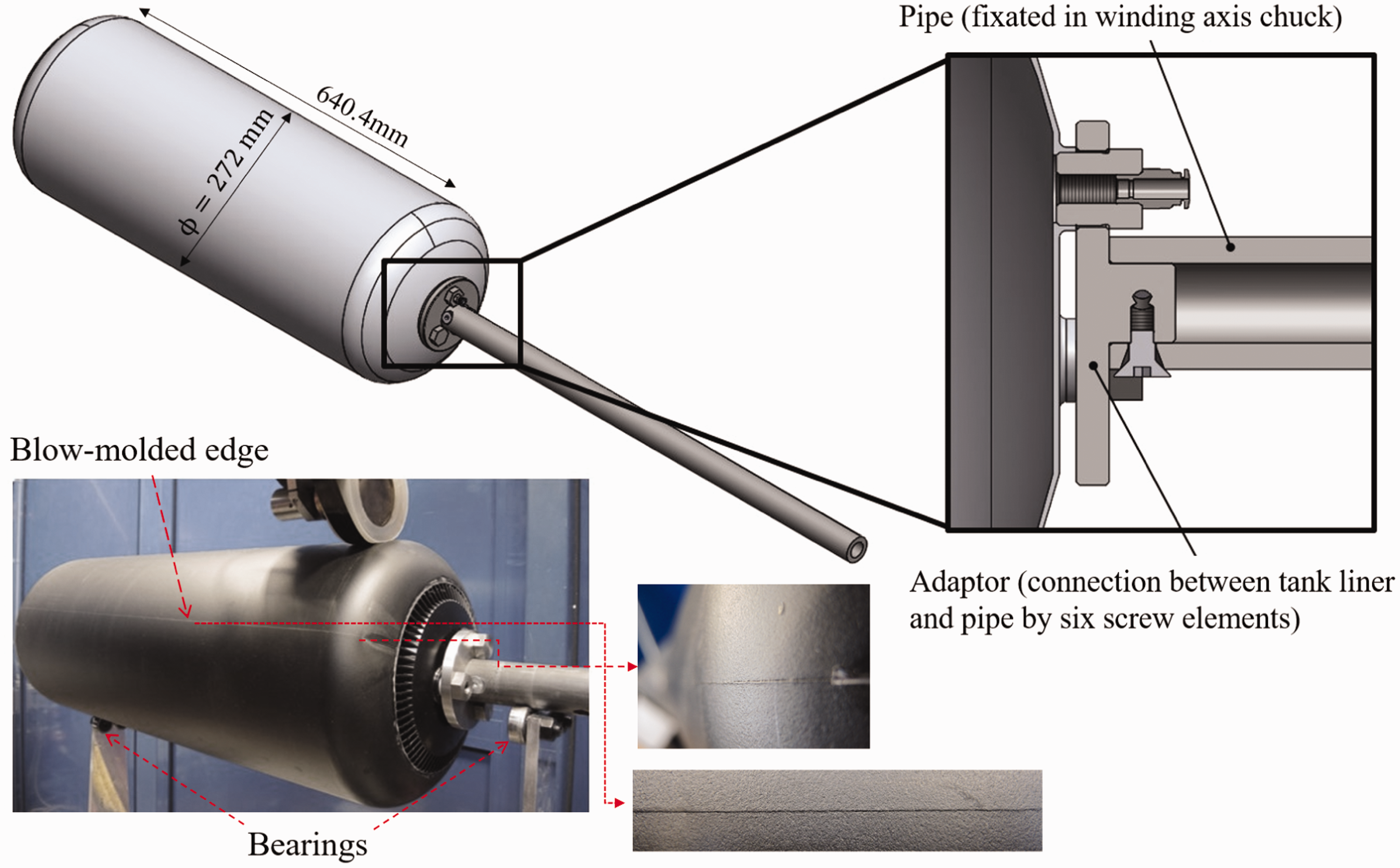

The processing of the pressure vessel liners was executed with time independent constant input parameters based on processing knowledge of Fraunhofer IPT and initial parameter trials as no data were available in literature for processing of glass/HDPE thermoplastic tape through LATW. Further details regarding the process parameter selection are not mentioned here, since the focus of this paper is solely on the characterization of the variation in temperature during continuous LATW of glass HDPE tanks.

On the basis of the cumulated results of all trials, the deposition velocity of the reinforcing tape was set to a nominal value of 140 mm/s, the laser power was kept constant at 900 W and the compression force exerted by the consolidation roller was set to a nominal value of 105 N as the threshold for ensuring sufficient intimate contact. The force was exerted by the flexible roller developed by Fraunhofer IPT³⁴ and can be modeled as a spring-damper system.

An LDF 3000-40 VGP diode laser with wavelength of 935–1030 nm ± 10 nm and the total laser power 3300 W cw by Laserline GmbH was employed as a heating source.³⁵ The laser power remained constant during the process. A uniformly distributed rectangular laser spot size of 14 × 28 mm at the aperture was realized by the laser optics which is represented in Figure 3. This rectangular spot became larger due to the laser divergence at the nip-point, similar to the configuration represented in Stokes-Griffin and Compston.³⁶ The size of the irradiated area at the nip-point which was approximately 400 mm away from the laser optics had a length of 67 mm and a width of 32 mm on a plane parallel to the laser aperture.³⁷ The spot size was determined as larger than the tape width to ensure covering the whole material surface by the laser irradiation.

Figure 3.

Schematic view of the laser source characteristics including laser intensity distribution and profile. The laser optics was attached to the winding head which was ∼400 mm away from the nip-point. The laser divergence caused a larger laser spot as 32 × 67 mm at the nip-point.^35,37 The pink color in the snapshot image represents the laser which is irradiated on the tape, roller and liner at the beginning of the process (for interpretation of the references to color in this figure legend, the reader is referred to the web version of this article).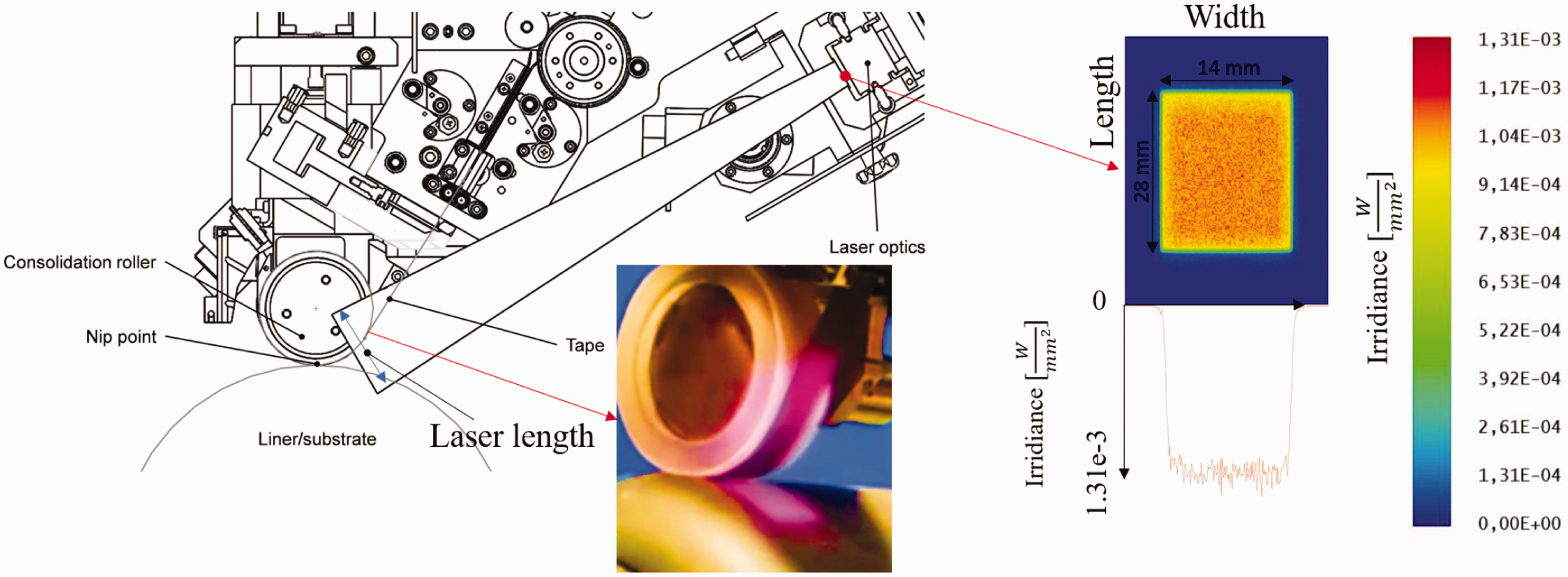

The dimensional configuration of the assembled laser optics is seen in Figure 4 (in this picture, φ₁ and φ₂ are 28° and 32°, S₁ and S₂ are 370 mm and 210 mm, respectively).

Figure 4.

Schematic of LATW setup configuration of pressure vessel manufacturing. Moving direction of liner and consolidation roller, tape feed direction, laser optics, thermal imaging camera (TIC), substrate and spring-damper system are shown in this picture. φ₁ and φ₂ are 28° and 32°, S₁ and S₂ are 370 mm and 210 mm, respectively.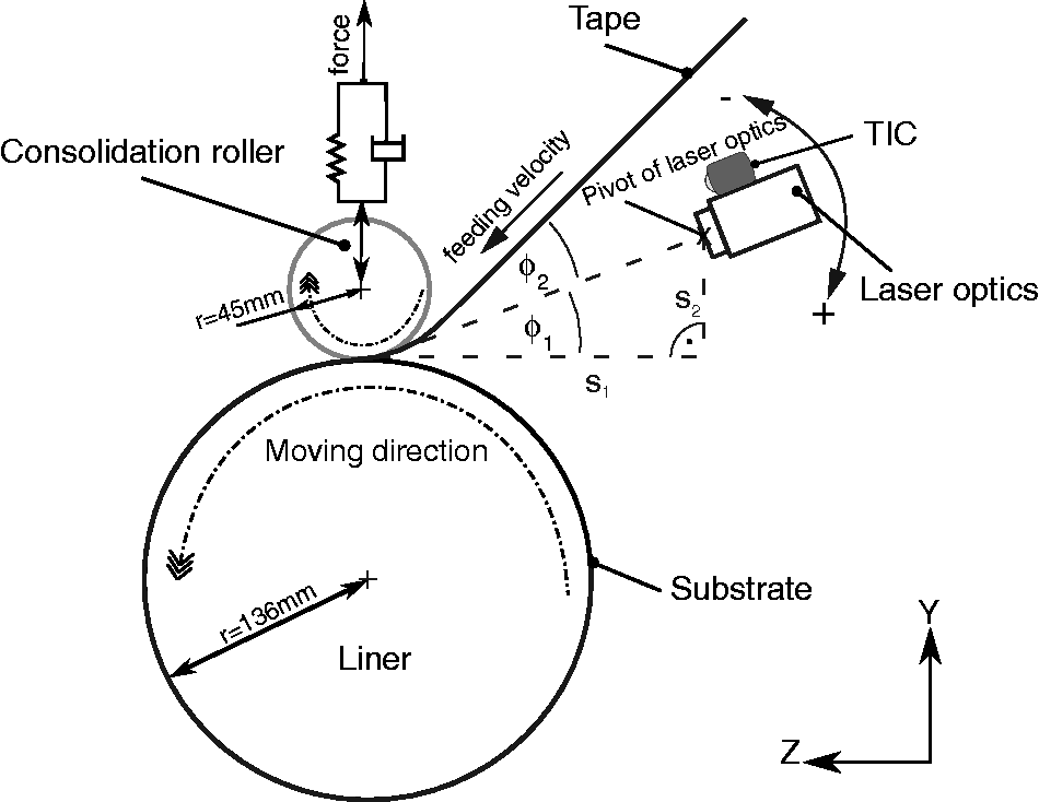

The measurement of the tape and substrate temperature was carried out with an infrared thermographic camera from DIAS Infrared (type: Pyroview 380Lc) located just above the laser optics enabling image acquisition at frame rates of 50 Hz. The technical specification of the infrared thermographic camera consists of: aperture angle as 22° × 16°, spectral range as 8–14 µm, measurement temperature range as 0–500℃, resolution as 384 × 288 pixel. The sensor was based on an uncooled microbolometer array with a measurement uncertainty of approximately 2 K when the object temperature is below 100℃ and otherwise 2% of the measurement value in ℃. The more details of thermographic temperature acquisition, the control interface, data transmission and imaging can be found in Brecher et al.³⁸

Characteristic average values for the tape and substrate temperature were extracted from the acquired images from areas of 5 × 5 mm² located at a distance of 10 mm above and below the nip-point, respectively. The measurement zones were chosen based on experience and best practice from Fraunhofer IPT. The determined measurement areas are shown in the thermographic camera image in Figure 5.

Figure 5.

(a) Thermographic image from DIAS Infrared (type: Pyroview 380Lc) for extracting tape and substrate temperatures from indicated areas (boxes) during the LATW process. In this image, isothermal regions are shown with their boundaries on the tape and substrate. (b) The distance “A-B” is realized between the tape edge (to be placed) and the edge of substrate (already wound) at the nip-point in the first round (winding on polymer liner surface). This distance indicates creation of gap or overlap in the first round (for interpretation of the references to color in this figure legend, the reader is referred to the web version of this article).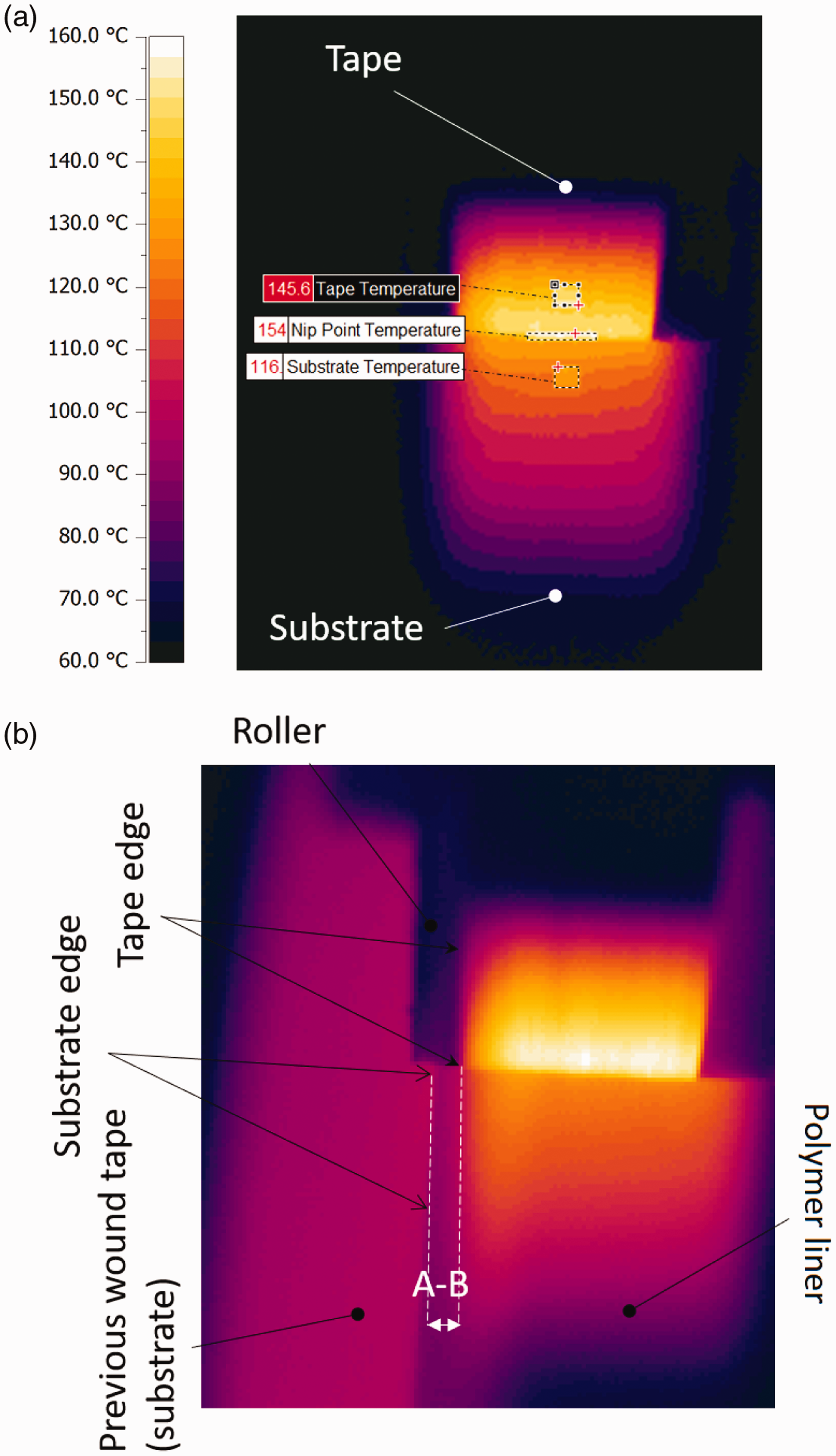

A thermographic image during the lay-up process in the first round is also illustrated in Figure 5(b) which indicates the formation of gap/overlap due to geometrical disturbances such as unroundness and eccentricity. Distance “A-B” between the tape edge (to be placed) and the edge of substrate (already wound tape) shown in Figure 5(b) indicates the gap formation during the first round. A positive value of this parameter shows the gap between these two edges, a negative distance shows the overlap on two edges and zero value of “A-B” distance indicates a perfect lay-up regarding geometry.³⁷

The average temperature values of the measurement areas were extracted and employed for the analysis in this paper.

The emission coefficient of the UD glass/HDPE thermoplastic prepreg tape for extracting temperature is temperature and angle dependent (angle of thermal camera toward the material). The value of emission coefficient employed for the temperature calculation by the camera software (PYROSOFT version 3.17.0.3 from DIAS Infrared GmbH) was set to 0.9 based on emission coefficient measurements performed with the glass/HDPE fiber-reinforced tape (see possible sources of non-contact measurement error in Appendix 1).

The value was set to 0.6 for the pure HDPE liner surface at the first round when the tape was deposited directly on the liner (the value was derived based on the experimental analysis in Abdel-Ghany et al.³⁹). Additional sensors were embedded in the tape winding head to transmit actual values of the tape tension, compression force and tape feed velocity which is seen in Figure 6. The tape and substrate temperature as well as other measured parameters were recorded throughout the LATW process for tank reinforcement by an in-house developed Beckhoff-based programmable logic controller (PLC). It can monitor the process stability and give the operator the possibility of in-process adjustments, if the values lie outside of predefined and knowledge-based process boundaries. This model also regulates the compression force against possible misalignments in the system, i.e. gaps and overlaps in the deposited tape²⁷ via a closed-loop control in order to keep enough contact between the consolidation roller and the tank liner.⁴⁰

Figure 6.

Sensors locations for measuring tape tension, tape feeding velocity and roller force. The locations of the tape and tape feeding spool are also shown.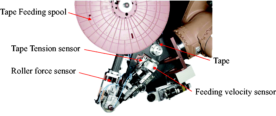

Process kinematics

The HDPE tank liners were reinforced with seven layers (executed through seven rounds) of tape on top of each other according to the requirements set by desired burst pressure and determined layup. The total reinforcement thickness is equal to 1.75 mm. First, three rounds of adjacent hoop layers were applied continuously on the cylindrical part, followed by four rounds of helical layers covering the entire liner including cylindrical and dome parts. The focus of this paper is on the adjacent hoop winding of the tapes on the tank liner. Successful implementation of these layers is important to the quality of the end product and key phenomena observed and understood with this process can also be applied to the case of the more complicated helical winding process that will be studied at a later stage. The kinematic of the adjacent hoop winding process is outlined as a lateral movement of the tape winding head from the beginning to the end of the cylindrical part, while the tank liner is rotating at a constant angular speed. During this movement, a possible eccentricity might occur due to the fixation setup and deformation of the tank liner (see “Materials and setup” section). The eccentricity generates a distance between the tank liner axis and the rotation axis which may result in a variation in the tape feeding velocity and roller force. The system technology accounts for this possible eccentricity by a spring suspension of the compression roller, which is able to maintain a constant pressure value in the nip-point. However, this adjusting movement leads to deviations in the nip-point location observed by the stationary thermographic infrared camera and irradiated by the stationary laser optics.

The winding angle was determined as ±88.2° which allows the continuous adjacent winding of the tapes (25 mm width) on a liner with 272 mm diameter. The end position of one round constitutes the start position for the next round as the adjacent hoop winding was executed continuously. After the first round, the moving direction is reversed and the head is laterally moving back to the beginning of the cylindrical part of the liner (round 2).

This transition from one round to the next round also includes changing winding direction which is amounted as 3.6° (changing winding angle from +88.2° to −88.2° or vice versa).

This procedure continues for three rounds as shown schematically in Figure 7. In each round, the liner rotates 22 times resulting in a placement of 22 adjacent annular cycles of the tape. Each round of adjacent hoop winding takes roughly 134 seconds based on the average tape feed velocity, liner diameter, winding angle, and length of the cylindrical part of the liner (∼640.4 mm). Thus, winding three rounds on a tank takes roughly 6 min and 43 s (∼403 s). The described procedure in this section for manufacturing type-IV pressure vessel was executed for five tanks in a similar way in order to have reliable and repeatable results.

Figure 7.

Schematic view of continuous winding kinematics for three rounds of adjacent hoop winding on the cylindrical part of the HDPE tank liner. The winding angle was ±88.2°.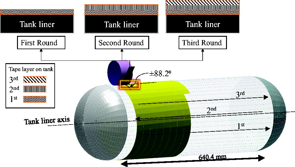

Results and discussion

An interim and a final result of pressure vessel manufacturing through the LATW process are shown in Figure 8. One of the products is visible after three rounds of adjacent hoop winding and a final product followed by four rounds of helical winding covering the entire tank liner. This section focuses on the explanation of the observed phenomena during the first three rounds of adjacent hoop winding (see Figure 8(a)). It also provides an assessment of process stability and repeatability.

Figure 8.

(a) Tank liner at the end of three rounds of adjacent hoop winding and (b) the final product of pressure vessel including three rounds of adjacent hoop layers followed by four rounds of helical layers covering the entire body (see section “Experimental work” for description).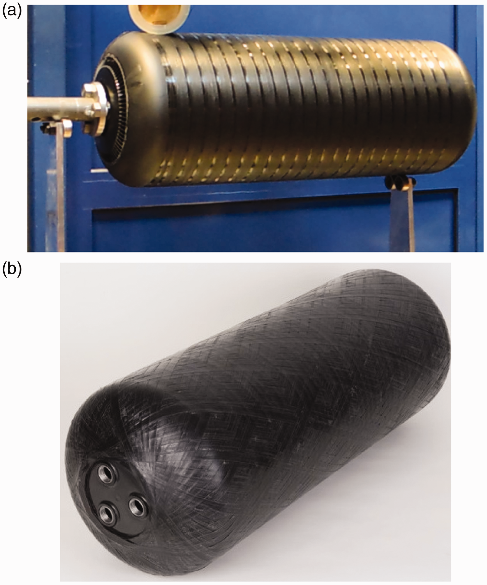

Temperature evolution and variation

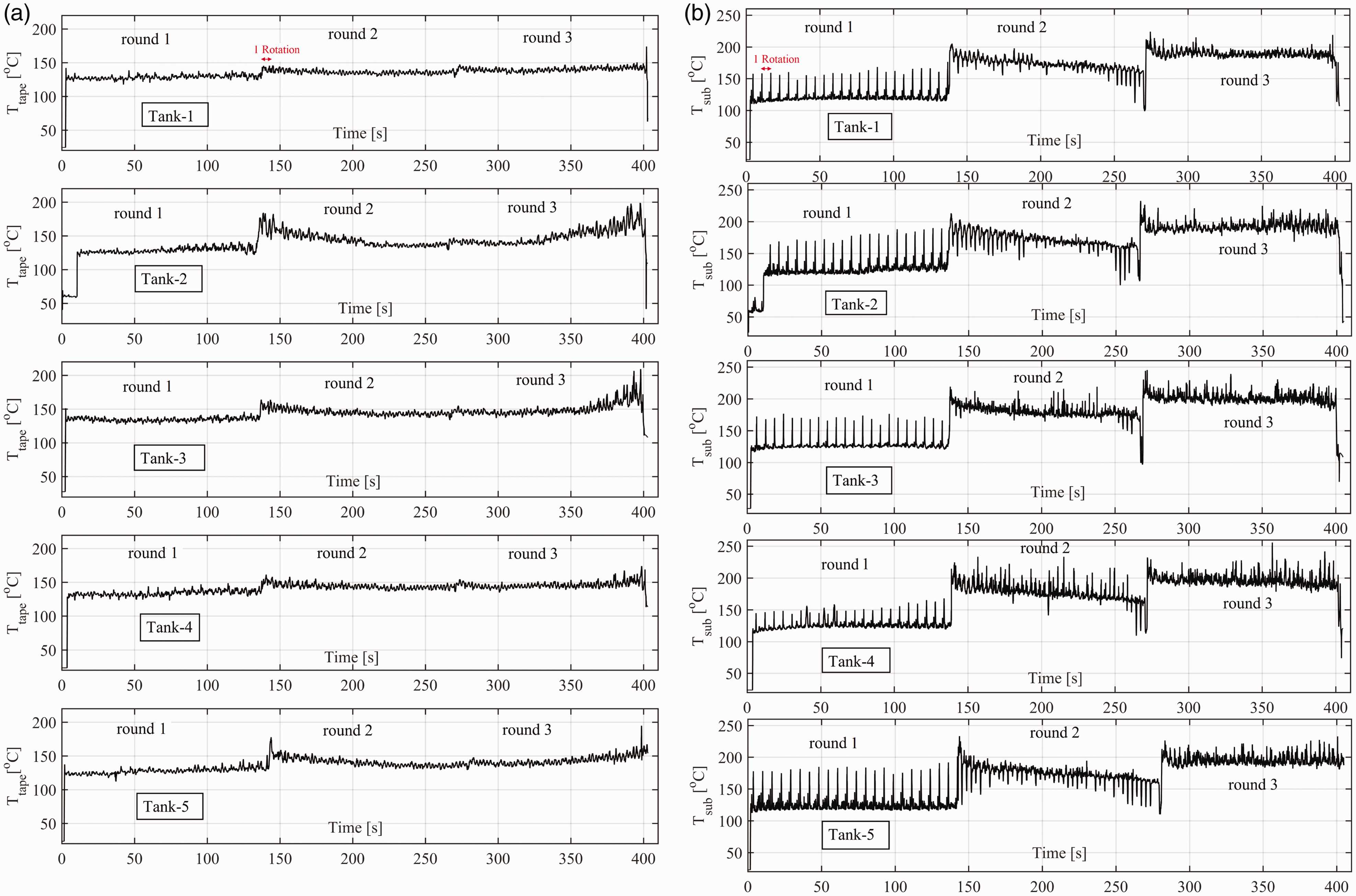
Five tanks were continuously wound with identical conditions. In all cases, the laser power was held constant during each round. The temperatures of the tape and the substrates were measured in a continuous fashion from the beginning to the end of the tape winding process, see Figure 9. In this figure, the temperature data of all tanks are shown for the tape and substrate. The following trends are visible for the temperature developments of all tanks:

Round 1: The substrate and tape temperatures showed an approximately constant baseline with a large number of spikes on top for the substrate. Over the whole range of the first round, the substrate temperature was about 10℃ lower than the tape temperature. The substrate and tape temperatures showed some degree of variation in temperature (±5℃) about the baseline along with the already mentioned positive spikes with magnitudes from 40℃ up to 80℃.

Round 2: The substrate temperature suddenly increased to temperatures about 75℃ higher than at the end of round 1, whereas the tape temperature only showed a minor increase of about 10℃. The substrate temperature in this round was always larger than the tape temperature. The substrate temperature showed a decreasing trend with the temperature dropping from 190℃ to 170℃, whereas the tape temperature decreased only a few degrees Celsius. The substrate temperature was showing much more variation in temperature than the tape temperature. The variation in the substrate temperature was comparable to that in round 1. In round 2, strong local variations in temperature occurred as well for all tanks, but both in the positive and negative direction.

Round 3: The tape temperature is changed hardly as compared to the previous round. The substrate temperature showed a strong increase at the start of round 3 of about 40℃, but it leveled off to an approximately constant value with a significant amount of variation. Also in round 3, strong local variations in temperature occurred.

Figure 9.

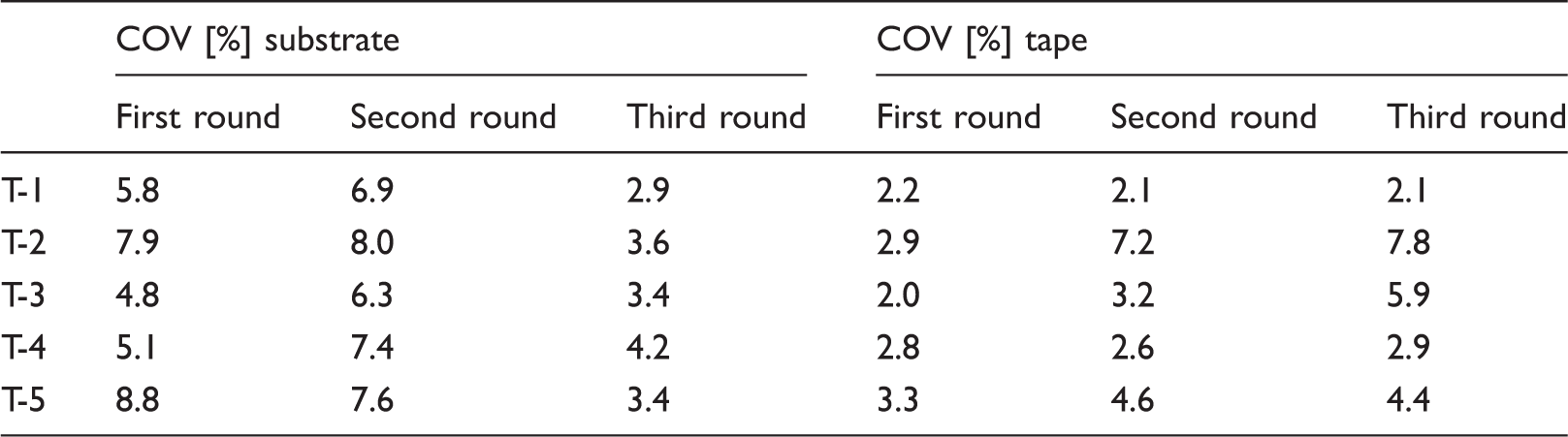
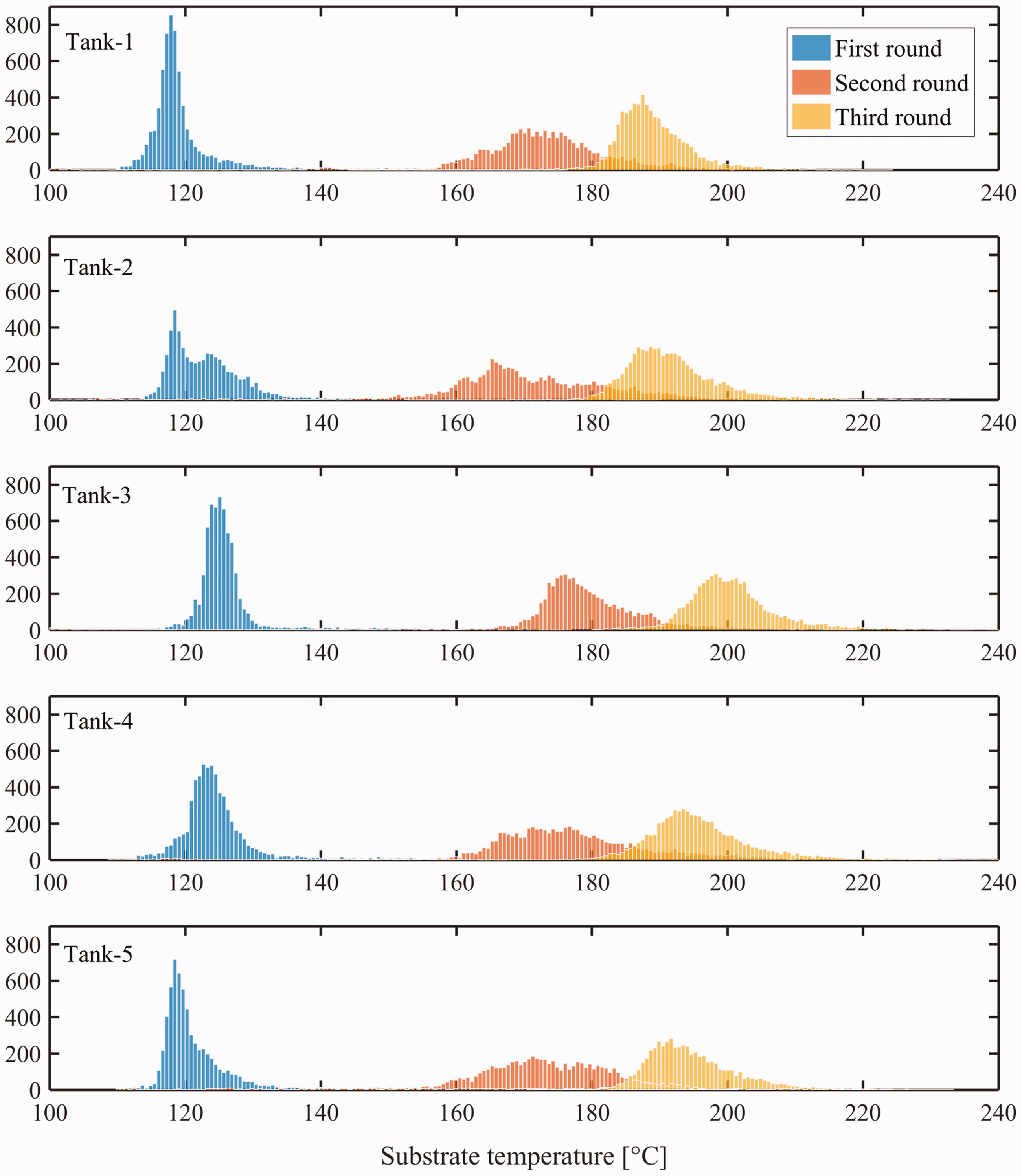
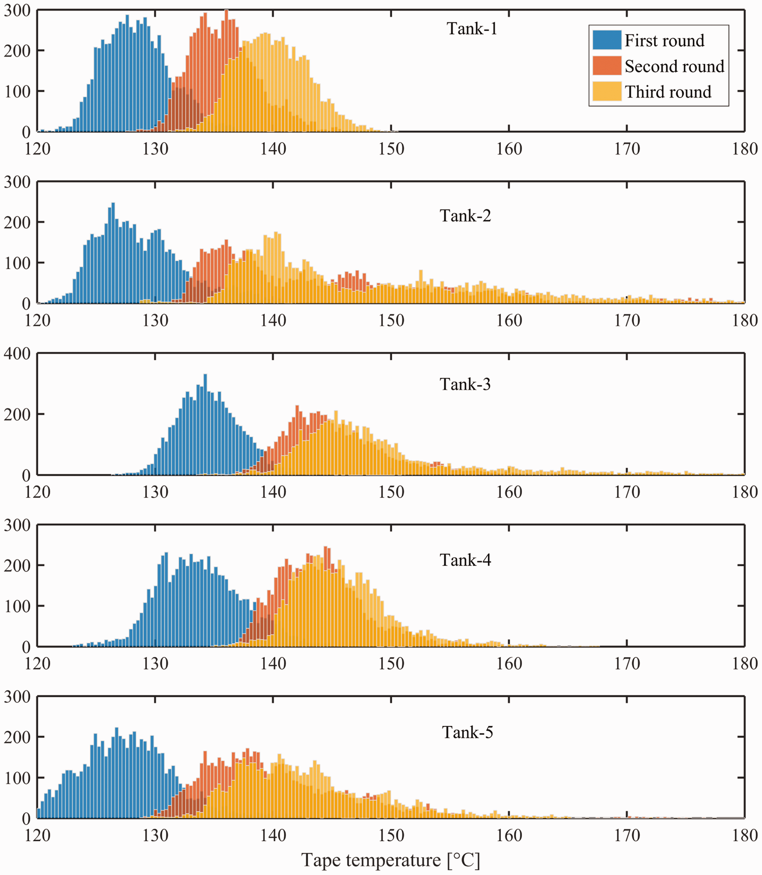
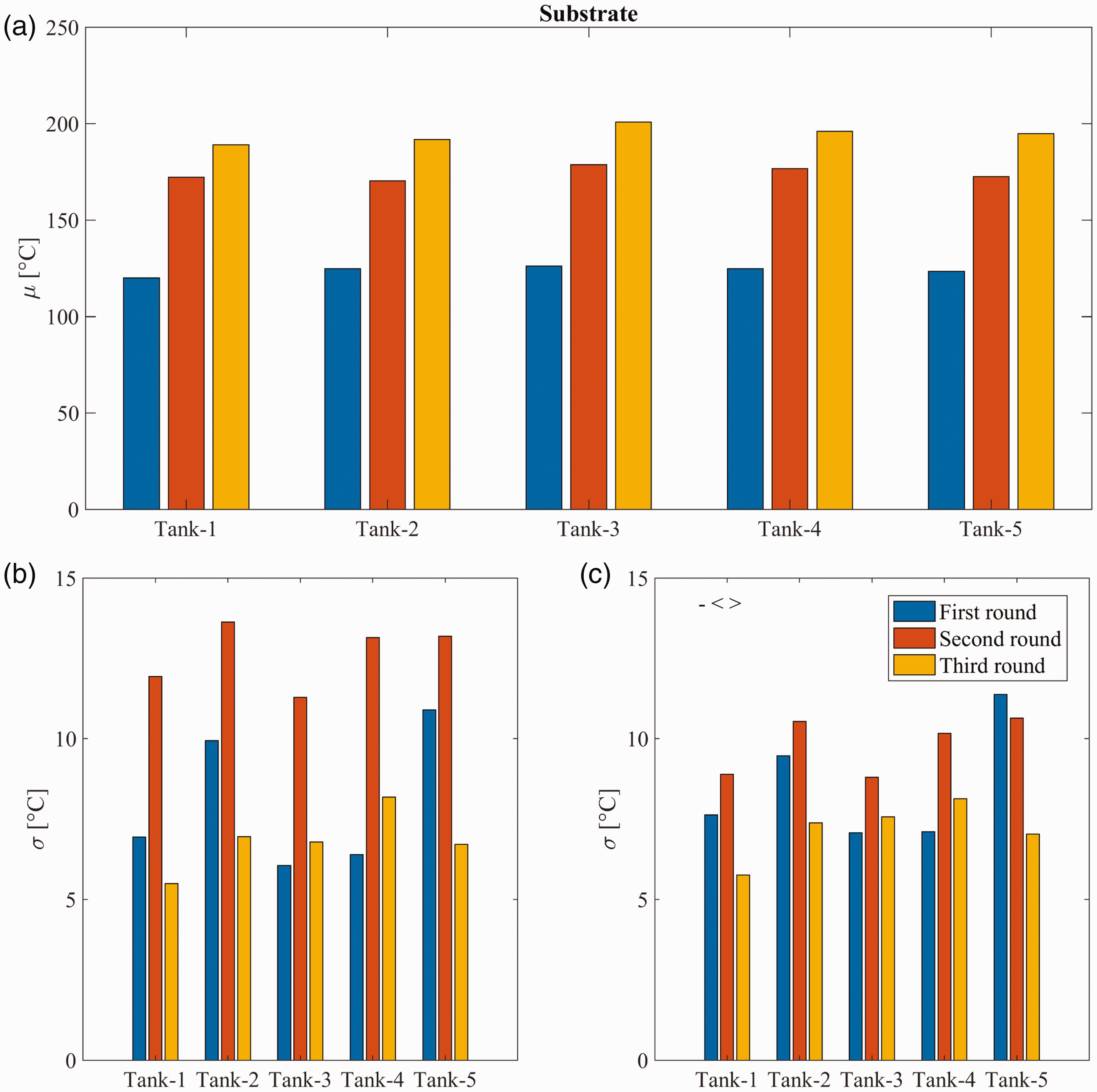
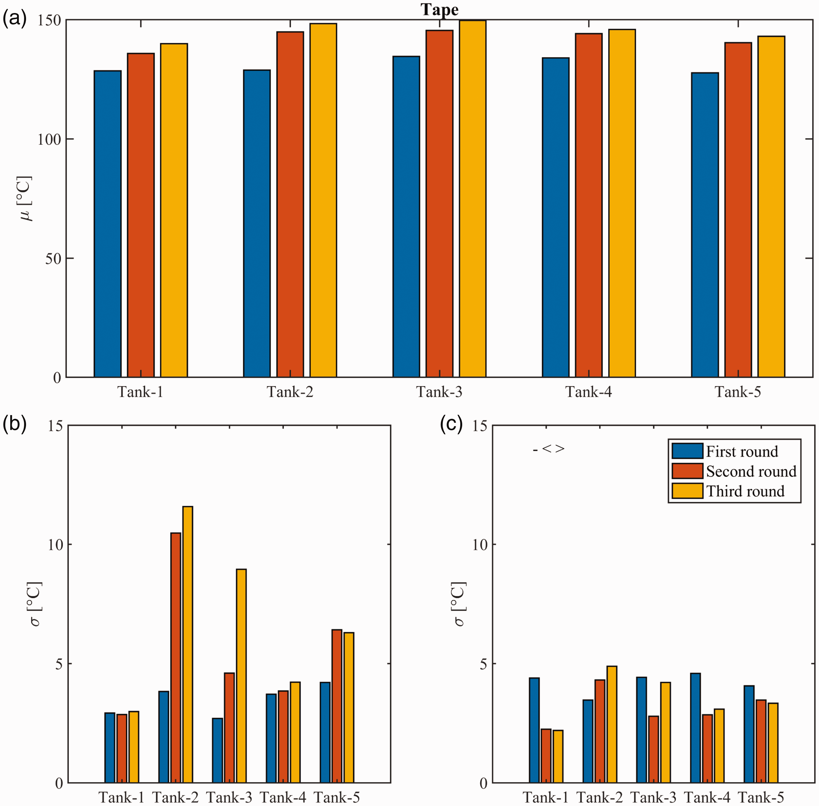
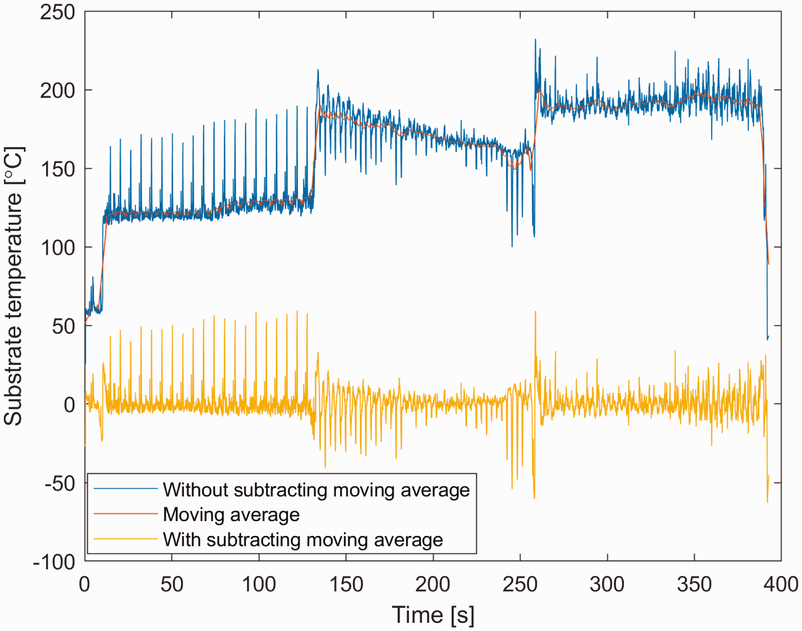
Tape (a) and substrate (b) temperature of three rounds adjacent hoop winding of five manufactured tanks via the LATW process. Each rotation takes roughly 6.2 s.

In order to quantify process variations, histograms of the measured process parameters were analyzed. The histograms of the temperature variation in the first, second and third round for each tank are illustrated in Figures 10 11 for the substrate and tape, respectively. The corresponding mean and standard deviation of the temperature distributions in each round are given in Figure 12 for the substrate and in Figure 13 for the tape. Here, the standard deviation was estimated with and without subtracting the moving average of the temperature evolution from the actual measurement. An example of the substrate temperature with and without subtracting the moving average temperature is depicted in Figure 14 for Tank-2. It is seen from Figure 12 that the mean substrate temperature increased gradually and was approximately 125℃, 175℃ and 195℃ for the first, second and third round, respectively. The standard deviation of the substrate temperature was approximately 8℃, 12℃ and 6℃ for the first, second and third round, respectively without subtracting the moving average. These values slightly decreased when the moving averages of the temperatures were subtracted. The increase in standard deviation from the first to second round and the decrease in standard deviation from the second to third round were consistent for the substrate and are discussed further in the following sections. A similar trend was observed for the mean tape temperature which was approximately 130℃, 142℃ and 145℃ the first, second and third round, respectively. The standard deviation of the tape temperature was in general smaller than the standard deviation of the substrate temperature with subtracting the moving average temperature. The coefficients of variation (COV) of the tape and substrate temperatures are depicted in Table 1. It is seen that the COV was 4.8–8.8% for the substrate temperature and 2.1–7.8% for the tape temperature. In the following, the observed trends based on the temperature evolution are discussed in more detail.

Table 1.

The coefficient of variation (COV = µ/σ) of the temperature variation in substrate and tape without subtracting the moving average temperature for tank liners represented as T-1 to T-5 (see Figure 9).

	COV [%] substrate			COV [%] tape
	First round	Second round	Third round	First round	Second round	Third round
T-1	5.8	6.9	2.9	2.2	2.1	2.1
T-2	7.9	8.0	3.6	2.9	7.2	7.8
T-3	4.8	6.3	3.4	2.0	3.2	5.9
T-4	5.1	7.4	4.2	2.8	2.6	2.9
T-5	8.8	7.6	3.4	3.3	4.6	4.4

Figure 10.

Histogram of the substrate temperature in the first, second and third round for all pressure tanks (for interpretation of the references to color in this figure legend, the reader is referred to the web version of this article).

Figure 11.

Histogram of the tape temperature in the first, second and third round for all the pressure tanks (for interpretation of the references to color in this figure legend, the reader is referred to the web version of this article).

Figure 12.

Substrate temperature: The mean (µ) (a), corresponding standard deviation (σ) without subtracting the moving average temperature (b) and standard deviation with subtracting the moving average temperature (c) for the first, second and third round.

Figure 13.

Tape temperature: The mean (µ) (a), corresponding standard deviation (σ) without subtracting the moving average temperature (b) and standard deviation with subtracting the moving average temperature (c) for the first, second and third round.

Figure 14.

The substrate temperature evolution for Tank-2 with and without subtracting the moving average. Length of moving average interval is considered as 1 s.

First round

At the start of the first round, the deposition head was placed closely to the tank liner and the tape is brought into contact with the liner. The liner was accelerated up to a nominal rotational velocity of about 140 mm/s. The laser was switched on as well and immediately started to heat up the tape and substrate. As long as the liner had not reached the nominal velocity, a slight overheating of the liner occurred which is visible as the first peak in tape and substrate temperatures at the start, see Tanks 1 and 5 in Figure 9. After the start of the process, the deposition head moved with a constant velocity parallel to the axis of the liner from the start position to the end of the liner. For Tank-2, the laser power was accidentally too low during a short period of time after the start explaining the relatively low temperatures. Similar phenomena related to a small degree of in-synchrony can also be observed at the end of round 3 when the tape winding process was stopped for some of the tanks.

Throughout the first round, the tape and substrate temperature remained more or less constant with distinctive peaks visible in the substrate temperature. Every time the laser irradiated the blow-molded edge part of the liner, which was formed during the blow-molding process of the tank liner (see also Figure 2), a temperature spike appeared. The number of spikes was identical to the number of rotations the tank made when covering the liner with a layer of tape during the first round as shown in Figure 9. The magnitudes of the peaks depended on the geometry of the blow molded edge such as the shape and height³² and therefore vary from tank to tank. The edge caused local energy concentration and hence sudden temperature elevations in the substrate temperature that may deteriorate the liner due to thermal and chemical degradation. Such excessive temperature values should be avoided in general.

During the first round, some variations in tape and substrate temperature were visible, apart from the observed spikes, that may be ascribed to variations in laser absorption of the liner and the tape as well as variation in material properties. Surface asperities and texture along with complex absorption mechanisms of the pure polymer pigmented HDPE tank and the glass fiber-reinforced HDPE tape can explain this behavior.^15,32,41

Second round

The second round started immediately after the first round with the tape winding head moving parallel to the liner axis in opposite direction from the end to the start position, while the liner continued to rotate with the same velocity (140 mm/s). At the beginning of the second round, sharp increases in the substrate temperatures were observed with high peak temperatures considerably above those at the end of the first round. There are two reasons explaining this observation. Firstly, the deposition process was continued in reverse direction while the substrate was still relatively hot from the deposition of the first layer. The laser power remained unchanged causing a significant increase in the substrate temperature. Secondly, the substrate material changed from a pure HDPE (liner) in the first round to a glass/HDPE composite, i.e. the deposited tape, in the second round affecting the amount of energy absorbed from the supplied laser irradiation.

During the deposition of the tape in round 2, the average substrate temperature showed a continuous decrease to approximately 160℃ at the end of the round 2 for all tanks. The temperature decrease was mainly caused by cooling of the substrate. After a point on the tank liner surface was covered by tape during round 1, it started to cool down from the process temperature of approximately 130℃. It depended on the amount of time for the tape winding head to move further to the end position and move back towards the start position how far the temperature may drop. The closer a point at the substrate was to the start position, the longer the time allowed for cooling and the further the temperature dropped in line with the observed substrate temperature development in round 2.

The apparently random peaks in the substrate temperature profile in the second round had a magnitude of smaller than 30℃. The reason of these peaks may be found in anisotropic reflections at the surface of the substrate due to non-ideal stacking of layers on top of each other causing local gaps in between tapes or overlap of adjacent tapes from the first round (see Schmitt and Witte²⁷ for gap/overlap and^42,43 for effect of laser reflection). This resulted in an increase in the COV and standard deviation in the second round as compared with the first round (see Figure 12 and Table 1). The origin of these local gaps and overlaps and other potential sources like fibers is discussed in the next section.

The tape temperature remained more or less constant with some scatter in between approximately 130℃ to 145℃ with a COV of 2.1–7.2%. Its mean value slightly increased with respect to the first round as seen from Figure 13 due to a larger scattering contribution from the substrate, which obtained a higher temperature during round 2 as compared to round 1. Another reason of increasing tape temperature at the beginning of this round especially for Tank-2 or Tank-5 is changing measurement location. This will be discussed in detail in the next section.

At the end of the second round, a sudden drop of the substrate temperature can be observed with a magnitude up to about 60℃. Here, the tape winding head moved beyond the starting point to a relatively cool part of the tank liner in the turning point between the second and the third round where no previously wound tape is present (uncovered part).

Third round

In the third round, the tape winding head moved again parallel to the liner axis from the start to the end position similar to the first round. The substrate temperature showed a strong peak at the beginning of the round for the same reason as it did at the start of the second round. The third layer was deposited on top of the second layer immediately after the second layer was deposited, so the substrate was still relatively hot while the laser power remained unchanged. Here, the temperature peaked at about 210℃ and during the third round it decreased to a fairly constant value of about 185℃. This value was mostly above the substrate temperature of the second round indicating a further heating of the substrate during the third round. Apparently, heat loss to the environment was not sufficient to keep the substrate from heating up which is also due to heating of the air enclosed within the tank liner.

On close inspection during the transition from the second round to the third round, a physically unrealistic drop in the substrate temperature was observed for all tanks with a magnitude of almost 100℃ at t = 270 s just before the temperature strongly increased. This drop was partly related to the tape being deposited on a relatively cold uncovered section of the tank liner, where no tape had been deposited before. The main reason, however, was that starting from the second round onwards, the emission coefficient of the tape was being used to interpret the thermal camera data of the substrate and illuminating uncovered liner material obviously led to wrong temperature data as the emission coefficient of the liner (0.6) differs from that of the tape (0.9), see also section “Materials and setup”. Although the tape temperature remained more or less constant with some scatter in round 3, the profiles of Tanks 2 and 3 showed a relatively steady increase of the tape temperature up to ∼50℃. As explained before, this behavior is related to the changing measurement location which will be elaborated in next section.

The COV and standard deviation of the substrate temperature decreased in the third round as compared with the second round as can be seen from Table 1 and Figure 12. This reduction in standard deviation can be due to the influence from the liner surface. The gap in between the deposited tapes was not as dominant in the third round as in the second round, i.e. the possible gaps between the deposited tapes in the third round consisted of the tape material instead of the pure HDPE liner as in the second round. At the end of the third round, a drop of temperature for both tape and substrate can be observed as the laser source is shut down. For some tanks prior to this temperature drop, a sharp rise in the tape and substrate temperature appeared, see for example Tank-1. This phenomenon was related to a small in-synchrony between shutting down the laser source and stopping the roller and tape movement.

Geometrical disturbances

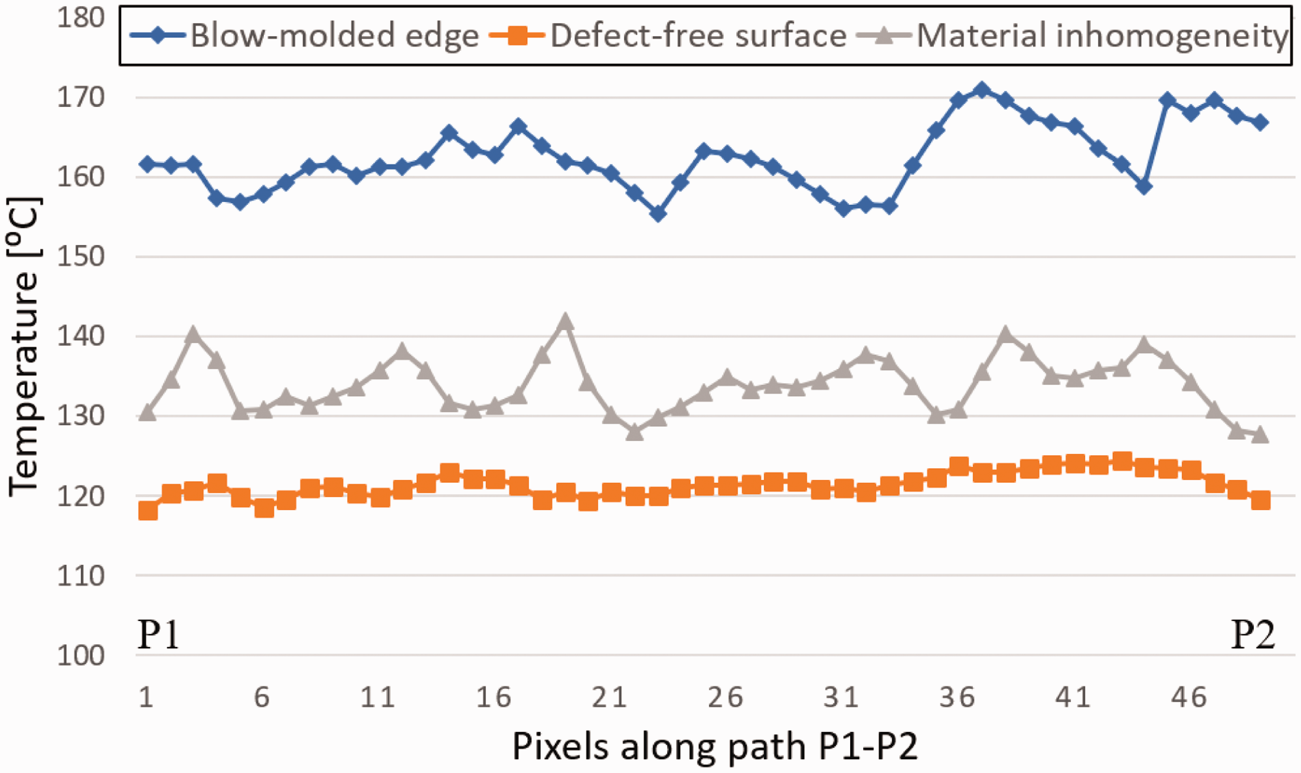
The highly localized substrate temperature spikes in the first round claimed due to the blow-molded edge were explored via the thermographic measurements. The exemplary thermographic snapshots in the first round showing polymer material inhomogeneity and blow-molded effects as well as defect-free surface of polymer liner are displayed in Figure 15. The increase of substrate temperature due to the blow-molded edge effects is in accordance with explanations in section “Temperature evolution and variation”. The temperature spike, i.e. the temperature increase, in Figure 15(c) due to blow molded edge was found to be approximately 43℃ as compared with the image shown in Figure 15(b). In order to quantify the temperature variation due to the aforementioned effects, a path was drawn in Figure 15 illustrated as a line from point P1 to point P2. The temperature variation along the path P1–P2 is plotted in Figure 16. It is seen that the temperature was approximately 120℃ for the defect-free case with a slight variation. The material inhomogeneities of the polymer liner caused an increase in the mean temperature which was approximately 135℃ and its variation was found to be approximately 10℃. The change in surface topology and roughness might have caused this increase and variation in the substrate temperature. The blow-molded edge had the most influencing effect where the mean substrate temperature reached approximately 165℃ with a maximum value of approximately 170℃. The blow-molded edge can be considered as locally a rough area where the laser irradiation was localized and hence resulted in a sharp increase in the temperature.

Figure 15.

Thermographic images of the irradiated area near the nip-point in the first round. (a) No edge/ material inhomogeneity (defect-free surface), (b) effects of material inhomogeneity and (c) blow-molded edge of the polymer liner (substrate in first round) are displayed. The path P1–P2 is drawn in the width direction of the substrate to get quantitatively variation of the temperature due to the mentioned effects (for interpretation of the references to color in this figure legend, the reader is referred to the web version of this article).

Figure 16.

Temperature variation of path P1–P2 in the first round due to the material inhomogeneity and blow-molded edge of the polymer liner as well as defect-free surface which are represented graphically in Figure 15.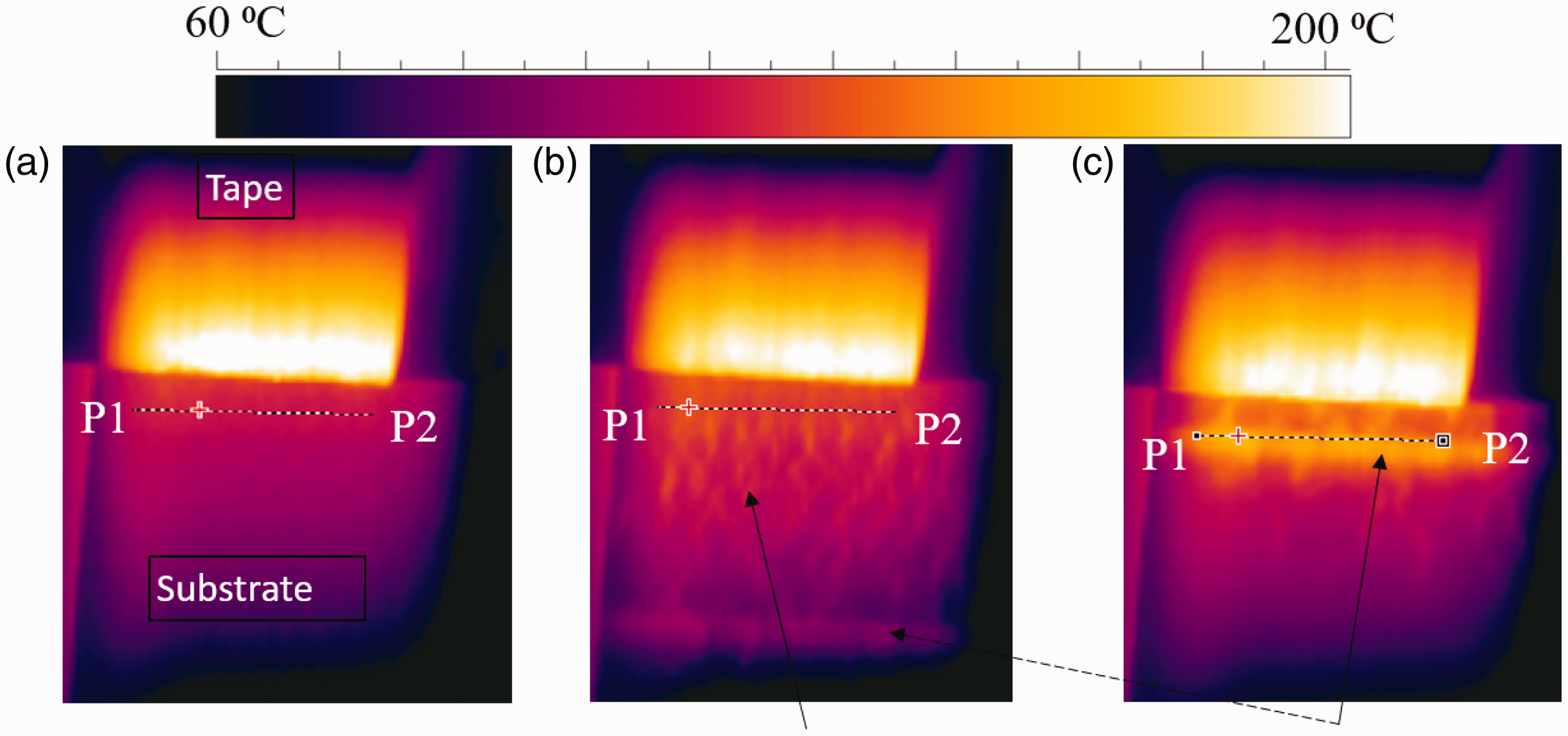

Another possible geometrical disturbance was the eccentricity which caused a non-uniform liner movement and hence affected the location at which the thermal camera measurements were recorded. This is illustrated for Tank-2 in Figure 17 in which three different locations for the measurement box for substrate, tape and nip point are shown. It should be noted that the movement of the measurement box is present only when there is an eccentricity. As a consequence, the change in tape temperature due to the movement of the measurement box was obtained approximately as 44℃ according to the frames shown in Figure 17 which was aligned with the increase in tape temperature for Tank-2 as shown in Figure 9.

Figure 17.

Thermographic images of the irradiated area near nip-point in the second round indicating the movement of the thermal camera measurement targets at tape, nip point and substrate. (a) Correct measurement location, (b) upward and (c) downward movement of the measurement locations due to the unavoidable eccentricity (for interpretation of the references to color in this figure legend, the reader is referred to the web version of this article).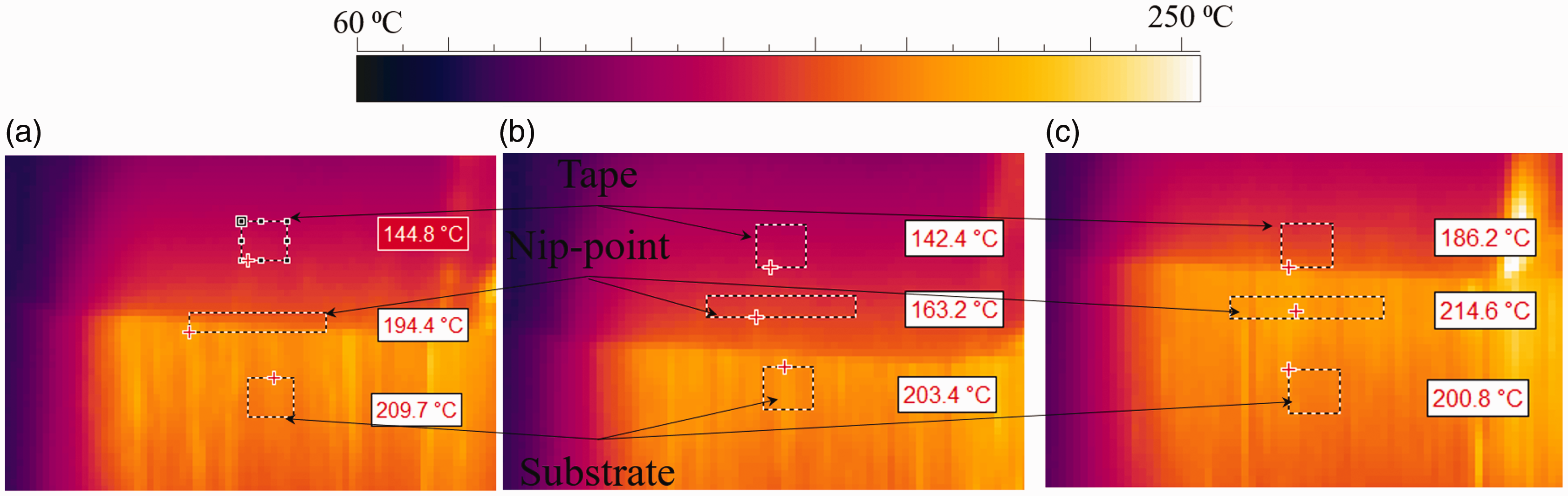

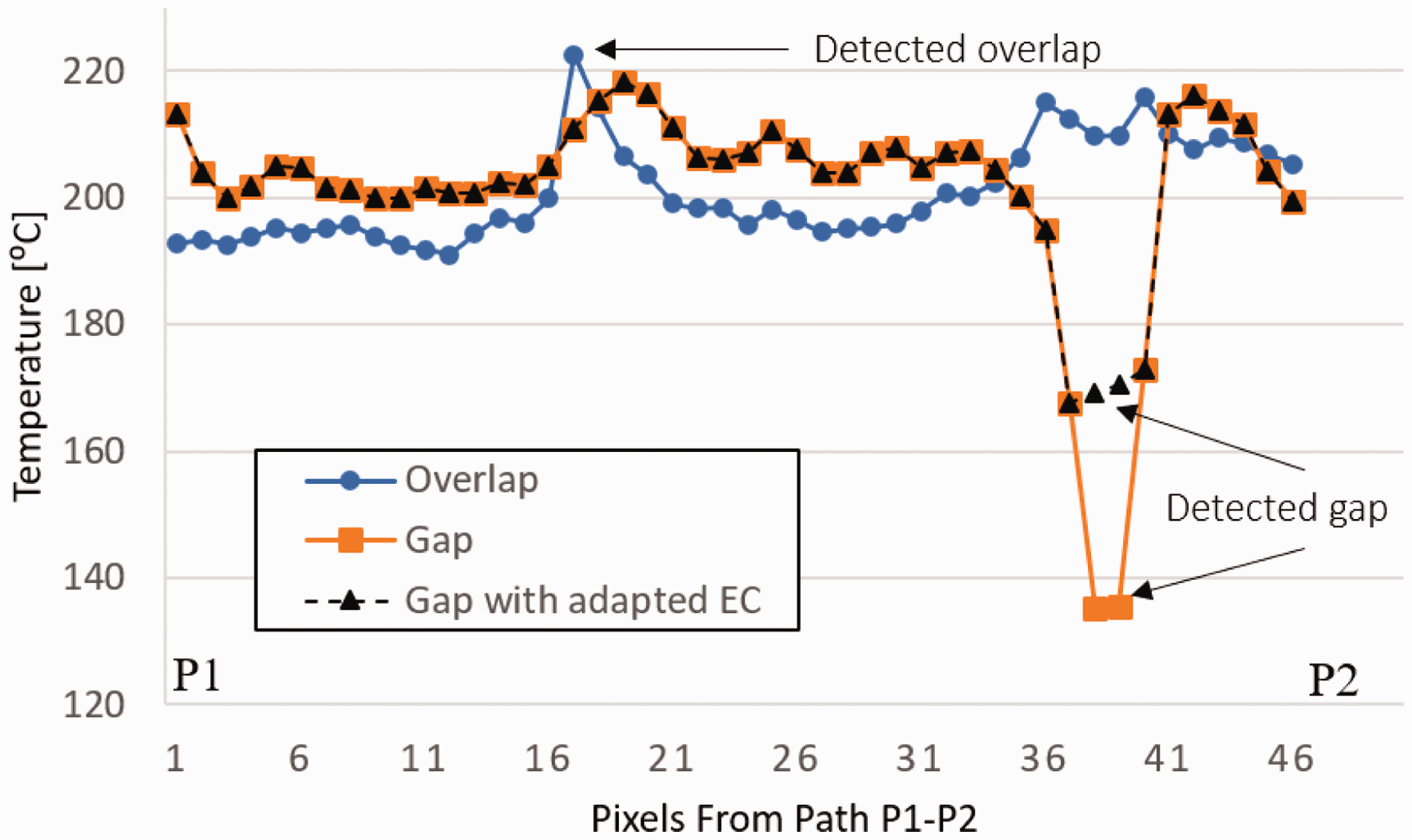
The gap and overlap formations were captured using the thermographic images which are displayed in Figure 18. The origin of these regions with gaps/overlaps lied in the non-ideal shape of the liner (being slightly unround during tank liner production or deformation due to exerted roller force) and the unwanted eccentric fixation of the liner on the tape winding device. These local features caused a variation in the temperature measured by the thermal camera mainly due to the change in the local geometry which affected the heat absorption and laser light reflection locally. In addition, the emission coefficient used in the thermal camera needed to be updated with respect to the local geometry which was not the case during the experiments. To illustrate, in the case of gap during the second round, the HDPE liner material was visible for the camera, which caused a lower temperature recorded by the camera. On the other hand, in the case of an overlap, the laser irradiation was localized providing a sharp increase in substrate temperature. At this situation, the emission coefficient needed to be lowered at this time frame due to high temperature (see Appendix for the variation in emission coefficient with respect to the temperature). The path P1–P2 defined in Figure 18 was used to quantify the temperature variation at the gap/overlap regions. The temperature variation profile along P1–P2 path (extracted from pixels) is shown in Figure 19. The locations of the gap/overlap in the temperature profiles were related to the pixels containing the gap/overlap in the thermographic images. The emission coefficient (EC) of the pixels (pixels 37–39) with gap was adapted manually with correct value from the polymer liner in order to show the influence of this effect. The temperature dropped from approximately 210℃ to 135℃ due to the gap. By adapting emission coefficient to 0.6 (was 0.9) for the pixels constituting the gap, the corrected temperature was estimated approximately as 170℃ due to the gap as seen in Figure 19. On the other hand, the substrate temperature increased to approximately 235℃ due to the overlap.

Figure 18.

Thermographic images of the exemplary (a) gap and (b) overlap in the second round which causes localization of the substrate temperature. The path P1–P2 is drawn in the width direction of the substrate to get quantitatively the maximum (shown in the pictures) and variation of the temperature due to the gap/overlap effects (for interpretation of the references to color in this figure legend, the reader is referred to the web version of this article).

Figure 19.

Temperature variation of path P1–P2 in the second round due to the gap and overlap of wound tape (substrate) is represented graphically in Figure 18. Manually adapted emission coefficient (EC) of the gap region is also added.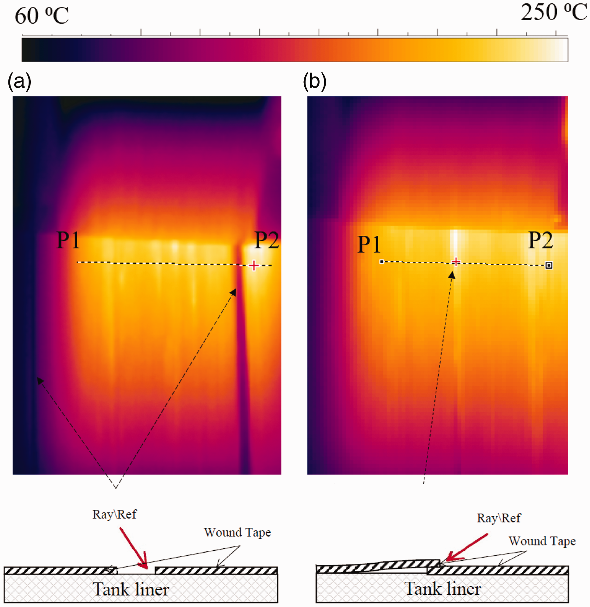

In order to evaluate the temperature variation excluding the gap/overlap on the substrate, e.g. during the second round, a total of 50 images which did not include the gap/overlap were selected randomly at different time stamps. The temperature variation along P1–P2 path was analyzed for each thermal image and plotted in Figure 20. Total of 25 pixels were considered on P1–P2 path. The mean average of the temperature along P1–P2 path was subtracted from the temperature profile along the path P1–P2 in order to quantify the measured temperature variation due to a possible material homogeneity. The temperature values for each pixel along the path P1–P2 were grouped for the 50 images and represented as a box and whisker plot in Figure 20. This chart shows distribution of data into quartiles, highlighting the mean, median and outliers. The boxes, which represent 50% of the data set, have the lines extending vertically called “whiskers”. These lines indicate variability outside the upper and lower quartiles of the observations, and any point outside those lines or whiskers is considered as an outlier. The mean is marked as central cross and median is shown by a horizontal line inside the box as shown in Figure 20. Approximately 5℃ variation (length of boxes) was observed as a general trend for each pixel. The most of the outliers were observed approximately as 10℃ and few of them were found to be approximately 25℃. The outliers with high scatter might be due to a possible nonuniformity of the fiber distribution or the change in orientation of the material surface (see Appendix 1 for the variation of emission coefficient with respect to the thermal camera angle).

Figure 20.

Box and whisker plot representing temperature variation at indicated pixels (path P1–P2 in the width direction of the substrate) for randomly selected 50 frames images. Note that the images containing edge effect/gap/overlap are excluded in the selection procedure and the mean average of the temperature along P1–P2 path was subtracted.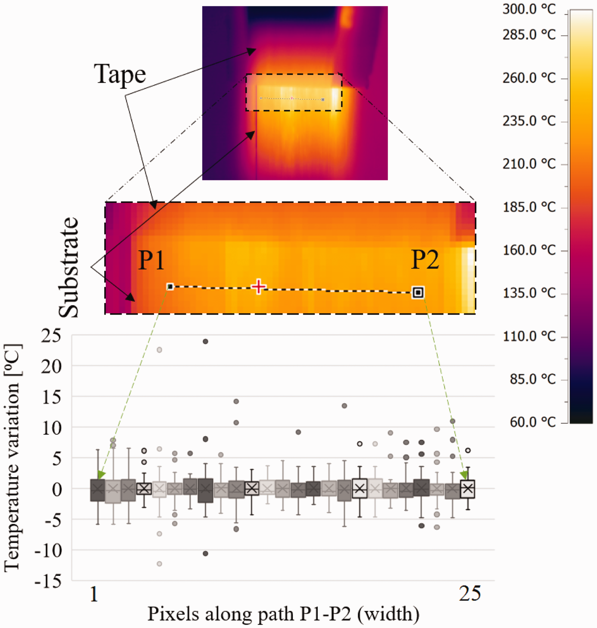

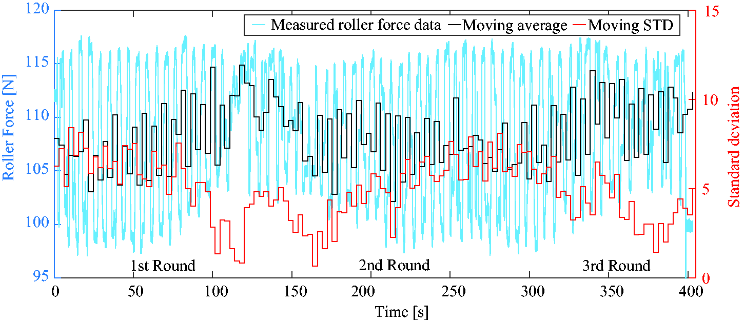
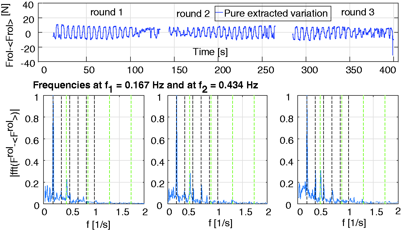
The periodical vertical change in the nip-point position can be determined by analyzing the roller force distribution for each round which can be seen in Figure 21. It is seen that much random scatter was the case for all the rounds as compared with the tape and substrate temperature distributions seen in Figures 10 and 11. Although the nominal roller force was set to 105 N, roller force clusters were observed relatively lower and higher force values, e.g. 97 N and 117 N for Tank-2; 102 N and 118 N for Tank-3; 106 N and 115 N for Tank-5. These clustering of the roller force clearly indicate a periodicity in the liner response with respect to the exerted roller force. To illustrate, the development of the roller force during the tape winding process of Tank-2 is displayed in Figure 22. During most of the first round, the mean and standard deviation of the roller force were more or less constant for Tank-2; however, towards the end of round 1 the mean value increased and the standard deviation decreased. In round 2, the mean value reduced to a more or less constant value similar to that in the first part of round 1 and this value was also maintained in the first half of round 3. In the second half of round 3, an increase in the mean roller force was observed with a concomitant reduction of the standard deviation. The locations of these changes at the end of the first and third round are related to a relatively large stiffness at the dome part of the tank (the right side of tank liner in Figure 7) where the cylindrical part of the tank liner is supported by two bearings. Fluctuations in the roller force were caused by changes in the vertical position of the consolidation roller, as can be learned from Figure 4, where the spring/damper construction attached to the consolidation roller is displayed. The roller force oscillations in Tank-2 were analyzed through a Fourier analysis of the force-time signal in Figure 23. Here, the relative magnitudes of the signals as a function of the frequency are displayed for the three rounds, where the data at some distance from the start and end positions were selected (in order to eliminate the effect of transition parts between rounds). In line with the repetitive nature of the roller force oscillations, distinctive peaks in frequencies can be observed that can be related to the tape winding process. The first peak at a frequency of about 0.16 Hz corresponds to a periodic signal with a period of 6.2 s, which exactly corresponds with the time it takes for the tank liner to make a revolution. The other peaks may be regarded as higher orders or can be related to other periodic signals. For example, the signal at 0.43 Hz can be related to the time it takes for the consolidation roller to make a revolution. On closer inspection, indeed the roller showed some geometrical inconsistencies that could very well explain the presence of this signal. Hence, the observed variations in the roller force can directly be related to the rotational nature of the tape winding process. The local variations in liner diameter related to unroundness and excentricity can lead to the formation of small gaps and regions with some tape overlap due to the trajectory change. In turn, the regions with gaps/overlap may cause irregular reflection/absorption behavior of the laser rays leading to different substrate temperature values, both above and below typically expected values. This largely explains the substrate temperature variation in the second and third round (see Figures 9, 10 and 12).

Figure 21.

Histogram of the roller force in the first, second and third round for all the pressure tanks (for interpretation of the references to color in this figure legend, the reader is referred to the web version of this article).

Figure 22.

Measured roller force data (total number of measured data is ∼400 K) and moving average value and corresponding standard deviation (STD) of Tank-2 for round 1, 2, 3. Interval of 5 s for moving mean values was chosen in order to show clearly overall trend.

Figure 23.

Discretized pure variation vs. time (top figure) of Tank-2 obtained by subtracting the moving average values (<Frol >) from the original ones (Frol) in round 1, 2, 3. The Fourier analysis (blue lines in bottom figure) of roller force (fft(Frol- <Frol >)) along with dominant frequencies at f₁ = 0.167 Hz (black dashed lines) and f₂ = 0.434 Hz (green dashed lines) for each round are calculated. Other vertical lines indicating factors of f₁ and f₂ are also shown as vertical black dashed line and green dashed line, respectively.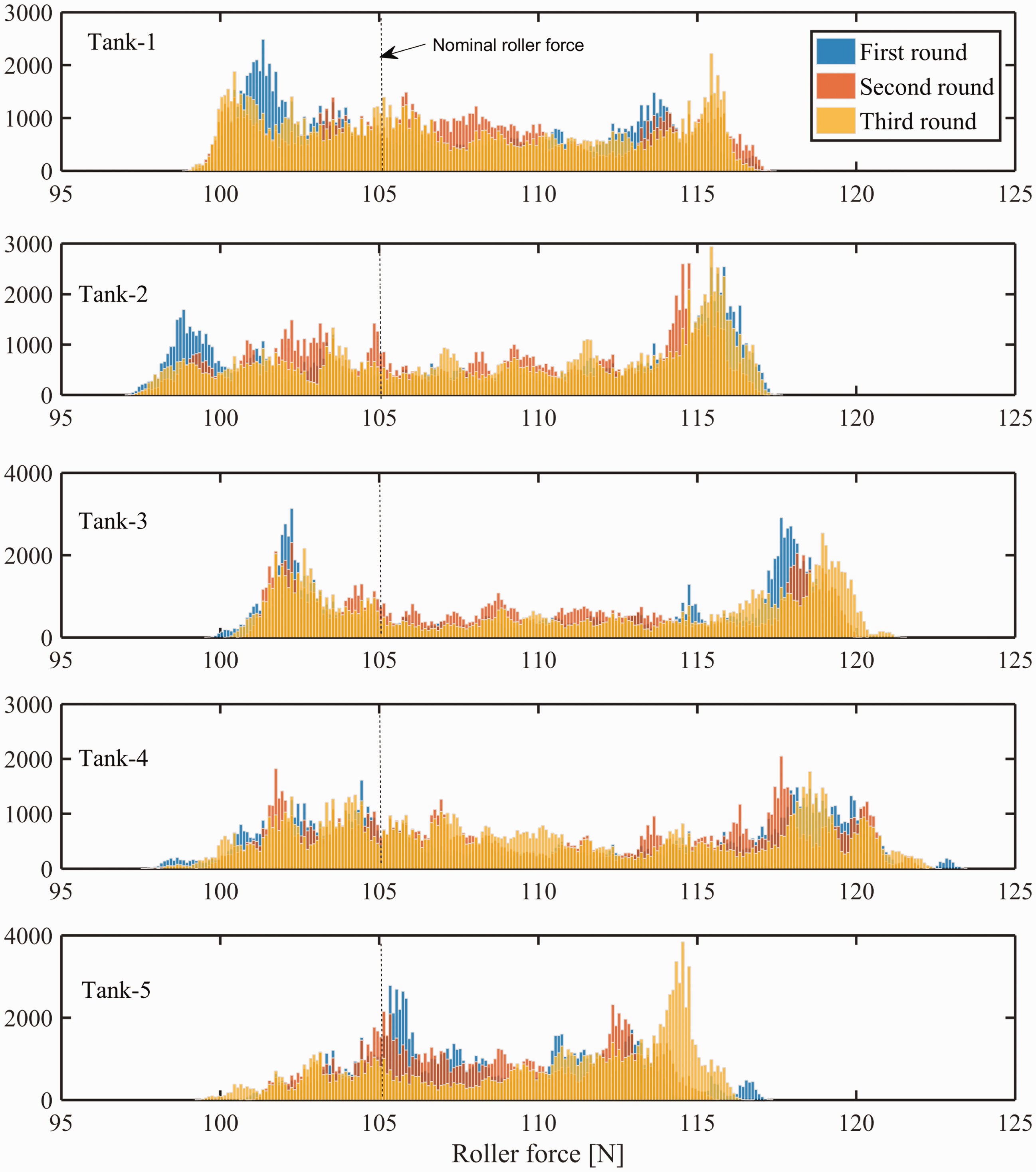

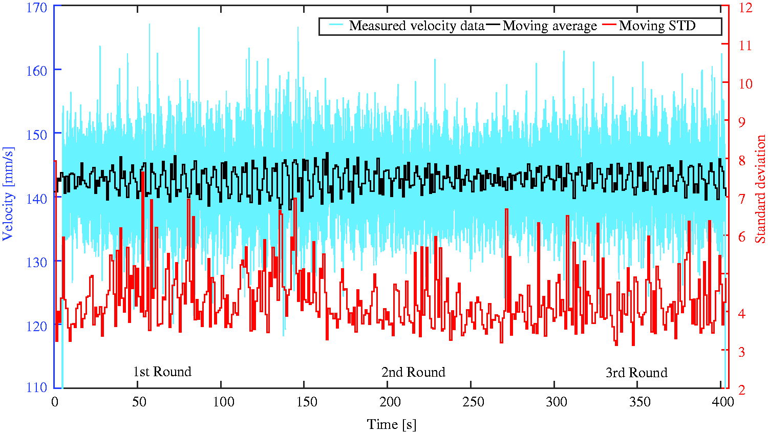
In addition to the roller force, the tape feeding velocity was also affected by the geometrical disturbances, i.e. the unroundness and eccentricity. The histogram of the tape feeding velocity for each round is shown in Figure 24. It is seen that the velocity distribution trend was almost the same for each round and the distribution was very close to the normal distribution where the nominal set value was 140 mm/s. The mean and standard deviation of the measured velocity were approximately 143 mm/s and 5 mm/s, respectively. To illustrate, the measured velocity data, moving average values and moving standard deviation of adjacent hoop-winding for Tank-2 are shown in Figure 25. The variation of measured linear velocity is roughly 10 mm/s with some spikes that amounts to 20 mm/s.

Figure 24.

Histogram of the tape feeding velocity in the first, second and third round for all the pressure tanks (for interpretation of the references to color in this figure legend, the reader is referred to the web version of this article).

Figure 25.

Oscillation in measured tape feed velocity of thermoplastic pressure vessel Tank-2 via LATW process. The total number of measured data is ∼400 K. The moving average and standard deviation (STD) of the measured velocity are also depicted. Interval of 5 s for moving mean values was chosen in order to show clearly the overall trend (for interpretation of the references to color in this figure legend, the reader is referred to the web version of this article).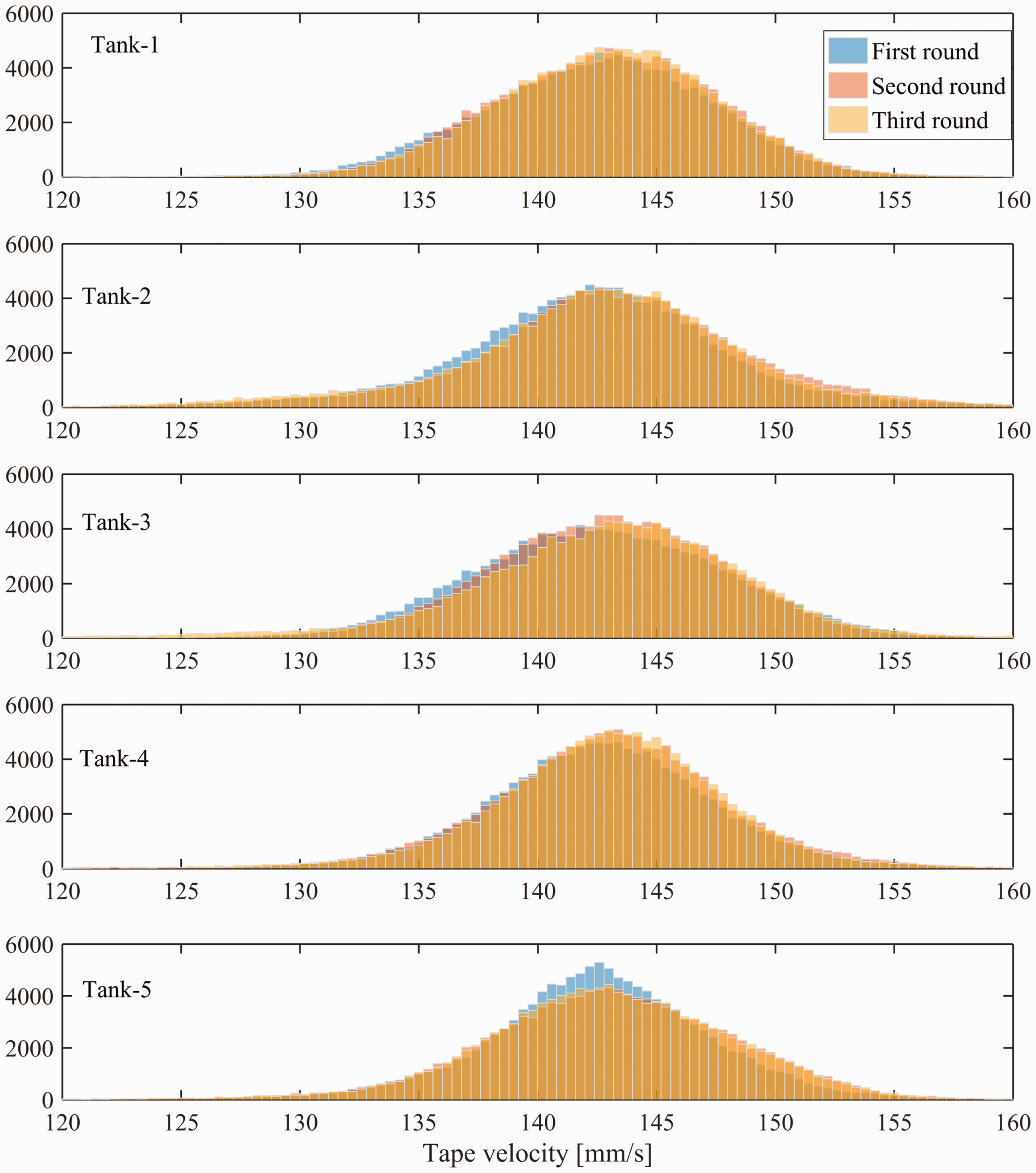

A Fourier analysis of the tape feeding velocity, temperature of tape and substrate data was conducted in a same manner as the roller force analysis which is shown in Figure 26 for Tank-2. The same dominant frequencies observed from the analysis of the roller forces are observed for the tape and substrate temperature deviations providing strong evidence that the variations in the roller force and both temperatures were linked. The unroundness and eccentricity also caused variations in the required supply speed of the tape that was deposited on top of the tank liner and the tape tension. The actual supply speed is equal to the tangential velocity at the nip-point which in turn is dependent on the local value of the tank liner diameter. Unroundness and eccentricity cause temporal variations in the diameter and, in turn, in the required supply speed. As the laser source supplies a constant power, the heating rates of the tape may temporarily change, depending on the tape speed. The larger the local tape speed, the smaller the temperature increase of the tape at constant laser power. This also holds to some extent for the substrate surface heated by the laser source. A Fourier analysis of the tape speed, carried out in the same way, indeed shows that the frequencies present in the tape temperature, substrate temperature, tape tension and roller forces can explain the speed variations observed, see Figure 26 for the results of the analysis of Tank-2.

Figure 26.

Fourier analysis (blue color) of: (a) velocity, (b) tape temperature and (c) substrate temperature of Tank-2 along with dominant frequencies at f₁ = 0.167 Hz (black dashed lines) and f₂ = 0.434 Hz (green dashed lines) in round 1, 2, 3 are calculated. Other vertical lines indicating factors of f₁ and f₂ are also shown as vertical black dashed line and green dashed line, respectively. Note that the Fourier analysis was applied to the values where the moving average was subtracted from the original values, i.e. for the tape velocity fft(Vtape- <Vtape >), for the tape temperature fft(Ttape- <Ttape >) and for the substrate temperature fft(Tsub- <Tsub >).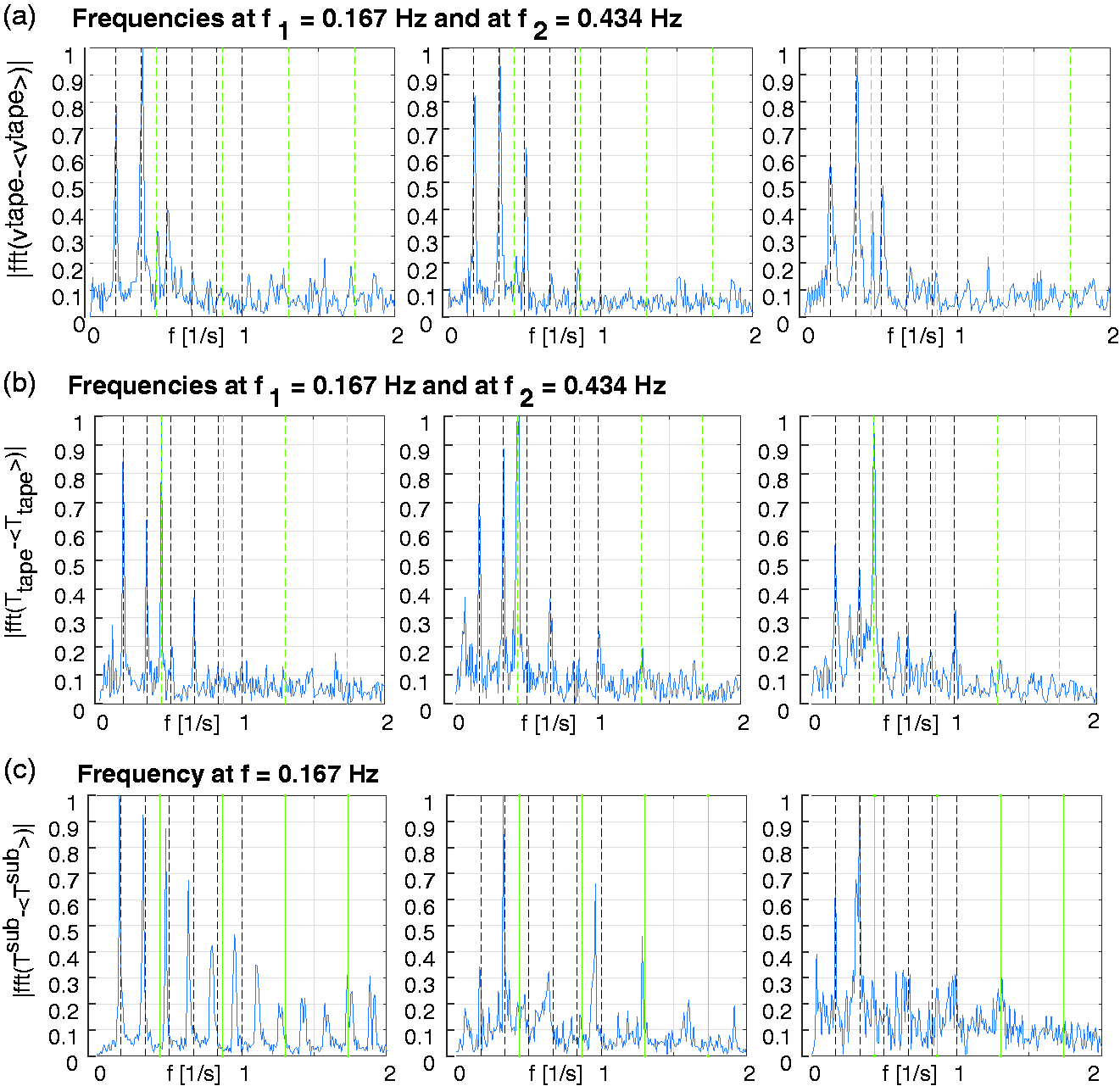

Process improvement

The laser-assisted adjacent hoop winding of three rounds on a tank liner at constant laser power can be done well but led to significant changes in the process temperature during the deposition process. The optimal and well-controllable conditions should be achieved during the tape winding process for the superior manufactured product. As observed from the results presented in this work, such ideal manufacturing conditions due to the geometrical disturbances cannot be established. Therefore, suitable approaches should be developed to control the temperature evolution globally and locally as well as fluctuations in temperature due to geometrical disturbances. This is necessary to optimize the final part properties with a better understanding of the thermal history of the material.

Although the feedback temperature controller seems to be a solution to ascertain a constant nip-point temperature, it is not sufficient for process control when the disturbances like measurement location movement or gap/overlap exist. Therefore, there is a need to detect the geometrical disturbances and adapt the thermal camera measurements accordingly, e.g. the measurement location and emission coefficient of the thermal camera. A potential solution for this is the real-time object detection technique using the deep-learning methods such as RCNN, YOLO or SSD.^44–46 This can be integrated into the LATW system. The real-time object detection can also be used for realizing gap and overlap where the emission coefficient is changing. At these locations, thermal camera should use different emission coefficient to measure the right temperature. Adapting laser power for the desired temperature at those regions needs such a laser-like VCSEL laser (see Weiler et al.²²) which could precisely adjust its power toward the gap/overlap regions. Integrating physics-based in-line monitoring model is also another possibility to create such model predictive control model, i.e. those developed in Montazeri-Gh et al.,⁴⁷ in order to interpret the actual temperature and control it for the LATW application.

Conclusion

In this work, laser-assisted tape winding was used to manufacture a number of type-IV thermoplastic composite pressure vessels. A constant laser power was employed during continuous adjacent deposition of three layers of a glass-filled HDPE thermoplastic fiber tape on an HDPE liner. The development of the substrate and tape temperatures along with other key characteristics of the deposition process was analyzed in detail for a reliable manufacturing. In addition, the variation in tape and substrate temperature was quantified. The following conclusions can be drawn.

Applying a constant laser power while depositing layers of tape on top of each other in a continuous adjacent fashion leads to a non-constant process temperature. The process temperature is sensitive to the average substrate temperature that in turn is dependent on the local heating and cooling cycles induced by the LATW process. Continuing the tape winding process directly after the deposition of the first layer causes a significant increase in the average substrate temperature. The mean tape and substrate temperatures were found to increase approximately by 12℃ and 50℃, respectively, from the first round to the second round. The temperature change can be attributed both to the change in substrate material (from a bare liner to a first layer of tape on a liner) as well as to the heat accumulated in the first round. Heat accumulation also led to an increase of the average tape and substrate temperature of around 3℃ and 20℃, respectively, from the second round to the third round.

The mean temperature of the substrate and tape temperatures increased gradually round by round. However, the trend of the COV and standard deviation was found to be non-linear due to the process disturbances. A larger COV of the substrate temperature (4.8–8.8%) than the COV of tape temperature (2.1–7.8%) was found from the histograms of measured temperatures. The standard deviation of the substrate temperature in the third round was found to be smaller than the second round.

The detailed analysis conducted in this paper showed the importance of the relation between process parameters and geometrical anomalies (surface features, eccentricity, unroundness) that have a severe impact on the actual and/or measured temperature in the process zone. Even the presence of a small blow molded edge may cause a significant increase in the temperature as observed during the tape winding in the first round via the thermographic images.

This blow molded edge effected the periodic scatters in the first round of adjacent hoop winding with an amount of 20–50℃.

Eccentricity and unroundness of the tank liner caused variations in tape velocity, substrate and tape temperatures which generated reaction forces by the roller as shown through detailed Fourier analysis.

Moreover, the unroundness and eccentricity were found to be the potential reason for the change in measurement location and the occurrence of gap/overlap. The locations on the tank surface with gaps between the deposited tape and overlap of adjacent layers led to considerable local temperature variations during the second and third round. The overall temperature variation was found to be approximately ±5℃ for the randomly selected 50 thermal images for the substrate in which the gap and overlap features were excluded.

The quantified temperature variations might not be critical to generate unwanted degradation. Nevertheless, they may affect the local temperature history of the material, e.g. the cooling rate and the temperature at consolidation may differ, which drives the mechanical property evolution via crystallinity, residual stresses, etc. It is therefore vital to understand, describe and quantify the variation in temperature during process which would pave the road towards developing more robust inline control strategies. In addition, a well described inherent temperature variation could help the composite structure designers to make more reliable product designs by taking the possible variations in the thermal history, e.g. the quantified COV data per round, and using it in a stochastic analysis.

Monitoring disturbances with thermographic images and Fourier analysis, it was concluded that a real-time adaptive detection of the nip-point location needs to be employed together with a feedback temperature control system in order to take the temperature variations due to geometrical disturbances into account.

Supplemental Material

JCM884101 Supplemetal Material - Supplemental material for Temperature variation during continuous laser-assisted adjacent hoop winding of type-IV pressure vessels: An experimental analysis

Supplemental material, JCM884101 Supplemetal Material for Temperature variation during continuous laser-assisted adjacent hoop winding of type-IV pressure vessels: An experimental analysis by Amin Zaami, Martin Schäkel, Ismet Baran, Ton C Bor, Henning Janssen and Remko Akkerman in Journal of Composite Materials

Footnotes

Acknowledgements

The dissemination of the project herein reflects only the author’s view and the Commission is not responsible for any use that may be made of the information it contains.

Declaration of Conflicting Interests

The author(s) declared no potential conflicts of interest with respect to the research, authorship, and/or publication of this article.

Funding

The author(s) disclosed receipt of the following financial support for the research, authorship, and/or publication of this article: ambliFibre project has received funding from the European Union’s Horizon 2020 research and innovation programme under grant agreement No 678875.

References

Njuguna

. Lightweight composite structures in transport: design, manufacturing, analysis and performance, Cambridge, UK: Woodhead Publishing, 2016.

Weisberg

Aceves

Espinosa-Loza

, et al. Cold hydrogen delivery in glass fiber composite pressure vessels: analysis, manufacture and testing. Int J Hydrogen Energy 2013; 38: 9271–9284.

Ramirez

JPB

Halm

Grandidier

J-C

, et al. 700 bar type IV high pressure hydrogen storage vessel burst-simulation and experimental validation. Int J Hydrogen Energy 2015; 40: 13183–13192.

Farhood NH, Karuppanan S, Ya H, et al. Advanced materials for sustainability and growth. In: Proceedings of the 3rd Advanced Materials Conference 2016 (3rd AMC 2016), Langkawi, Malaysia, 28–29 November 2016, Melville: AIP Publishing, 2017.

Red

. Pressure vessels for alternative fuels, 2014-2023. Compos Technol 2014; 20: 22–27.

Neto

Chludzinski

Roese

, et al. Experimental and numerical analysis of a lldpe/hdpe liner for a composite pressure vessel. Polym Test 2011; 30: 693–700.

Alcántar

Aceves

Ledesma

, et al. Optimization of type 4 composite pressure vessels using genetic algorithms and simulated annealing. Int J Hydrogen Energy 2017; 42: 15770–15781.

Halm

Fouillen

Lainé

, et al. Composite pressure vessels for hydrogen storage in fire conditions: fire tests and burst simulation. Int J Hydrogen Energy 2017; 42: 20056–20070.

Bunsell

. Handbook of tensile properties of textile and technical fibres, Amsterdam: Elsevier, 2009.

10.

vor dem Esche

. Herstellung langfaserverstärkter Thermoplastbauteile unter Zuhilfenahme von Hochleistungslasern als Wärmequelle, Maastricht: Shaker, 2001.

11.

Eimanlou M. Investigation of the effect of process parameters on bond strength of thermoplastic composite rings manufactured using fiber laser. PhD Thesis, Concordia University, Canada, 2018.

12.

Kölzer

. Temperaturerfassungssystem und Prozessregelung des laserunterstützten Wickelns und Tapelegens von endlos faserverstärkten thermoplastischen Verbundkunststoffen, Maastricht: Shaker, 2008.

13.

Marsh

. Thermoplastic composite solution for deep oil and gas reserves. Reinf Plast 2013; 57: 26–29.

14.

Grouve

WJB

Akkerman

. Consolidation process model for film stacking glass/PPS laminates. Plast Rubber Compos 2010; 39: 208–215.

15.

Grouve

WJB

. Weld strength of laser-assisted tape-placed thermoplastic composites, Enschede, Netherlands: University of Twente, 2012.

16.

Kok T. On the consolidation quality in laser assisted fiber placement: the role of the heating phase. PhD Thesis, 2018, University of Twente, The Netherlands.

17.

Del Castillo DS, Martin I, Rodriguez-Lence F, et al. On-line monitoring of a laser-assisted fiber placement process with CFR thermoplastic matrix by using fiber Bragg gratings. In: 8th European workshop on structural health monitoring (EWSHM 2016), Spain, 5–8 July 2016, Bilbao.

18.

Stokes-Griffin

Kollmannsberger

Ehard

, et al. Manufacture of steel-CF/PA6 hybrids in a laser tape placement process: effect of first-ply placement rate on thermal history and lap shear strength. Compos Part A 2018; 111: 42–53.

19.

Stokes-Griffin

Compston

Matuszyk

, et al. Thermal modelling of the laser-assisted thermoplastic tape placement process. J Thermoplast Compos Mater 2015; 28: 1445–1462.

20.

Schäkel M, McNab J, Dodds N, et al. Data collection and analysis for the creation of a digital shadow during the production of thermoplastic composite layers in unbonded flexible pipes. In: 37th international conference on ocean, offshore and arctic engineering, 17–22 June 2018, Madrid, Spain, pp. V005T04A001-V005T04A001. New York: American Society of Mechanical Engineers.

21.

Perez

Barasinski

Courtemanche

, et al. Sensitivity thermal analysis in the laser-assisted tape placement process. AIMS Mater Sci 2018; 5: 1053–1072.

22.

Weiler T, Striet P, Völl A, et al. Tailored irradiation by vcsel for controlled thermal states in thermoplastic tape placement. Laser 3D manufacturing V, 10523. Bellingham, USA: International Society for Optics and Photonics, 26 February 2018, p. 105230E. https://doi.org/10.1117/12.2291015.

23.

Stokes-Griffin

Compston

. The effect of processing temperature and placement rate on the short beam strength of carbon fibre-peek manufactured using a laser tape placement process. Compos Part A 2015; 78: 274–283.

24.

Grouve

WJB

Warnet

Rietman

, et al. Optimization of the tape placement process parameters for carbon-PPS composites. Compos Part A 2013; 50: 44–53.

25.

Mejlej

Falkenberg

Türck

, et al. Optimization of variable stiffness composites in automated fiber placement process using evolutionary algorithms. Proc CIRP 2017; 66: 79–84.

26.

Reichardt

. Optical-thermal process model for laser-assisted tape winding, Enschede, Netherlands: University of Twente, 2016.

27.

Schmitt

Witte

. Control of a thermoplastic tape winding process with optical in-line metrology. Proc Manuf Syst 2012; 7: 125–130.

28.

Reichardt

Baran

Akkerman

. New analytical and numerical optical model for the laser assisted tape winding process. Compos Part A 2018; 107: 647–656.

29.

Zaami A, Baran I and Akkerman R. In-line physics-based model simulation for process modeling of laser tape winding. In: 10th forming technology forum: model based control for smart forming processes, Enschede, The Netherlands, 12 and 13 October 2017.

30.

Zaami A, Baran I and Akkerman R. Non-hoop winding effect on bonding temperature of laser assisted tape winding process. In: Proceedings of the 21st International ESAFORM Conference on Material Forming, 23–25 April 2018, Palermo, Italy, p.020041. Volume 1960. Melville: AIP Publishing.

31.

Celstran- cfr-tp hdpe gf70-01 datasheet, https://plastics.ulprospector.com/datasheet, (2018, accessed 12 October 2019).

32.

Klein

. Laser welding of plastics: materials, processes and industrial applications, Hoboken, NJ: John Wiley & Sons, 2012.

33.

Suwanprateeb

. Rapid examination of annealing conditions for HDPE using indentation microhardness test. Polym Test 2004; 23: 157–161.

34.

Filsinger J, Lorenz T, Stadler F, et al. Method and device for producing fiber-reinforced components using an injection method. US Patent 6,843,953, 2005.

35.

Kukla

Peters

Janssen

, et al. Joining of thermoplastic tapes with metal alloys utilizing novel laser sources and enhanced process control in a tape placement process. Proc CIRP 2017; 66: 85–90.

36.

Stokes-Griffin

Compston

. A combined optical-thermal model for near-infrared laser heating of thermoplastic composites in an automated tape placement process. Compos Part A 2015; 75: 104–115.

37.

Daniel W. Fertigung basaltfaserverstärkter Bauteile auf Basis duroplastischer Matrixsysteme mit aktivierbarer Adhäsion. PhD Thesis, RWTH Aachen University, Germany, 2018.

38.

Brecher

Kukla

Emonts

. Infrarotkameragestützte prozesstemperaturerfassung-laserunterstützte verarbeitung endlosfaserverstärkter thermoplastischer tapes. Werkstattstechnik 2016; 106: 341–346.

39.

Abdel-Ghany

Al-Helal

Shady

. On the emissivity and absorptivity of plastic shading nets under natural conditions. Adv Mech Eng 2015; 7: 165605–165605.

40.

Schäkel M, Janssen H and Brecher C. Model-predictive control for the automated production of thermoplastic composite pressure vessels. In: Proceedings of the 4th international conference and exhibition on thermoplastic composites, 30–31 October 2018, Bremen, Germany, 2018.

41.

Baran

Akkerman

Reichardt

. Optical process model for laser-assisted tape winding. In: 17th European conference on Composite Materials, ECCM 2016, 26–30 June 2016, Munich, Germany 2016.

42.

Zaami

Baran

Akkerman

. Numerical modeling of laser assisted tape winding process. In: AIP Conference Proceedings, 16 October 2017, pp. 180004. US: AIP Publishing LLC.

43.

Zaami A, Baran I and Akkerman R. Experimental and numerical analysis of laser reflection for optical-thermal process modeling of tape winding. In: 21st International Conference on Composite Materials 2017, 20–25 August 2017, Xi'an, China.

44.

Al-masni

Al-antari

Park

J-M

, et al. Simultaneous detection and classification of breast masses in digital mammograms via a deep learning yolo-based cad system. Comput Meth Programs Biomed 2018; 157: 85–94.

45.

Chen

R-C

, et al. Automatic license plate recognition via sliding-window Darknet-yolo deep learning. Image Vision Comput 2019; 87: 47–56.

46.

Quan

Feng

, et al. Maize seedling detection under different growth stages and complex field environments based on an improved faster R-CNN. Biosyst Eng 2019; 184: 1–23.

47.

Montazeri-Gh

Rasti

Jafari

, et al. Design and implementation of MPC for turbofan engine control system. Aerosp Sci Technol 2019; 92: 99–113.

Supplementary Material

Please find the following supplemental material available below.

For Open Access articles published under a Creative Commons License, all supplemental material carries the same license as the article it is associated with.

For non-Open Access articles published, all supplemental material carries a non-exclusive license, and permission requests for re-use of supplemental material or any part of supplemental material shall be sent directly to the copyright owner as specified in the copyright notice associated with the article.

0.00 MB

0.07 MB