Multisource sensors navigation methodology applied to ADAS testing platform vehicle

Abstract

This study addresses sensor signal loss in Advanced Driver Assistance Systems (ADAS) testing when switching between open and tunnel test sites. Current methods require pausing and switching sensor devices, disrupting the testing process. This study proposes a multisource sensor integrated navigation algorithm based on the Interacting Multiple Model (IMM) framework, using GNSS/INS error state Kalman filter (ESKF) positioning in open areas and UWB/INS ESKF positioning in GNSS failure scenarios, like tunnels. An Interacting Multiple Model based on Adaptive Transition Probability Matrix (ATPM-IMM) algorithm is introduced, enabling adaptive Markov jump probability for target tracking. The method ensures positioning accuracy using low-cost UWB and IMU and achieves seamless sensor source switching. Compared with traditional GNSS/INS and UWB/INS methods, the proposed approach improves accuracy by 31.17% and 41.23%, respectively, providing a reference for future multisource sensor fusion positioning research.

Introduction

Currently, the reliability and accuracy testing of Advanced Driver Assistance Systems (ADAS) depends on intelligent testing platform vehicles equipped with various sensors. ¹ As shown in Figure 1, in contrast to traditional testing platform vehicles, which have fixed structures and limited mobility, intelligent testing platform vehicles can follow pre-set reference trajectories across multiple scenarios to achieve predefined path tracking.^2,3 Consequently, to ensure that the intelligent testing vehicles can follow the predetermined routes accurately, the testing platform vehicles require high-precision, continuous, and real-time onboard positioning information. ⁴

Figure 1.

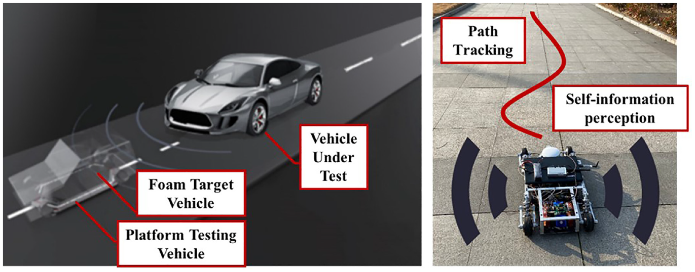
Application of testing platform vehicle.

The combined navigation system of Global Navigation Satellite System (GNSS) and Inertial Navigation System (INS) leverages the complementary strengths of both systems, providing more accurate, continuous, and reliable positioning information, thus representing the prevailing method in current navigation systems. Nonetheless, they still have drawbacks. When the testing platform vehicle enters an obstructed environment and the GNSS signal is lost, the navigation system has to rely solely on the INS. While the INS can provide accurate positioning information in the short term, long-term operation can lead to accumulate errors, eventually causing the positioning results to become invalid. ⁵

To resolve this issue, researchers have attempted to incorporate new sensors, utilizing supplementary observations to correct the long-term drift errors accumulated by the INS. Gao et al. ⁶ uses LIDAR to address positioning issues when GNSS signals are obstructed, but LIDAR is expensive, resource-intensive in computations, and performs poorly in open areas. In addition, researchers^7,8 tackle the problem of localization after GNSS signal loss by utilizing a Visual-Inertial Odometry (VIO) system, but VIO is susceptible to changes in ambient lighting and its own rotational movements, which can lead to a decrease in localization accuracy. Compared to LiDAR or camera, UWB offers higher accuracy, superior anti-interference capabilities, strong real-time performance, and relatively lower equipment and maintenance costs. Current researchers attempt to utilize UWB to address the positioning issues of testing vehicles when GNSS signals are weak or lost.^9,10 To achieve the desired positioning accuracy, the best fusion strategy for the GNSS, INS, and UWB sensors must be identified.

Many solutions for integrating GNSS, IMU, and UWB information are based on Kalman filters. ¹¹ However, they only rely on static fusion strategies to handle various environments, overlooking the issue of sensor failure caused by scenario transitions. This study introduces a GNSS/UWB/INS multi-sensor integrated navigation method, as shown in Figure 2, based on the Interacting Multiple Model (IMM), and proposes a novel Adaptive Transition Probability Matrix (ATPM). This matrix is updated using a Bayesian framework based on the measurement sequence and is used in cases where prior information is insufficient or inaccurate. Moreover, to resolve the computational and synchronization issues of multi-sensor information during online operation, the system adopts a frequency reduction method. In actual vehicle tests, we successfully addressed the smooth navigation mode switching issue during environmental changes, ensuring the stability and accuracy of the vehicle testing positioning system.

Figure 2.

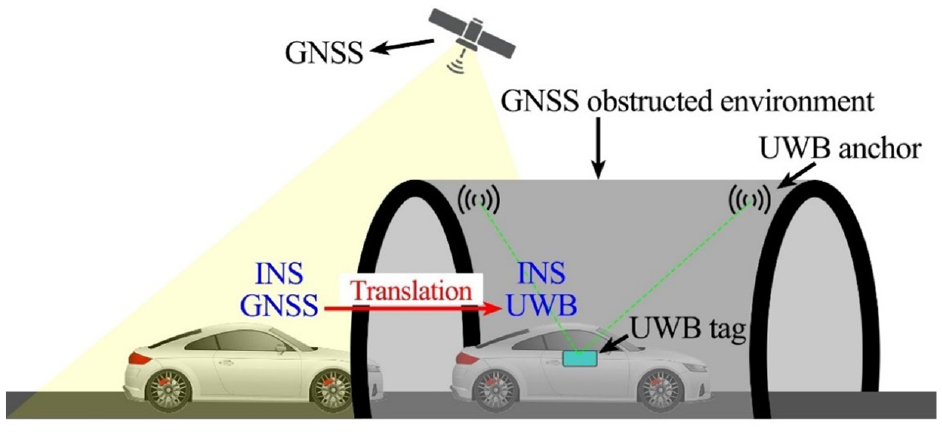
Switching of navigation method.

The main contributions of this study are as follows:

• This study introduces an advanced algorithm that integrates IMM and ESKF techniques. This algorithm effectively minimizes the impact of parameter singularities during computation and enhances the smoothness of transitions between models. Additionally, it addresses system positioning challenges caused by sensor failures due to scenario changes, ultimately improving the overall accuracy of the system’s positioning capabilities.

• This study proposes a novel Adaptive Transition Probability Matrix (ATPM) based on a Bayesian framework. By utilizing measurement sequences affected by environmental factors, it enhances current target state tracking and recalculates the transition probability matrix to adjust the model’s Markov jump probability. Compared to traditional transition probability matrices, this approach improves the system’s environmental adaptability.

• This study employs a frequency reduction method, reducing the computational load on the vehicle’s processor, increasing computational speed, and enhancing system real-time performance. Additionally, the robustness and positioning accuracy of the proposed algorithm were validated through experiments in both typical and challenging environments.

Related work

Multi-sensor fusion algorithm based on Kalman filter

Typically, the Kalman filter is used to solve linear problems, but to address the nonlinear issues in integrated positioning, researchers have proposed the Extended Kalman Filter (EKF). ¹² Vincenzo ¹³ integrated the UWB indoor positioning system into a GNSS/INS system based on EKF and geofencing algorithms to acquire synchronized data for further fusion analysis and seamless switching. To further address nonlinear problems, the Error State Kalman Filter (ESKF) was proposed. ESKF linearizes the system model around the equilibrium point to estimate the error state, providing better estimation results and is well-suited for integrated navigation systems with IMU sensors. Villien and Denis ¹⁴ used ESKF to integrate UWB distance measurements with a loosely coupled GNSS/INS system to improve positioning accuracy in challenging environments. Luo ⁹ enhanced the D-CEP algorithm to analyze UWB ranging variance, optimizing GNSS and UWB measurements using a variance-based nonlinear optimization method to obtain optimal observations, and then integrated these with IMU data through ESKF for optimal state estimation. However, these algorithms are still affected by faulty sensor data, leading researchers to propose the Federated Kalman Filter (FKF) to enhance the error adaptability and computational efficiency of positioning systems in dynamic environments. For instance, Zhang et al. ¹⁵ developed a MEMS-IMU/UWB/dual-antenna RTK-GNSS integrated navigation and positioning system based on an ARM microprocessor and FKF. Additionally, to improve the adaptability of the positioning system to the environment, filters incorporating error detection and information allocation have been proposed. Li et al. ¹⁶ proposed an improved Robust Kalman Filter for tightly coupled GNSS/UWB/IMU navigation, calculating the variance of the squared Mahalanobis distance within a moving window, introducing new anomaly detection factors, and reducing false positive rates in anomaly judgments. Liu et al. ¹⁷ used the Cubature Kalman Filter (CKF) and a threshold mechanism to achieve integrated positioning for outdoor GNSS/IMU and outdoor UWB/IMU. While these methods address the fusion of multi-sensor information to some extent, they overlook the issue of sensor failure caused by scenario switching.

Multi-sensor fusion algorithm for scene switching

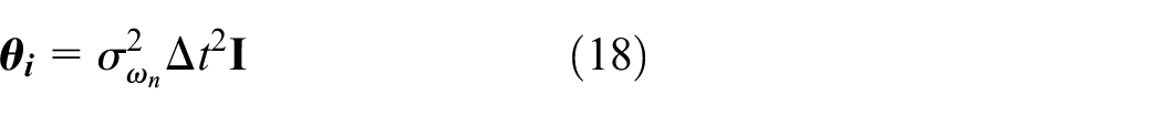
The Interacting Multiple Model (IMM) algorithm ¹⁸ has been proven to be applicable for target tracking and self-positioning of vehicles under different driving conditions, thus we can use the IMM algorithm to construct complex process models to solve sensor switching issues. For instance, Oliveira extensively discussed the use of principal component analysis and multiple model adaptive estimators to integrate feature-based positioning sensors for terrain-referenced navigation of underwater vehicles. Zhang et al. ¹⁹ proposed an Adaptive Interacting Multiple Model Unscented Kalman Filter (AIMM-UKF) to enhance the robustness of underwater robot navigation. Ndjeng ²⁰ applied IMM and EKF methods to solve outdoor vehicle positioning problems during abnormal maneuvers. Lu and Li ²¹ introduced the IMM algorithm as a means to develop a first-order GPB1-MHE (Generalized Pseudo Bayesian based Moving Horizon Estimation) method based on rolling time-domain estimation to predict the movement of surrounding vehicles, where the IMM sub-model serves MHE. Although most of these algorithms involve model switching, they still lack robustness and smoothness in sensor switching. Mu ²² proposed a resilient fusion method based on the Suboptimal Fusion Gain (SFG) algorithm, diagnosing sensor faults at the sensor layer through innovation mismatch assessment, and integrating GNSS/INS/odometer data at the decision layer using information sharing factors (ISF) derived from Fault Detection and Isolation (FDI). Meng and Hsu ²³ enhanced the IMM-based resilient Interactive Sensor Independent Update (ISIU) method by introducing trust priority of navigation sensors into information fusion, defining transition probability matrices in the form of Markov chains. Each observable sensor is integrated with the propagation system in an element filter with a sensor-independent update structure, achieving multi-sensor integration through interactive information fusion. These studies use EKF when processing sub-model data instead of ESKF. While addressing sub-model nonlinearity, they overlook the computational complexity of sub-model observations. Therefore, considering the need for switching among multiple modes, ²⁴ the algorithm must have the ability to judge and select models based on actual scenarios and demonstrate compatibility with ESKF. ²⁵ Our method integrates the advantages of the IMM and ESKF algorithms by utilizing an ATPM based on measurement data, which accelerates convergence speed, reduces the impact of faulty sensor data, and enhances both adaptability to changing environments and positioning accuracy.

Theoretical approach

At any given moment, the IMM algorithm conducts maneuver detection across multiple filtering models, adjusting the weights and model update probabilities of each filter to refine state estimation for targets exhibiting dynamic behavior. Each filter is configured with distinct state hypotheses, enabling the system to adaptively respond to variations in target behavior and environmental conditions. This adaptability enhances the matching of specific targets to achieve optimal fusion outcomes. A distinctive feature of the IMM algorithm is its use of transition probabilities to articulate the exchange of information during the transformation processes between various sub-models. These probabilities facilitate the algorithm’s flexible model transition based on the current state and motion dynamics of the target, ensuring a seamless transition process. The algorithm is capable of processing multiple information sources and updating the target state in real time. Through smooth transitions between different models, it mitigates the limitations inherent in using a single model for describing target motion and delivers precise predictions. Furthermore, the algorithm bolsters the robustness of target tracking in environments characterized by measurement noise and trajectory drift. As a result, even in scenarios where sensory data may be incomplete or erroneous, the algorithm maintains operational effectiveness, thus ensuring the reliability and accuracy of the data.^26,27,28

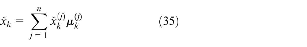
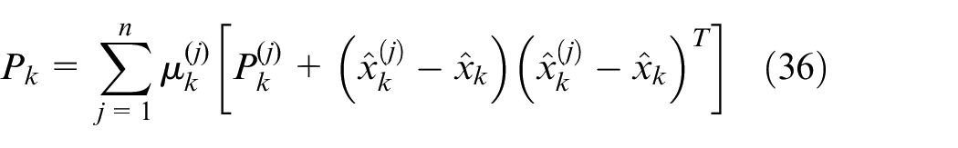
As shown in Figure 3, within the multi-sensor fusion model of this study, GNSS and UWB information are combined with IMU data, forming two models in the IMM algorithm. At each time step, each model independently and concurrently performs error filtering and prediction steps. When one model fails due to a change in the environment, it does not affect the operation of the other model. The initial conditions for the filter matching a specific model are obtained by mixing the state estimates from the previous time step with the transition probabilities between the two models. After updating the filters, the probability transition matrix is updated using the model matching likelihood function derived from the observation model adjustments. Finally, the corrected state estimates from all filters (model probabilities) are combined to produce the final state estimate.

Figure 3.

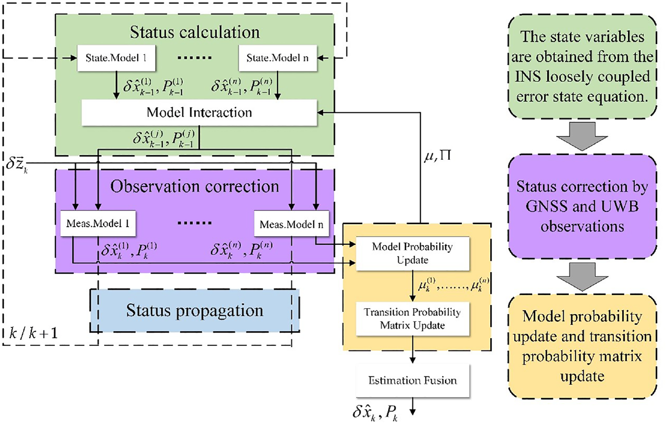
Schematic diagram of the proposed algorithm framework.

ESKF model

The process of IMM model is mainly as follows: Let the sub-models of the system at the $\mathit{k}$ moments be $M_k^{\left(1\right)},M_k^{\left(2\right)},\cdots ,M_k^{\left(n\right)}$ respectively. Taking the parallel filter $M_k^{\left(i\right)}$ as an example, according to the ESKF algorithm, then the present model $M_k^{\left(i\right)}$ can be expressed as follow:

$$\delta {\stackrel{·}{\hat{x}}}_k^{\left(i\right)}=F_k^{\left(i\right)}\delta {\hat{x}}_k^{\left(i\right)}+w_{k-1}^{\left(i\right)}$$

(1)

$$\delta {\overrightarrow{z}}_k^{\left(i\right)}=H_k^{\left(i\right)}\delta {\hat{x}}_{k-1}^{\left(i\right)}+{\gamma }_{k-1}^{\left(i\right)}$$

(2)

$$P_k^{\left(i\right)}=F_k^{\left(i\right)}{P}_{k-1}^{\left(i\right)}{F}_k^{\left(i\right)T}+{\mathit{Q}}_{k-1}^{\left(i\right)}$$

(3)

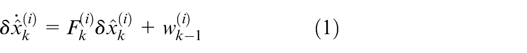
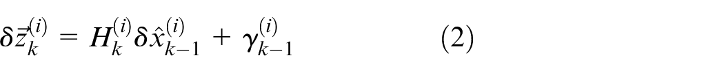
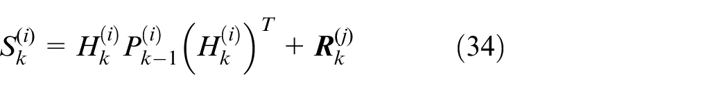
Where equations (1) and (2) represent the system equation and observation equation of the system, respectively, $\delta {\hat{x}}_k^{\left(i\right)}$ and $\delta {\overrightarrow{z}}_k^{\left(i\right)}$ denote the error state and the observation at moment $\mathit{k}-1$ . $F_k^{(i)}$ and $H_k^{\left(i\right)}$ denote the system transition matrix and the observation matrix. $w_{k-1}^{\left(i\right)}$ and ${\gamma }_{k-1}^{\left(i\right)}$ denote state noise and observation noise, which are mutually uncorrelated Gaussian white noise sequences with a mean of $\mathit{0}$ and can be expressed as follow:

$$E\left[w_{k-1}^{\left(i\right)}w\right]={\mathit{Q}}_{k-1}^{\left(i\right)}$$

(4)

$$E[{\gamma }_{k-1}^{\left(i\right)}{\gamma }_{k-1}^{\left(i\right)T}]={\mathit{R}}_{k-1}^{\left(i\right)}$$

(5)

${\mathit{Q}}_{k-1}^{\left(i\right)}$ and ${\mathit{R}}_{k-1}^{\left(i\right)}$ denote the system noise covariance matrix and the observation noise covariance matrix, respectively.

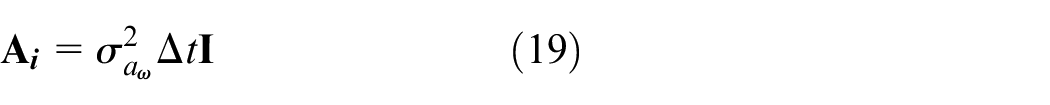
In the context of ESKF, the system state is a crucial concept that comprises a set of three fundamental state variables, namely the true state, nominal state, and error state. The true state is a compound of the nominal state and the error state, representing the actual state of the system. On the other hand, the nominal state is an abstract variable that represents the ideal state of the system, but cannot be estimated explicitly. During the fusion process, the estimated true state is used as the prediction to ensure the accuracy of the system. ²⁹ To facilitate the fusion of state estimates, this study has meticulously presented a list of error state that will be employed in the filtering process.

From the distribution of the true state of the system in Table 1, the error state equation of the system at the present $\mathit{k}$ moment can be derived, with the nominal state, IMU measurements and IMU noise on the right side of the equation. The notation $[{]}_{\times }$ represents the conversion of a vector into a skew-symmetric matrix.

$$\delta {\stackrel{·}{p}}_k=\delta v_k$$

(6)

$$\delta {\stackrel{·}{v}}_k=-R[a_{\mathrm{mk}}-{a_{\mathrm{bk}}]}_{\times }\delta {\theta }_k-R\delta a_{\mathrm{bk}}+\delta g-R{a}_n$$

(7)

$$\delta {\stackrel{·}{\theta }}_k=-[{\omega }_{\mathrm{mk}}-{{\omega }_{\mathrm{bk}}]}_{\times }\delta {\theta }_k-\delta {\omega }_{\mathrm{bk}}-{\omega }_n$$

(8)

$$\delta {\stackrel{·}{a}}_{\mathrm{bk}}=a_w$$

(9)

$$\delta {\stackrel{·}{\omega }}_{\mathrm{bk}}={\omega }_w$$

(10)

$$\delta \stackrel{·}{g}=0$$

(11)

Where $a_{\mathrm{mk}}$ and ${\omega }_{\mathrm{mk}}$ denote the acceleration and angular velocity obtained from the accelerometer and gyroscope measurements of the IMU. $a_w$ and ${\omega }_w$ denote accelerometer bias noise and gyroscope bias noise. $a_n$ and ${\omega }_n$ indicate accelerometer and gyroscope measurement noise. $R$ denotes the rotation matrix. While in the actual system, the system state quantities are non-continuous and in a discrete state. Therefore, we need to discretize the error state equation.

$$\delta p_{\mathit{k}+\mathrm{\Delta }\mathit{t}}=\delta p_{\mathit{k}}+\delta v_k\mathrm{\Delta }t$$

(12)

$$\begin{array}{c}\delta v_{\mathit{k}+\mathrm{\Delta }\mathit{t}}=\hfill \\ \delta v_k+(-R[a_{m\mathit{k}}-{a_{b\mathit{k}}]}_{\times }\delta \theta -R\delta a_{b\mathit{k}}+\delta g-R{a}_n)\mathrm{\Delta }t+{\mathit{V}}_i\hfill \end{array}$$

(13)

$$\delta {\theta }_{\mathit{k}+\nabla \mathit{t}}=R^T\{({\omega }_{m\mathit{k}}-{\omega }_{b\mathit{k}})\mathrm{\Delta }t\}\delta {\theta }_{\mathit{k}}-\delta {\omega }_{b\mathit{k}}\mathrm{\Delta }t+{\mathbf{\Theta }}_{\mathit{i}}$$

(14)

$$\delta a_{b\mathit{k}+\mathrm{\Delta }\mathit{t}}=\delta a_{b\mathit{k}}+{\mathbf{A}}_{\mathit{i}}$$

(15)

$$\delta {\omega }_{b\mathit{k}+\mathrm{\Delta }\mathit{t}}=\delta {\omega }_{b\mathit{k}}+{\mathbf{\Omega }}_{\mathit{i}}$$

(16)

Table 1.

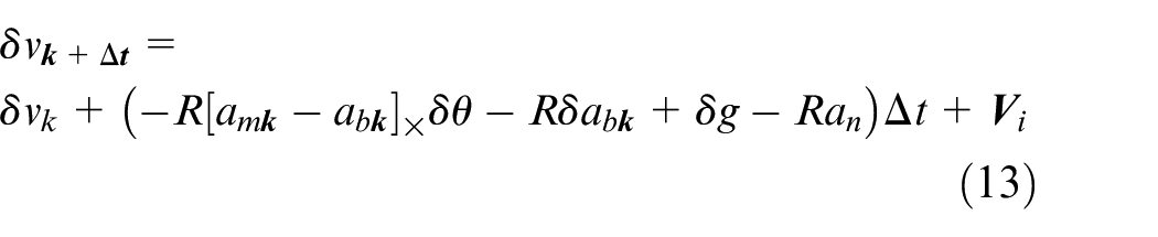
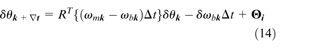
System state of the error state Kalman filter.

Magnitude	True	Nominal	Error	Composition
Full state	$x_k\left(t\right)$	$x_k$	$\delta x_k$	$x_k\left(t\right)=x_k+\delta x_k$
Position	$p_k\left(t\right)$	$p_k$	$\delta p_k$	$p_k\left(t\right)=p_k+\delta p_k$
Velocity	$v_k\left(t\right)$	$v_k$	$\delta v_k$	$v_k\left(t\right)=v_k+\delta v_k$
Euler Angle	${\theta }_k\left(t\right)$	${\theta }_k$	$\delta {\theta }_k$	${\theta }_k\left(t\right)={\theta }_k+\delta {\theta }_k$
Accelerometer bias	$a_{\mathrm{bk}}\left(t\right)$	$a_{\mathrm{bk}}$	$\delta a_{\mathrm{bk}}$	$a_{\mathrm{bk}}\left(t\right)=a_{\mathrm{bk}}+\delta a_{\mathrm{bk}}$
Gyrometer bias	${\omega }_{\mathrm{bk}}\left(t\right)$	${\omega }_{\mathrm{bk}}$	$\delta {\omega }_{\mathrm{bk}}$	${\omega }_{\mathrm{bk}}\left(t\right)={\omega }_{\mathrm{bk}}+\delta {\omega }_{\mathrm{bk}}$

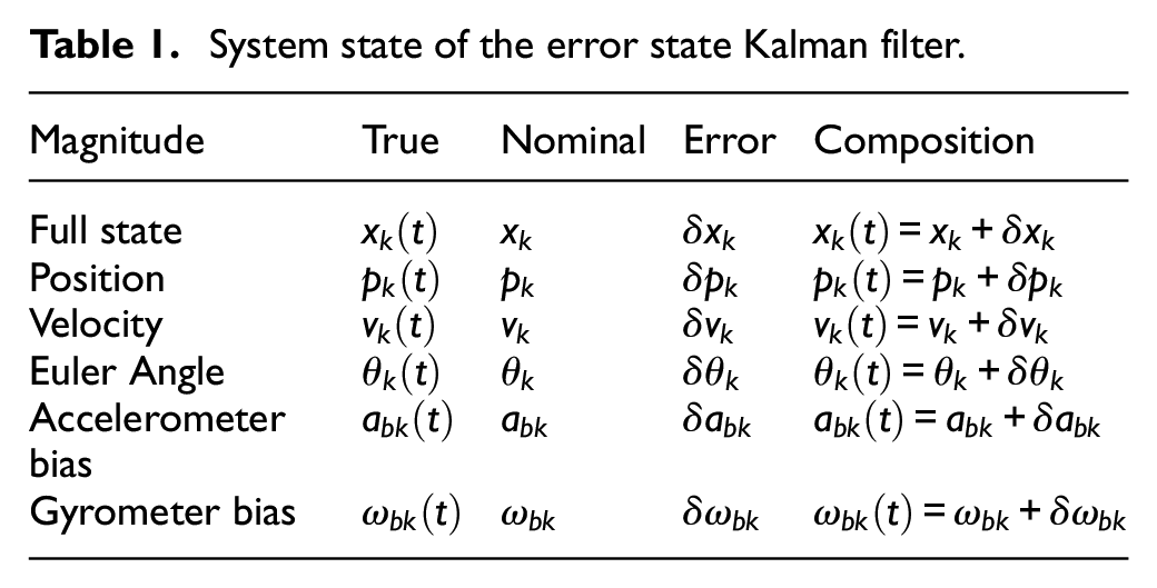
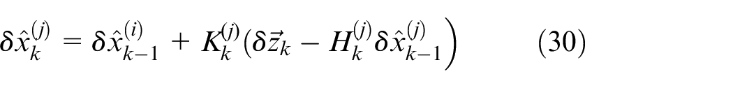
The symbol $I$ denotes the identity matrix. The random pulses ${\mathit{V}}_{i,}{\mathbf{\Theta }}_{\mathit{i}},{\mathbf{A}}_{\mathit{i},}{\mathbf{\Omega }}_{\mathit{i}}$ are applied to the velocity, angle, and bias, respectively. The values for these variables can be obtained by integrating the covariance of $a_n,{\omega }_n,a_{\omega },{\omega }_w$ over the time interval $\mathrm{\Delta }t$ as follows:

$${\mathit{V}}_{\mathit{i}}={\sigma }_{a_n}^2\mathrm{\Delta }{t}^2\mathbf{I}$$

(17)

$${\mathit{\theta }}_{\mathit{i}}={\sigma }_{{\omega }_n}^2\mathrm{\Delta }{t}^2\mathbf{I}$$

(18)

$${\mathbf{A}}_{\mathit{i}}={\sigma }_{a_{\omega }}^2\mathrm{\Delta }t\mathbf{I}$$

(19)

$${\mathbf{\Omega }}_{\mathit{i}}={\sigma }_{{\omega }_w}^2\mathrm{\Delta }t\mathbf{I}$$

(20)

Where ${\mathit{Q}}_{k-1}^i=\left[\begin{array}{cccc}{\mathit{V}}_i\hfill & 0\hfill & 0\hfill & 0\hfill \\ \multicolumn{1}{c}{0}& {\mathit{\theta }}_{\mathit{i}}\hfill & 0\hfill & 0\hfill \\ \multicolumn{1}{c}{0}& 0\hfill & {\mathbf{A}}_{\mathit{i}}\hfill & 0\hfill \\ \multicolumn{1}{c}{0}& 0\hfill & 0\hfill & {\mathbf{\Omega }}_{\mathit{i}}\hfill \end{array}\right]$ , and equation (1) can be rewritten as $\delta {\stackrel{·}{\hat{x}}}_k^{\left(i\right)}=F_k^{\left(i\right)}\delta {\hat{x}}_{k-1}^{\left(i\right)}$ . Here, $F_k^{\left(i\right)}$ denotes the Jacobian matrix of $f$ with respect to the error state, which can be expressed by the following equation:

$$\begin{array}{c}\multicolumn{1}{c}{F_k^{(i)}=\frac{\partial f}{\partial \delta {\hat{x}}_{k-1}^{\left(i\right)}}}\\ =\left[\begin{array}{cccccc}\mathbf{I}\hfill & \mathbf{I}\mathrm{\Delta }\mathrm{t}\hfill & 0\hfill & 0\hfill & 0\hfill & 0\hfill \\ \multicolumn{1}{c}{0}& \mathbf{I}\hfill & -R[a_{m\mathit{k}}-{a_{b\mathit{k}}]}_{\times }\mathrm{\Delta }\mathrm{t}\hfill & -R\mathrm{\Delta }\mathrm{t}\hfill & 0\hfill & \mathbf{I}\mathrm{\Delta }\mathrm{t}\hfill \\ \multicolumn{1}{c}{0}& 0\hfill & R^T\{({\omega }_{m\mathit{k}}-{\omega }_{b\mathit{k}})\mathrm{\Delta }t\}\hfill & 0\hfill & -\mathbf{I}\mathrm{\Delta }\mathrm{t}\hfill & 0\hfill \\ \multicolumn{1}{c}{0}& 0\hfill & 0\hfill & \mathbf{I}\hfill & 0\hfill & 0\hfill \\ \multicolumn{1}{c}{0}& 0\hfill & 0\hfill & 0\hfill & \mathbf{I}\hfill & 0\hfill \\ \multicolumn{1}{c}{0}& 0\hfill & 0\hfill & 0\hfill & 0\hfill & \mathbf{I}\hfill \end{array}\right]\hfill \end{array}$$

(21)

After completing the system equation of the sub-models $M_k^{\left(i\right)}$ , we assume that the real model of the system always exists in the set of sub-models, and let model $M_k^{\left(j\right)}$ be the real model of the system at moment $\mathit{k}$ then the interaction process can be expressed as:

$$\delta {\hat{x}}_{k-1}^{\left(j\right)}=\sum _{i=1}^n\delta {\hat{x}}_{k-1}^{\left(i\right)}{\mu }_{k-1|k-1}^{\left(i\right)|(j)}$$

(22)

$$\begin{array}{c}{P}_{k-1}^{(j)}=\hfill \\ \sum _{i=1}^n[P_{k-1}^{(j)}+(\delta {\hat{x}}_{k-1}^{\left(i\right)}-\delta {\hat{x}}_{k-1}^{\left(j\right)})(\delta {\hat{x}}_{k-1}^{\left(i\right)}-{\delta {\hat{x}}_{k-1}^{\left(j\right)})}^T]·{\mu }_{k-1|k-1}^{\left(i\right)|(j)}\hfill \end{array}$$

(23)

$$\overline{c_J}=\sum _{i=1}^n{p}_{\mathrm{ij}}{\mu }_{k-1}^{(i)}$$

(24)

In the given equation, the variable $\delta {\hat{x}}_{k-1}^{\left(j\right)}$ refers to the state at time $\mathit{k}-1$ , which is a combination of the error state $\delta {\hat{x}}_{k-1}^{\left(i\right)}$ from two systems mixed in a certain proportion. The term $P_{k-1}^{(j)}$ denotes the covariance matrix obtained by mixing the covariance matrix $P_{k-1}^{(i)}$ from various models. The input interaction facilitates the interaction between the two sets of models from the previous time step, aiding in the acquisition of the mixed initial state of the GNSS/INS and UWB/INS filters. The term ${\mu }_{k-1|k-1}^{\left(i\right)|(j)}$ represents the comprehensive transition probability from model $i$ to model $j$ , determined by the model’s prediction normalization constant $\overline{c_J}$ and the previous time step model probability ${\mu }_{k-1}^{(i)}$ (i.e. the probability of accurately describing the target state as ${\mu }_{k-1}^{(i)}=P(M_{k-1}^{(i)}|\delta {\overrightarrow{z}}_{k-1}^{\left(i\right)})$ and the model probability transition probability $p_{\mathrm{ij}}$ ). This probability can be computed as follow:

$${\mu }_{k-1|k-1}^{\left(i\right)|(j)}=\frac{\sum _{i=1}^n{p}_{\mathrm{ij}}{\mu }_{k-1}^{(i)}}{\overline{c_j}}$$

(25)

The variable $p_{\mathrm{ij}}$ denotes the transition probability of a stochastic process between models $i$ and j according to the Markov principle. More specifically, given a set of random models $\mathit{M}=\{M_k^{(n)}:n>0\}$ at time $\mathit{k}$ , $p_{\mathrm{ij}}$ signifies the likelihood of model $M_{k-1}^{(i)}$ transitioning to model $M_k^{(j)}$ from time $\mathit{k}-1$ to time $\mathit{k}$ . Furthermore, the conditional probability of the random model satisfies the following relation:

$$P(M_k^{\left(n\right)}|M_k^{(n-1)},M_k^{(n-2)},\cdots ,M_k^{\left(1\right)})=P(M_k^{\left(n\right)}|M_k^{(n-1)})$$

(26)

In the context of a multi-model system, as shown in Figure 4, various sensors are located at different interfaces, which imparts them with a degree of independence from one another. Specifically, one sub-model $M_k^{(i)}$ can only provide observations that pertain to its specific interface, without influencing the observations provided by sensors associated with other models. As a result, the different models within the system remain relatively independent of each other. The probability of stochastic transitions between models is also independent. ²³

Figure 4.

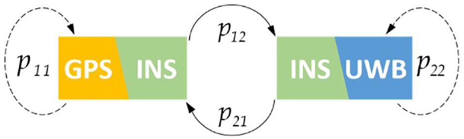
Schematic diagram of model jump.

Judgment of model

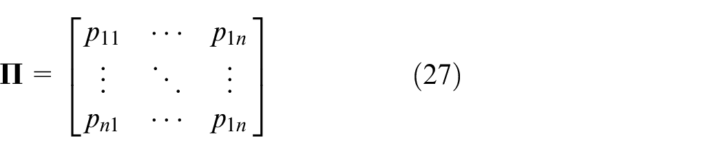
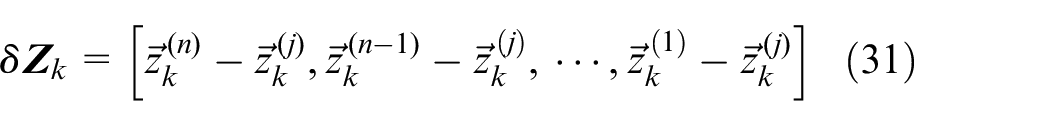
The following equation provides a representation of the TPM for the filtering method used in this study:

$$\mathbf{\Pi }=\left[\begin{array}{ccc}{p}_{11}\hfill & \cdots \hfill & p_{1n}\hfill \\ \multicolumn{1}{c}{⋮}& \ddots \hfill & ⋮\hfill \\ \multicolumn{1}{c}{p_{n1}}& \cdots \hfill & p_{1n}\hfill \end{array}\right]$$

(27)

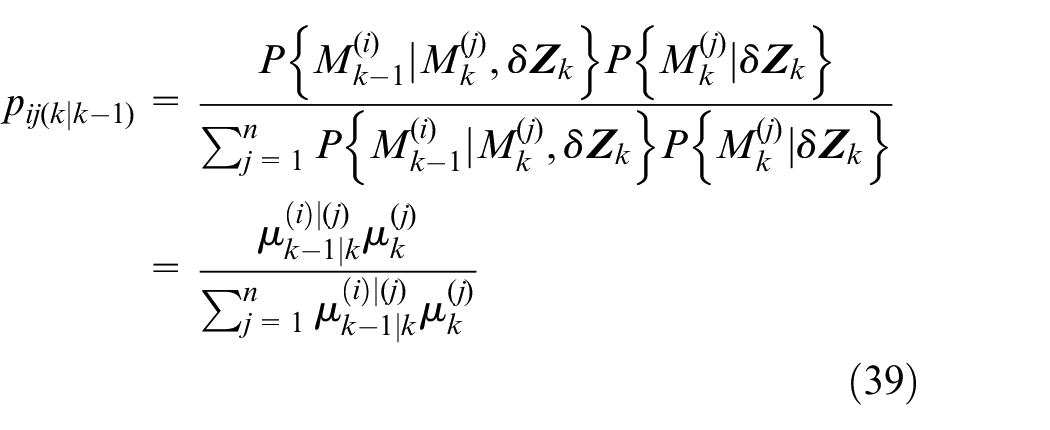
When the previous moment system mixture values $\delta {\hat{x}}_{k-1}^{\left(i\right)}$ , $P_{(k-1)}^{\left(j\right)}$ from equations (22) and (23) are obtained, this value is substituted into the filter update phase, that is, the system state estimates corresponding to the individual model filter outputs at moment k and the covariance estimates:

$$K_k^{(j)}=P_{k-1}^{\left(j\right)}(H_k^{\left(i\right)}{)}^T(H_k^{\left(i\right)}{P_{(k-1)}^{\left(j\right)}{(H_k^{\left(i\right)})}^T+R_k^{(j)})}^{-1}$$

(28)

$$P_k^{\left(j\right)}=P_{k-1}^{\left(j\right)}-K_k^{(j)}{H}_k^{\left(i\right)}{P}_{k-1}^{\left(j\right)}$$

(29)

$$\delta {\hat{x}}_k^{\left(j\right)}=\delta {\hat{x}}_{k-1}^{\left(i\right)}+K_k^{(j)}(\delta {\overrightarrow{z}}_k-H_k^{\left(j\right)}\delta {\hat{x}}_{k-1}^{\left(j\right)})$$

(30)

In the above equation, $K_k^{(j)}$ denotes the Kalman gain of model j at time $\mathit{k}$ . The Kalman filtering values $P_k^{\left(j\right)}$ and $\delta {\hat{x}}_k^{\left(j\right)}$ that accurately describe the system at time $\mathit{k}$ can be obtained using the equation. After the observation correction stage, real-time model updating is achieved through the likelihood function. By computing the similarity between the model and the present target state, weights are assigned to determine the most suitable localization model, thus facilitating the update of the posterior probability ${\mu }_k^{(i)}$ of the model. For different model $i$ , the difference between the multi-sensor observation $\delta {\overrightarrow{z}}_k^{(i)}$ and the observation ${\overrightarrow{z}}_k^{(j)}$ that accurately matches the present model can be computed as follow:

$$\delta {\mathit{Z}}_k=[{\overrightarrow{z}}_k^{(n)}-{\overrightarrow{z}}_k^{(j)},{\overrightarrow{z}}_k^{(n-1)}-{\overrightarrow{z}}_k^{\left(j\right)},\cdots ,{\overrightarrow{z}}_k^{\left(1\right)}-{\overrightarrow{z}}_k^{(j)}]$$

(31)

In the processing of ESKF, the model innovation is usually calculated as follows:

$$\delta {\tilde{z}}_k^{(i)}=\delta {\overrightarrow{z}}_k^{(i)}-H_k^{\left(i\right)}\delta {\hat{x}}_k^{\left(i\right)}$$

(32)

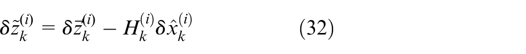
Then the maximum likelihood function of the observation error at moment $\mathit{k}$ for different model $i$ is as follow:

$${\mathrm{\Lambda }}_k^{(i)}=\frac{1}{\sqrt{2\pi ·\det \left(S_k^{(i)}\right)}}\exp [-\frac{1}{2}{(\delta {\tilde{z}}_k^{\left(i\right)})}^T{\left(S_k^{(i)}\right)}^{-1}\delta {\tilde{z}}_k^{\left(i\right)}]$$

(33)

$$S_k^{(i)}=H_k^{\left(i\right)}{P}_{k-1}^{\left(i\right)}{\left(H_k^{\left(i\right)}\right)}^T+{\mathit{R}}_k^{(j)}$$

(34)

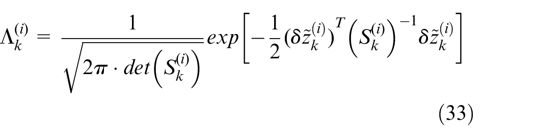
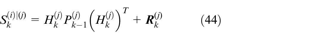
In metrological terminology, $S_k^{(i)}$ denotes the innovation covariance matrix of the model $i$ , which is a $N\times N$ matrix. The det operation represents the determinant of the matrix, and the exp operation represents the natural logarithm. Once the maximum likelihood function update is completed, it is necessary to update the probability or credibility of each model ${\mu }_k^{(i)}$ in time $\mathit{k}$ .

$${\mu }_k^{(i)}=\frac{{\mathrm{\Lambda }}_k^{(i)}\left[{\sum }_{i=1}^n{p}_{\mathrm{ij}}{\mu }_{k-1}^{(i)}\right]}{{\sum }_{i=1}^n{\mathrm{\Lambda }}_k^{(j)}\left[{\sum }_{i=1}^n{p}_{\mathrm{ij}}{\mu }_{k-1}^{(i)}\right]}$$

(35)

The obtained state estimates and covariances $P_k^{\left(j\right)}$ and $\delta {\hat{x}}_k^{\left(j\right)}$ of all models from equations (29) and (30) are combined with appropriate weights. The weight assigned to each model corresponds to the probability of its match with the present system model calculated using the above equation. The resulting weighted sum yields the final state estimate and its covariance at the current time.

$${\hat{x}}_k=\sum _{j=1}^n{\hat{x}}_k^{\left(j\right)}{\mu }_k^{(j)}$$

(35)

$$P_k=\sum _{j=1}^n{\mu }_k^{(j)}[P_k^{(j)}+({\hat{x}}_k^{\left(j\right)}-{\hat{x}}_k){({\hat{x}}_k^{\left(j\right)}-{\hat{x}}_k)}^T]$$

(36)

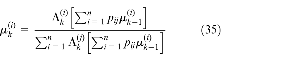
Adaptive transition probability matrix (ATPM)

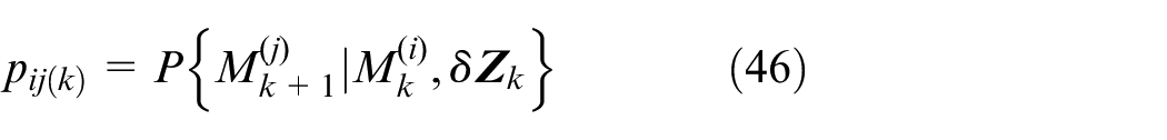
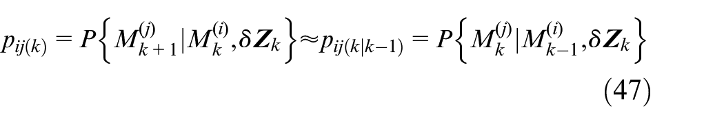
For the above derivation of the computational procedure of IMM it can be seen that the IMM algorithm uses a fixed TPM based on a priori information. The transfer probability is defined by the following equation:

$$p_{\mathrm{ij}(k-1)}=P\{M_k^{(j)}|M_{k-1}^{(j)},\delta {\mathit{Z}}_{k-1}\}$$

(37)

In the equation, $\delta {\mathit{Z}}_{k-1}$ represents a collection of observations as indicated by equation (31). In the event of insufficient or inaccurate prior information leading to a mismatch between the initial value of the TPM and the actual system model, ³⁰ the TPM remains static throughout the process, which impedes real-time tracking of the target state and reduces the tracking accuracy of the system. Consequently, accurate positioning mode switching becomes challenging, hence the need for adaptive TPM updates. After obtaining the observation value $\delta {\mathit{Z}}_k$ at time $\mathit{k}$ , $p_{\mathrm{ij}(k-1)}$ is recursively propagated to $p_{\mathrm{ij}(k)}$ . This study defines $p_{\mathrm{ij}(k|k-1)}$ as the posterior estimate of the TPM based on the observation value $\delta {\mathit{Z}}_k$ at time $\mathit{k}-1$ , as shown in the following equation:

$$p_{\mathrm{ij}(k|k-1)}=P\{M_k^{(j)}|M_{k-1}^{(j)},\delta {\mathit{Z}}_k\}$$

(38)

$p_{\mathrm{ij}(k|k-1)}$ can be considered as the posterior estimate of the model transition probability based on time $\mathit{k}-1$ . According to Bayes’ theorem, $p_{\mathrm{ij}(k|k-1)}$ can be further expressed as:

$$\begin{array}{c}\multicolumn{1}{c}{p_{\mathrm{ij}(k|k-1)}=\frac{P\{M_{k-1}^{(i)}|M_k^{(j)},\delta {\mathit{Z}}_k\}P\{M_k^{(j)}|\delta {\mathit{Z}}_k\}}{{\sum }_{j=1}^{n}P\{M_{k-1}^{(i)}|M_k^{(j)},\delta {\mathit{Z}}_k\}P\{M_k^{(j)}|\delta {\mathit{Z}}_k\}}}\\ =\frac{{\mu }_{k-1|k}^{\left(i\right)|(j)}{\mu }_k^{(j)}}{{\sum }_{j=1}^n{\mu }_{k-1|k}^{\left(i\right)|(j)}{\mu }_k^{(j)}}\hfill \end{array}$$

(39)

Where ${\mu }_{k-1|k}^{\left(i\right)|(j)}$ is defined as when the observations $\delta {\mathit{Z}}_k$ have been obtained and the time $\mathit{k}$ model $M_k^{(j)}$ is valid. So, probability of model $M_{k-1}^{(i)}$ at $\mathit{k}-1$ is as follows:

$${\mu }_{k-1|k}^{\left(i\right)|(j)}=P\{M_{k-1}^{(j)}|M_{k-1}^{(j)},\delta {\mathit{Z}}_{k-1}\}$$

(40)

The meaning of the model probability ${\mu }_{k-1|k}^{\left(i\right)|(j)}$ at the previous moment is described above. Then, according to the conditional probability formula and the full probability formula, ${\mu }_{k-1|k}^{\left(i\right)|(j)}$ can be further represented as:

$$\begin{array}{c}\multicolumn{1}{c}{{\mu }_{k-1|k}^{\left(i\right)|(j)}=P\{M_{k-1}^{(j)}|\delta {\overrightarrow{z}}_k^{(j)},M_k^{(j)},\delta {\mathit{Z}}_{k-1}\}}\\ =\frac{{\mathrm{\Lambda }}_k^{\left(i\right)|(j)}{p}_{\mathrm{ij}(k-1)}{\mu }_{k-1}^{(i)}}{{\sum }_{i=1}^n\left[{\mathrm{\Lambda }}_k^{\left(i\right)|(j)}{p}_{\mathrm{ij}(k-1)}{\mu }_{k-1}^{(i)}\right]}\hfill \end{array}$$

(41)

Where ${\mathrm{\Lambda }}_k^{\left(i\right)|(j)}$ is a likelihood function. From the definition of the likelihood function, the transition likelihood from $M_{k-1}^{(i)}$ to $M_k^{(j)}$ can be expressed as follows:

$$\begin{array}{c}{\mathrm{\Lambda }}_k^{\left(i\right)|(j)}=\hfill \\ \frac{1}{\sqrt{2\pi ·\det \left(S_k^{\left(i\right)|(j)}\right)}}\exp [-\frac{1}{2}{(\delta {\tilde{z}}_k^{\left(i\right)|(j)})}^T{\left(S_k^{\left(i\right)|(j)}\right)}^{-1}\delta {\tilde{z}}_k^{\left(i\right)|(j)}]\hfill \end{array}$$

(42)

$$\delta {\tilde{z}}_k^{\left(i\right)|(j)}=\delta {\overrightarrow{z}}_k^{(i)}-H_k^{(j)}\delta {\hat{x}}_k^{\left(j\right)}$$

(43)

$$S_k^{\left(i\right)|(j)}=H_k^{\left(j\right)}{P}_{k-1}^{\left(j\right)}{\left(H_k^{\left(j\right)}\right)}^T+{\mathit{R}}_k^{(j)}$$

(44)

Where $\delta {\tilde{z}}_k^{\left(i\right)|(j)}$ represents the new information process of the observation $\delta {\overrightarrow{z}}_k^{(i)}$ and the model $M_k^{(j)}$ ; $S_k^{\left(i\right)|(j)}$ is its corresponding covariance matrix. So far, the final equation for $p_{\mathrm{ij}(k|k-1)}$ is:

$$p_{\mathrm{ij}(k|k-1)}=\frac{\frac{{\mathrm{\Lambda }}_k^{\left(i\right)|(j)}{p}_{\mathrm{ij}(k-1)}{\mu }_{k-1}^{\left(i\right)}{\mu }_k^{\left(j\right)}}{{\sum }_{i=1}^n\left[{\mathrm{\Lambda }}_k^{\left(i\right)|(j)}{p}_{\mathrm{ij}(k-1)}{\mu }_k^{\left(i\right)}\right]}}{{\sum }_{j=1}^n\left[\frac{{\mathrm{\Lambda }}_k^{\left(i\right)|(j)}{p}_{\mathrm{ij}(k-1)}{\mu }_{k-1}^{\left(i\right)}{\mu }_k^{\left(j\right)}}{\sum _{i=1}^n{\mathrm{\Lambda }}_k^{\left(i\right)|(j)}{p}_{\mathrm{ij}(k-1)}{\mu }_{k-1}^{\left(i\right)}}\right]}$$

(45)

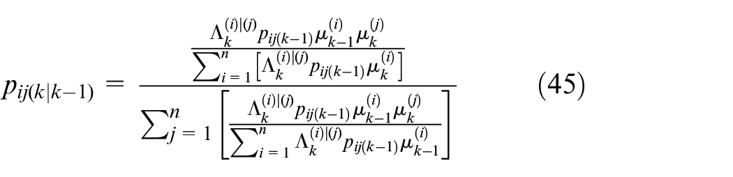
After getting $p_{\mathrm{ij}(k|k-1)}$ , in order to get $p_{\mathrm{ij}(k)}$ , the relationship between $p_{\mathrm{ij}(k|k-1)}$ and $p_{\mathrm{ij}(k)}$ needs to be established. For $p_{\mathrm{ij}(k)}$ :

$$p_{\mathrm{ij}\left(k\right)}=P\{M_{k+1}^{(j)}|M_k^{(i)},\delta {\mathit{Z}}_k\}$$

(46)

For a model at the present $\mathit{k}$ , the model transfer probability of $M_{k+1}^{(j)}$ is difficult to obtain, so it is considered that for $\delta {\mathit{Z}}_k$ of the same observation series, the model transfer probability from $\mathit{k}-1$ to $\mathit{k}$ is approximately equal, as shown below:

$$p_{\mathrm{ij}\left(k\right)}=P\{M_{k+1}^{(j)}|M_k^{(i)},\delta {\mathit{Z}}_k\}\approx p_{\mathrm{ij}(k|k-1)}=P\{M_k^{(j)}|M_{k-1}^{(i)},\delta {\mathit{Z}}_k\}$$

(47)

So, we get the final expression for $p_{\mathrm{ij}\left(k\right)}$ :

$$p_{\mathrm{ij}\left(k\right)}=\frac{\frac{{\mathrm{\Lambda }}_k^{\left(i\right)|(j)}{p}_{\mathrm{ij}(k-1)}{\mu }_{k-1}^{\left(i\right)}{\mu }_k^{\left(j\right)}}{{\sum }_{i=1}^n\left[{\mathrm{\Lambda }}_k^{\left(i\right)|(j)}{p}_{\mathrm{ij}(k-1)}{\mu }_{k-1}^{\left(i\right)}\right]}}{{\sum }_{j=1}^n\left[\frac{{\mathrm{\Lambda }}_k^{\left(i\right)|(j)}{p}_{\mathrm{ij}(k-1)}{\mu }_{k-1}^{\left(i\right)}{\mu }_k^{\left(j\right)}}{{\sum }_{i=1}^n{\mathrm{\Lambda }}_k^{\left(i\right)|(j)}{p}_{\mathrm{ij}(k-1)}{\mu }_{k-1}^{\left(i\right)}}\right]}$$

(48)

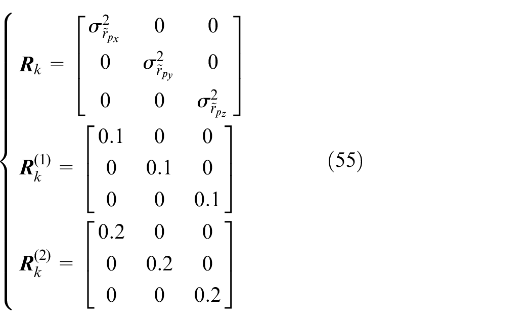
By utilizing this method of adaptive model transition probability correction based on measurement data, the impact of matching models is magnified while that of non-matching models is dampened. The transition process takes advantage of the information from the matching models more, and minimizes the influence of non-matching models, ultimately resulting in an accelerated convergence rate.

The corrected transition probability continues to satisfy the two essential properties of transition probability, which are:

$$0<p_{\mathrm{ij}}<1,i,j=1,2,\cdots ,n$$

(49)

$$\sum _p^n{p}_{\mathrm{ij}}=1$$

(50)

Sensor frequency standardization

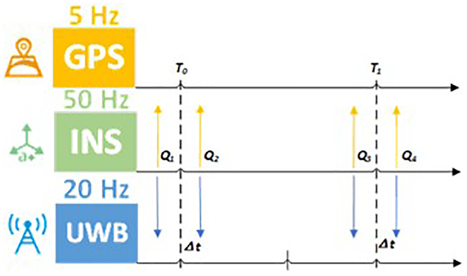
In experiment, the lack of uniformity in signal frequencies from multiple sensors can pose significant challenges. Non-equal sampling frequencies of sensor signals can result in asynchrony of signal timestamps, which can subsequently impact signal fusion outcomes. To address this issue, various approaches can be adopted, including:

1)     Standardizing the frequency of high-frequency signals to low-frequency signals;

2)     Interpolating the timestamps of high-frequency signals and integrating them into low-frequency signals. ³¹

Such strategies can help align signal timestamps and facilitate signal fusion. In this study, the computational environment comprised of Ubuntu 20.04 system with an i7-7700k processor and Python 3.6 as the algorithmic language environment. The system computed the computing time per step in the typical experimental environment of this study, using both linear interpolation and no interpolation methods, as shown in Table 2.

Table 2.

Comparison of computation time between interpolation and frequency reduction methods in experiments under typical environments.

Datasets	Methods	ESKF	IMM	ATPM-IMM
Case 1	Interpolation	0.047 ms/step	0.254 ms/step	0.261 ms/step
	Frequency reduction	0.029 ms/step	0.141 ms/step	0.145 ms/step
Case 2	Interpolation	0.049 ms/step	0.317 ms/step	0.333 ms/step
	Frequency reduction	0.028 ms/step	0.195 ms/step	0.207 ms/step

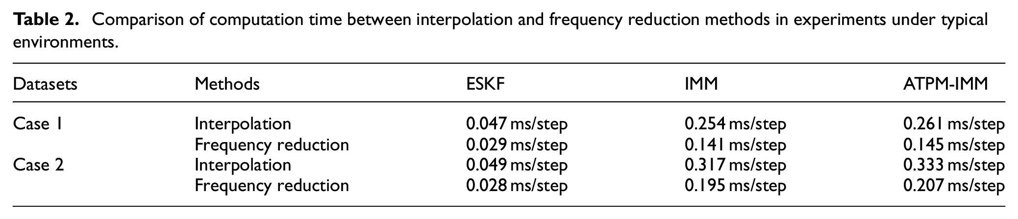
As shown in Figure 5, this study employs signal frequency reduction techniques to decrease the sampling rates of high-frequency signals, aligning them with those of other sensors to reduce the volume of signal data and enhance the efficiency of signal processing. By processing GNSS, IMU, and UWB data at a lower frequency, as demonstrated in Table 2, the processing speed of the hardware is improved. Consequently, the positioning algorithm developed in this research, which integrates complementary information, can meet the real-time requirements in dynamic environments to some extent. Within the ROS framework, multithreading priority management is effectively utilized to downsample data from various sensors. The downsampling process involves selecting a specific number of data points based on each sensor’s original frequency. For example, for an IMU with an original frequency of 50 Hz, downsampling to 5 Hz is achieved by selecting one out of every ten data points. Similarly, for UWB with an original frequency of 20 Hz, one out of every four data points is chosen to reduce the frequency to 5 Hz. Finally, by processing the data from GNSS, IMU, and UWB within a unified time window, this research achieves soft synchronization and timestamp alignment, thereby effectively facilitating signal fusion.

Figure 5.

Interpolation method for signals from multiple sensors.

Experiment and discussion

Experiment preparation

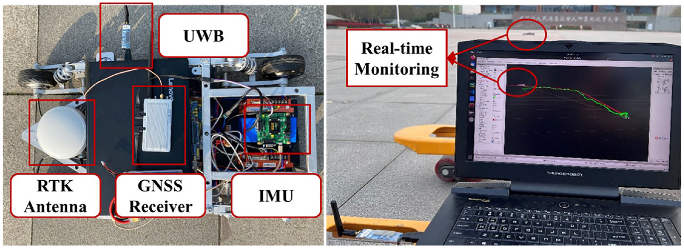
Given the cost and size limitations of the testing platform vehicle, this study integrates low-cost and compact sensor accessories onto the existing structure and control system of the vehicle. The aim is to reduce the cost of the testing platform vehicle and enhance its compatibility with the model vehicle. The GNSS is utilized to retrieve GPGGA data that includes the experiment’s latitude and longitude information for the testing platform vehicle. The IMU is used to collect real-time data on the testing platform vehicle’s three-axis acceleration and three-axis angular velocity. The UWB is employed to measure the real-time distance between the anchor and the tag. The proposed algorithm is then used to solve the present position information of the testing platform vehicle, as illustrated in Figure 6. The research team employed two master computers, both equipped with Linux and ROS, for data collection and processing. One of the computers was mounted on the testing platform vehicle, serving as a calculation terminal, while the other was designated as a data monitoring terminal. The two master computers exchanged data through ROS topic communication within the same local area network. Real-time positioning data of the testing platform vehicle were monitored and displayed using Rviz. The GNSS and UWB sensors were connected to the testing platform vehicle’s calculation terminal using a serial port connection.

Figure 6.

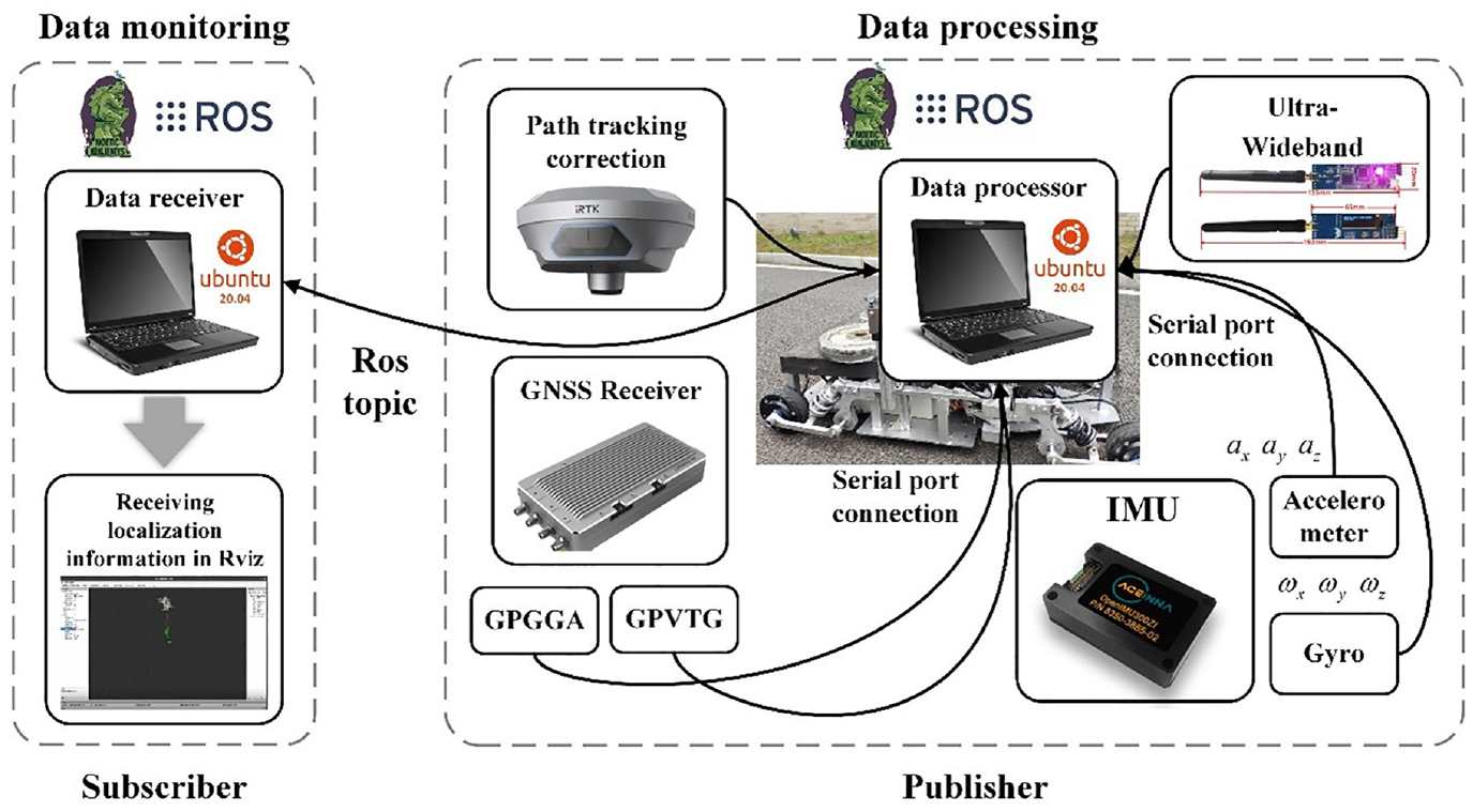
Data protocols used by sensors.

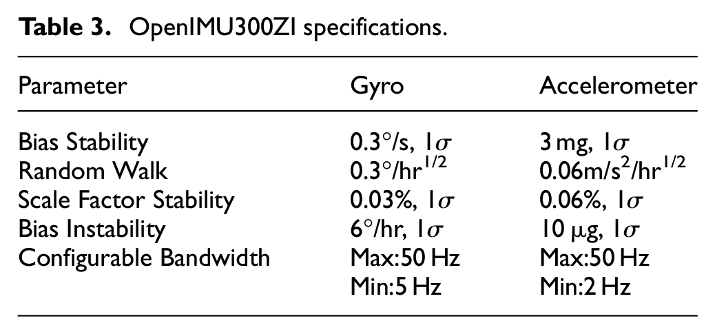
The low-cost IMU used in this study, such as the OpenIMU300ZI, consists of a three-axis gyroscope, a three-axis accelerometer, and a magnetometer. The specifications are listed in Table 3. The IMU sensor is powered by a 168 Hz ARM M4 CPU and a floating-point unit, and supports Windows and Ubuntu systems.

Table 3.

OpenIMU300ZI specifications.

Parameter	Gyro	Accelerometer
Bias Stability	0.3°/s, 1σ	3 mg, 1σ
Random Walk	0.3°/hr1/2	0.06m/s2/hr1/2
Scale Factor Stability	0.03%, 1σ	0.06%, 1σ
Bias Instability	6°/hr, 1σ	10 μg, 1σ
Configurable Bandwidth	Max:50 Hz Min:5 Hz	Max:50 Hz Min:2 Hz

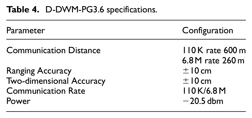
The experimental setup utilized the D-DWM-PG 3.6 UWB kit, which was sourced from Guangzhou Lianwang Technology. The kit is capable of measuring distances with an accuracy of ±10cm, within a range of 600 m, using the Time-Weighted Time of Flight (TW-TOF) principle for location determination. The UWB measurement parameters are detailed in Table 4, and the system is notable for its low cost and low power consumption.

Table 4.

D-DWM-PG3.6 specifications.

Parameter	Configuration
Communication Distance	110 K rate 600 m 6.8 M rate 260 m
Ranging Accuracy	±10 cm
Two-dimensional Accuracy	±10 cm
Communication Rate	110 K/6.8 M
Power	−20.5 dbm

Experiment settings

To validate and evaluate the positional accuracy of the self-developed testing platform vehicle, an onboard computer is incorporated, which is connected to the UWB, GNSS, and IMU modules via a serial port. The UWB module comprises three anchors, which are securely positioned vertically in the testing field to ensure they are situated in the same plane. The diagram of experiment configuration is depicted in Figure 7. Some filter parameters in the experiments are as follows ¹⁹ :

$$\{\begin{array}{c}{\mathit{Q}}_k=[{\sigma }_{{\tilde{a}}_{n_x}}^2,{\sigma }_{{\tilde{a}}_{n_y}}^2,{\sigma }_{{\tilde{a}}_{n_y}}^2,{\sigma }_{{\tilde{\omega }}_{n_x}}^2,{\sigma }_{{\tilde{\omega }}_{n_y}}^2,{\sigma }_{{\tilde{\omega }}_{n_z}}^2,{\sigma }_{{\tilde{a}}_{w_x}}^2,{\sigma }_{{\tilde{a}}_{w_y}}^2,{\sigma }_{{\tilde{a}}_{w_z}}^2,{\sigma }_{{\tilde{\omega }}_{w_x}}^2,{\sigma }_{{\tilde{\omega }}_{w_y}}^2,{\sigma }_{{\tilde{\omega }}_{w_z}}^2]·\hfill \\ \mathrm{diag}({\mathbf{I}}_{12\times 1})\hfill \\ {\mathit{Q}}_k=\mathrm{diag}(0.1·{\mathbf{I}}_{12\times 1})\hfill \end{array}$$

(51)

$$\delta {\overrightarrow{z}}_k=[\delta {\overrightarrow{z}}_{k_{p_x}},\delta {\overrightarrow{z}}_{k_{p_y}},\delta {\overrightarrow{z}}_{k_{p_z}}]$$

(52)

$$\delta {\mathit{Z}}_k=[\delta {\overrightarrow{z}}_{k(\mathrm{GNSS}/\mathrm{INS})},\delta {\overrightarrow{z}}_{k(\mathrm{UWB}/\mathrm{INS})}]$$

(53)

$$\delta {\hat{x}}_k=\left[\delta P_x\delta P_y\delta P_z\delta V_x\delta V_y\delta V_z\delta {\varphi }_x\delta {\varphi }_y\delta {\varphi }_z{\epsilon }_x{\epsilon }_y{\epsilon }_z{\nabla }_x{\nabla }_y{\nabla }_z\right]$$

(54)

$$\{\begin{array}{c}{\mathit{R}}_k=\left[\begin{array}{ccc}{\sigma }_{{\tilde{r}}_{p_x}}^2\hfill & 0\hfill & 0\hfill \\ \multicolumn{1}{c}{0}& {\sigma }_{{\tilde{r}}_{p_y}}^2\hfill & 0\hfill \\ \multicolumn{1}{c}{0}& 0\hfill & {\sigma }_{{\tilde{r}}_{p_z}}^2\hfill \end{array}\right]\hfill \\ {\mathit{R}}_k^{(1)}=\left[\begin{array}{ccc}0.1\hfill & 0\hfill & 0\hfill \\ \multicolumn{1}{c}{0}& 0.1\hfill & 0\hfill \\ \multicolumn{1}{c}{0}& 0\hfill & 0.1\hfill \end{array}\right]\hfill \\ {\mathit{R}}_k^{(2)}=\left[\begin{array}{ccc}0.2\hfill & 0\hfill & 0\hfill \\ \multicolumn{1}{c}{0}& 0.2\hfill & 0\hfill \\ \multicolumn{1}{c}{0}& 0\hfill & 0.2\hfill \end{array}\right]\hfill \end{array}$$

(55)

Figure 7.

Experiment configuration.

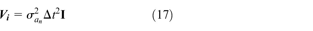
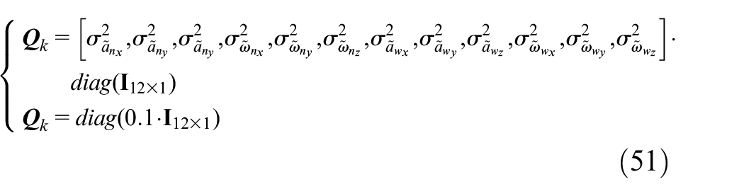
Furthermore, UWB only participates in the calculation of data relative to the carrier coordinates and does not have velocity and angle information, ³² so the observation needs adjustment. Consequently, the measurement noise matrix of the system also requires corresponding adjustments. In reality, the covariance of measurement noise ${\mathit{R}}_k$ is time-varying, and a fixed ${\mathit{R}}_k$ will, to some extent, decrease the navigation accuracy of the testing platform vehicle.

In this study, the initial transition matrix was established as shown in equation (56). This technique can result in improved accuracy of the model under conditions where state transitions are not experienced or when a stable state is reached following such transitions. Hence, an empirical initial probability transition matrix $\mathbf{\Pi }$ was formulated according to the following specifications:

$$\mathrm{\Pi }=\left(\begin{array}{cc}0.99\hfill & 0.01\hfill \\ \multicolumn{1}{c}{0.01}& 0.99\hfill \end{array}\right)$$

(56)

The reference trajectories are provided by RTK and the LIO-SAM algorithm, which integrates RTK data with laser SLAM technology. In typical environments, a Bayesian spline curve fitting technique is utilized to generate the reference trajectory for the testing platform vehicle using information collected from RTK. In challenging environments, the trajectory generated by the LIO-SAM algorithm, ³³ which combines data from a 32-line LiDAR Robosense Helios-1615 with RTK, serves as the reference trajectory and is used for subsequent tracking of the testing platform vehicle.

Typical environment experiment data

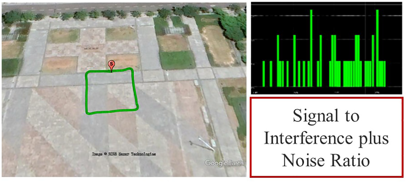
This study selected a carefully chosen open area with a strong GNSS signal during the test period of the testing platform vehicle to obtain comprehensive and representative data. In areas where UWB signals are adequately covered, UWB positioning accuracy is superior to that of GNSS. The selected field is situated at Boxue Square, South Lake Campus of Wuhan University of Technology, China, and its coordinates are latitude 30.51351339° and longitude 114.3284025°, based on the WGS-84 coordinate system. The onboard computer was programed to follow a specific driving route provided by high-precision RTK to obtain the relative position information of the testing platform vehicle.

The testing platform vehicle traveled along the predetermined route, starting from point S on the map as shown in Figure 8, while the onboard computer recorded the sensor data collected by the platform vehicle. Each collection lasted for 2 min, and a total of 10 data sets of GNSS, IMU, and UWB were collected. During the test period, the testing platform vehicle drove on multiple trajectories to obtain the best results. Two representative experimental data sets were selected for detailed analysis in this study.

Figure 8.

GNSS data.

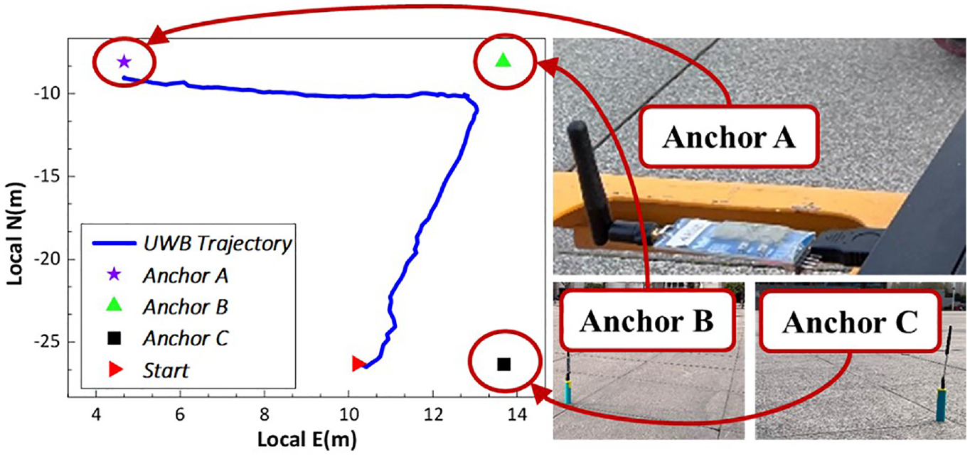
In this study, the GeographicLib library is utilized within the ROS framework for mathematical processing of geographic coordinates, including latitude, longitude, and altitude, and to convert GNSS data from the WGS-84 coordinate system to the North-East-Up coordinate system (NEU). The spatial arrangement of UWB anchors in the relative coordinate system is illustrated in Figure 9. Anchor A and B are positioned at coordinates (5, −8) and (14, −8), respectively, while anchor C is situated at (14, −20). Anchor A is situated at the endpoint, anchor B is parallel to A, and anchor C is perpendicular to B. This configuration is intended to facilitate the application of the Chan algorithm, which determines tag coordinates by computing the pseudoranges provided by each anchor. The layout also guarantees the UWB signal fully covers the target region and aids in determining coordinates when establishing the test site. The UWB reference trajectory, depicted by the blue trajectory in the figure, is generated by merging the pseudoranges measured by the test platform vehicle from each anchor upon entering the UWB signal range using the Chan algorithm. ³⁴ Additionally, the coordinate system of the UWB data is also the NEU coordinate system.

Figure 9.

UWB trajectory.

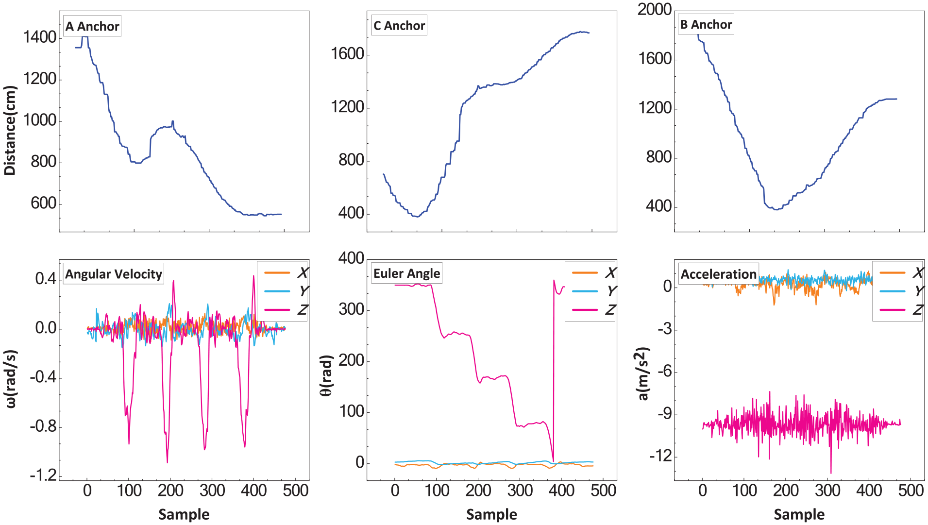
The experiment collected GNSS, UWB, and IMU data to assess the performance of the self-designed testing platform vehicle’s positioning. Figure 8 depicts the GNSS data collected during the experiment, with an average of 15 satellites used. On the other hand, Figure 10 displays the UWB and IMU data collected during the experiment, which includes the pseudorange of each anchor, three-axis acceleration, three-axis angular velocity, and three-axis Euler angles measured by the IMU. The system demonstrated normal collection of IMU and UWB data, with no data loss occurring during the test period. The results indicated that the positioning outcomes were consistent with the movement trajectory, and the UWB module was able to carry out distance measurement and positioning calculation functions effectively.

Figure 10.

Sensor raw data.

Typical environment experiment results

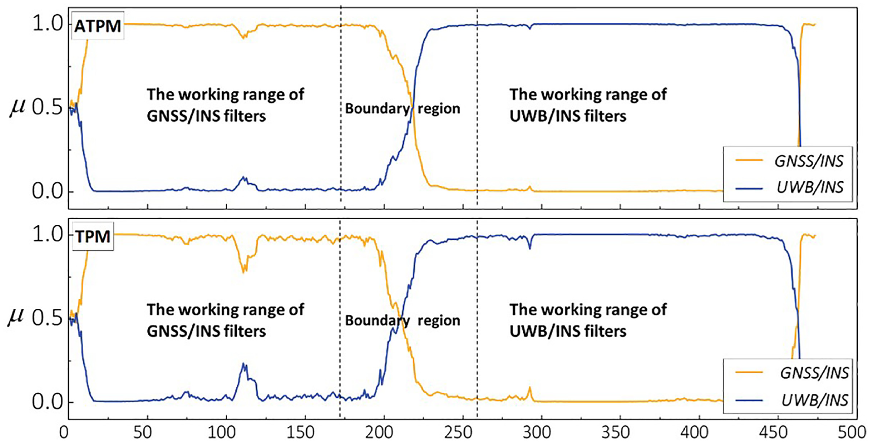
The model probability for the UWB/INS and GNSS/INS filter models were presented in Figures 11 and 12. The performance of the ATPM-IMM algorithm system was evaluated by analyzing the 278–464 data sampling points in case 1, and the results showed that it had a more stable model probability compared to the other filter models. In particular, the ATPM-IMM algorithm framework demonstrated its effectiveness in handling GNSS data blockage. In Figure 11, the system had to switch filters for the 25th sampling point due to the blockage, and the ATPM-IMM algorithm was able to complete the switching in a short time, demonstrating its agility and robustness in real-time applications.

Figure 11.

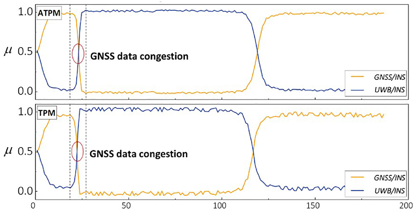
Case 1 model probability.

Figure 12.

Case 2 model probability.

In Figure 12, the changes in the model probability at data sampling points 70–145 in case 2 are illustrated. Within the framework of the IMM algorithm, it can be observed that after the 110th sampling point, the probability of the UWB/INS filter decreases gradually, while the probability of the GNSS/INS filter increases gradually. Moreover, as presented in Figure 18(b), the UWB/INS filter produces less error in the north direction than the GNSS/INS filter. Therefore, the ATPM-IMM algorithm system framework opts to maintain the model probability of the UWB/INS filter. From this analysis, it is evident that the ATPM-IMM algorithm demonstrates superior tracking capabilities.

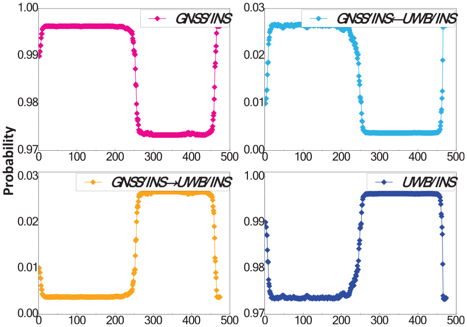
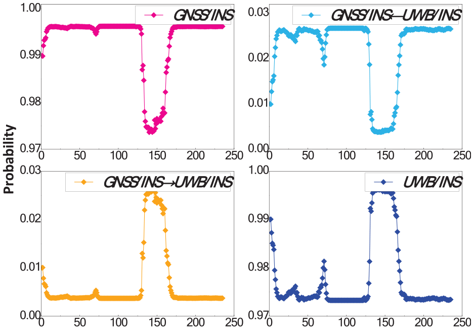
The figure depicted in Figures 13 and 14 illustrates the dynamic changes in the transition probabilities of the state transition matrix, which were obtained using the ATPM-IMM algorithm framework. These transition probabilities show a closer correlation with the trends observed in ATPM-IMM model probability. Specifically, the probabilities captured in this analysis encompass the likelihood of maintaining the current GNSS/INS filter, the probability of switching from the UWB/INS filter to the GNSS/INS filter, the probability of switching from the GNSS/INS filter to the UWB/INS filter, and the likelihood of retaining the current UWB/INS filter. In case 2, as the GNSS/INS filter error increases, the system increases the probability of switching to the UWB/INS filter, and maintains the probability of UWB/INS filter.

Figure 13.

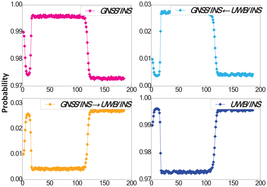
Case 1 transition probability.

Figure 14.

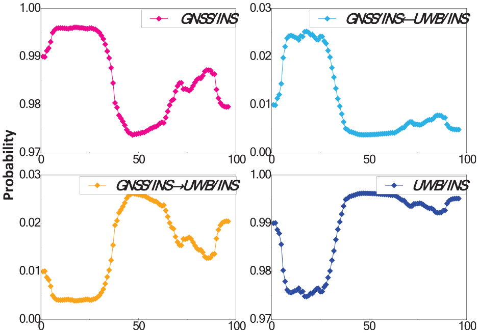
Case 2 transition probability.

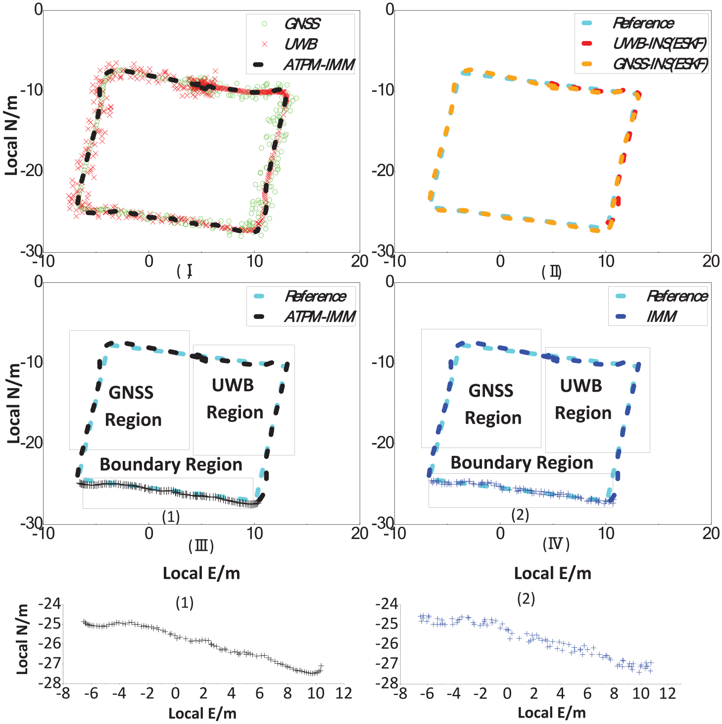
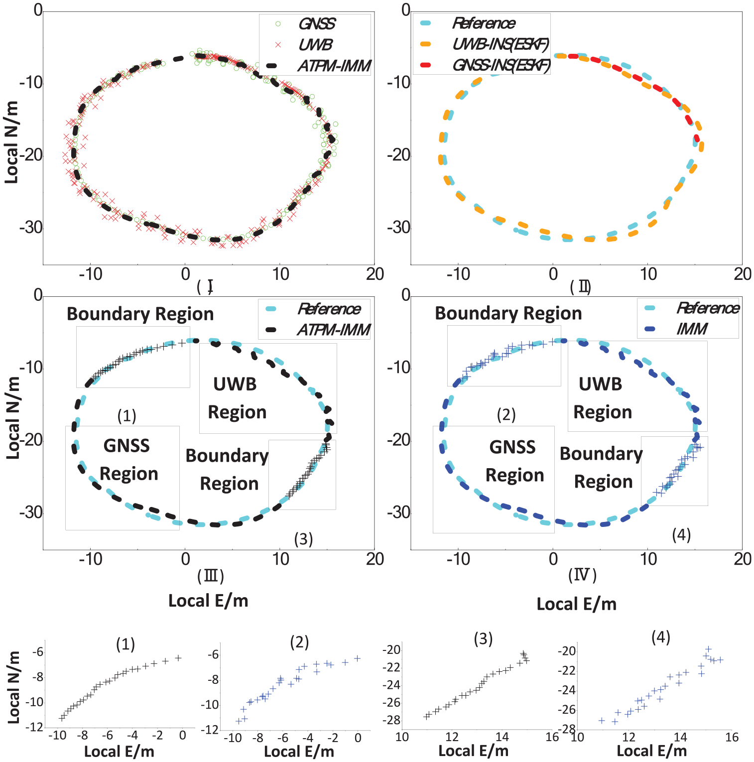
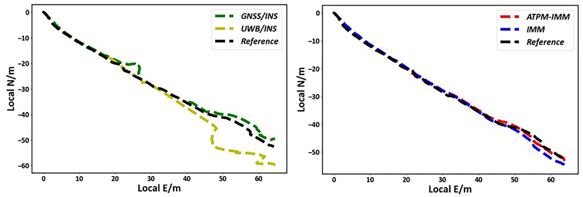
Figures 15 and 16 demonstrate the comparison of motion trajectories for case 1 and case 2. Figures 15(I) and 16(I) respectively exhibit the motion trajectory of the testing platform vehicle acquired using the ATPM-IMM algorithm and the pure UWB and GNSS solutions. Figures 15(II) and 16(II) show the motion trajectory obtained by fusion using the ESKF algorithm. Additionally, Figures 15(III), 16(III), 15(IV), and 16(IV) demonstrate the motion trajectories calculated by the ATPM-IMM algorithm and IMM algorithm, respectively. Based on the analysis presented in the figure, it can be concluded that the ATPM-IMM algorithm can select the optimal matching filter for the current system motion state by adjusting the model probability.

Figure 15.

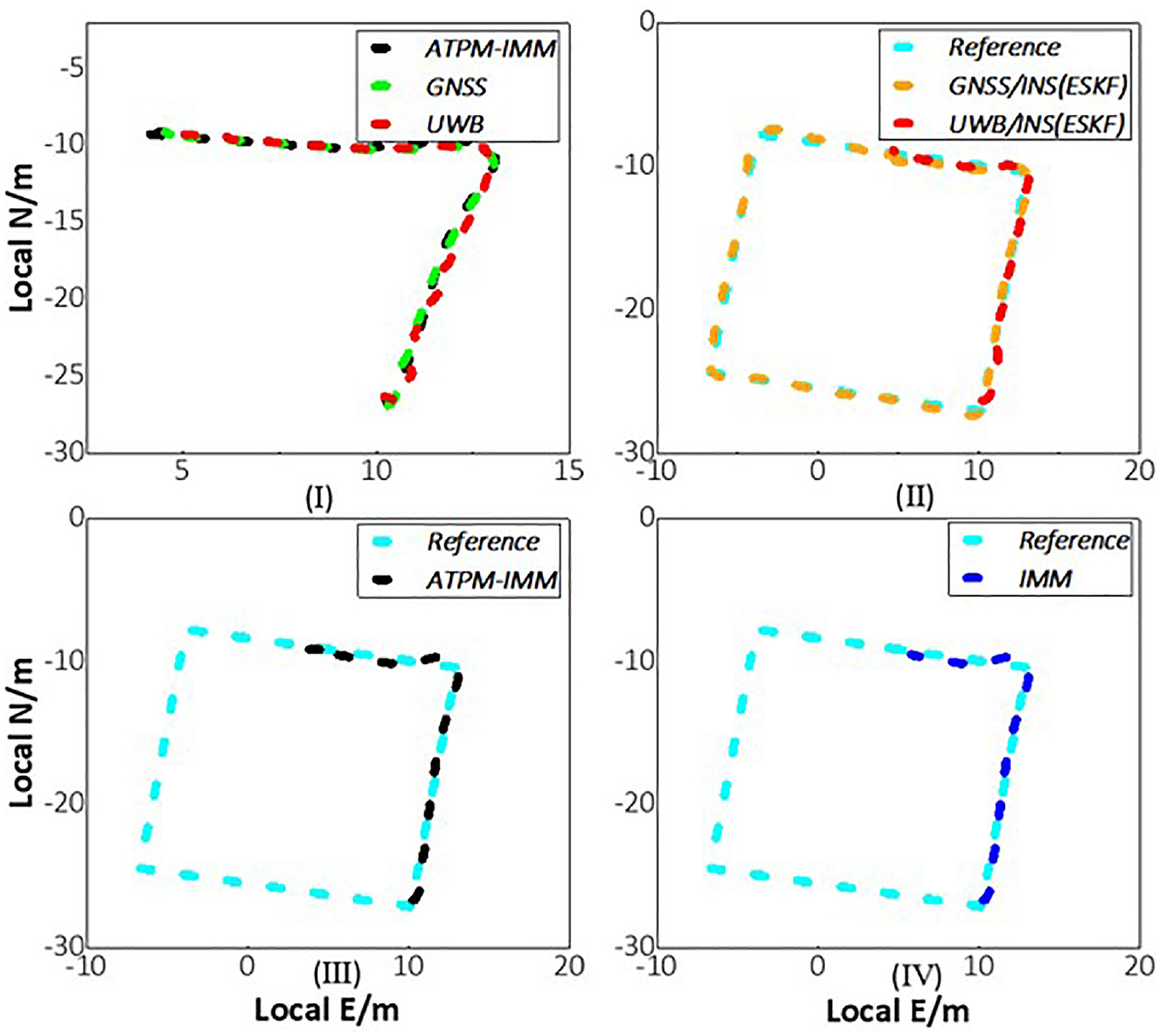
Case 1 motion trajectory.

Figure 16.

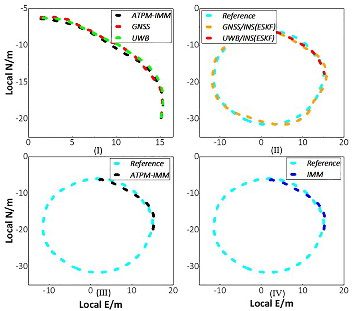
Case 2 motion trajectory.

In this study, as shown in Figures 17 and 18, the magnitude and distribution of the errors in the east and north directions for three different algorithms during the vehicle navigation process are presented. To display the error values, the absolute value of the difference between the reference trajectory and the algorithm solution trajectory is used. In the process of integrated navigation, the model probability of each local system is switched in real-time, which can establish the most accurate model to describe the present state of the local system. As shown in Figure 17(a), the trajectory of the testing vehicle is at one corner of the quadrilateral. Due to signal delay, the eastward error of the UWB/INS filter jumps at the 353rd and 403rd sample points, while the GNSS/INS filter maintains a relatively low level of error.

Figure 17.

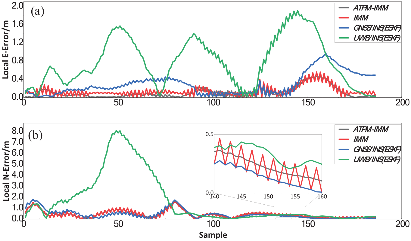
(a) Case 1 error distribution in east direction and (b) Case 2 error distribution in east direction.

Figure 18.

(a) Case 2 error distribution in north direction and (b) Case 2 error distribution in north direction.

In case 2, as shown in Figure 18(a), the northward error of the UWB/INS filter shows a downward trend at the 110th sample point. The ATPM-IMM algorithm tracks the UWB/INS filter, while the IMM algorithm increases the weight of the GNSS/INS filter, resulting in an overall increase in the system’s error in the north direction. It can be seen from the error jump that the ATPM-IMM algorithm is superior to the traditional IMM algorithm in reducing the overall error. From the distribution and magnitude of the errors, it can be seen that the ATPM-IMM algorithm can accurately select the current system matching model and improve the accuracy of the positioning system.

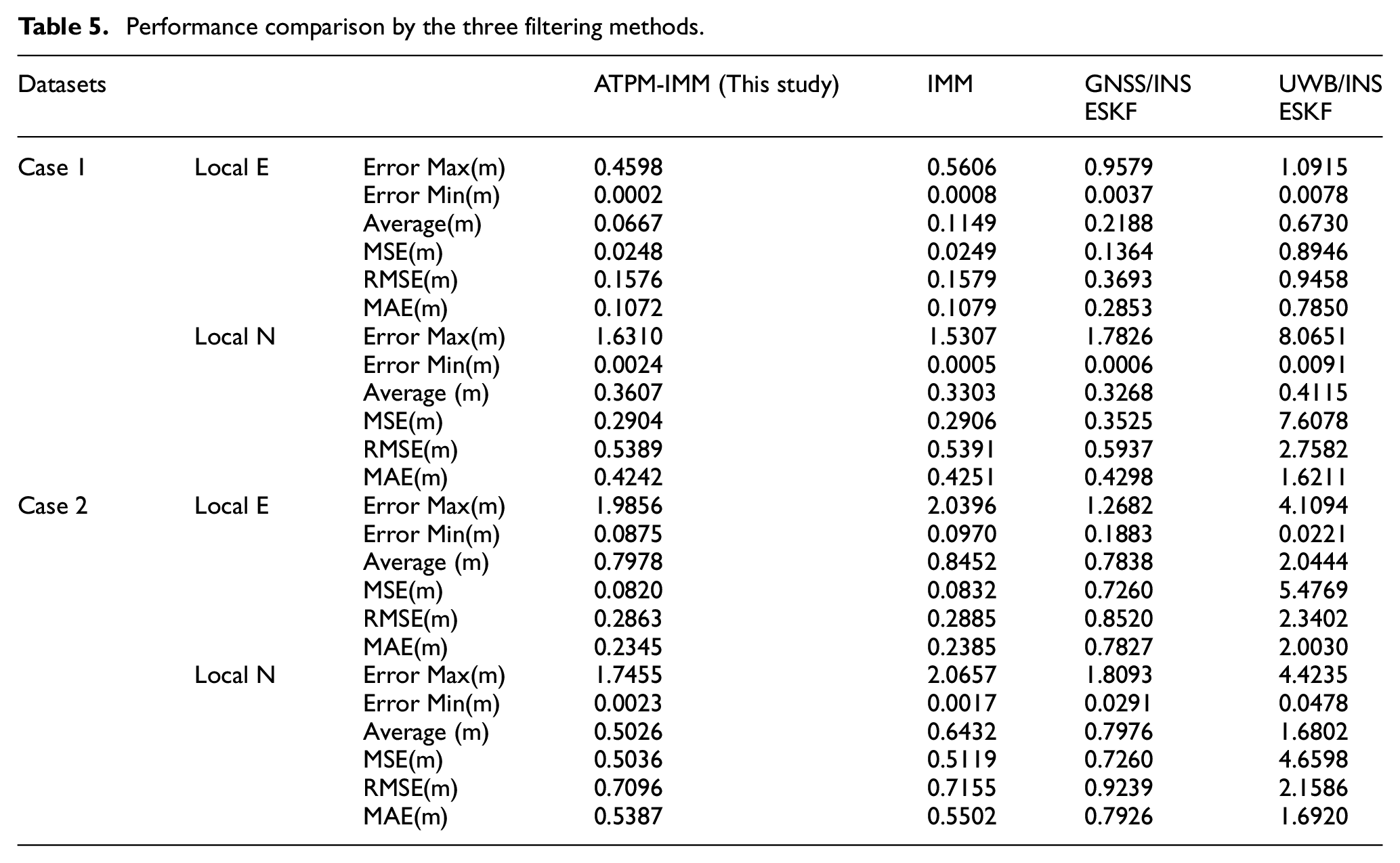
Based on the outcomes presented in Figures 19 and 20 and Table 5, it can be inferred that the ATPM-IMM algorithm outperforms the ESKF in terms of position error in the combined navigation experiment of the testing platform vehicle. Specifically, the optimization effect of the ATPM-IMM algorithm is 5.4% higher than that of the IMM algorithm, 31.17% higher than that of the single GNSS/INS filter, and 41.23% higher than that of the single UWB/INS filter, considering the average value of the error and other indicators. The results of the position error in the vehicle-mounted combination navigation experiment further demonstrate that the proposed ATPM-IMM system framework can effectively enhance the accuracy of combined navigation and has significant advantages compared to the IMM algorithm and dual-sensor filter.

Figure 19.

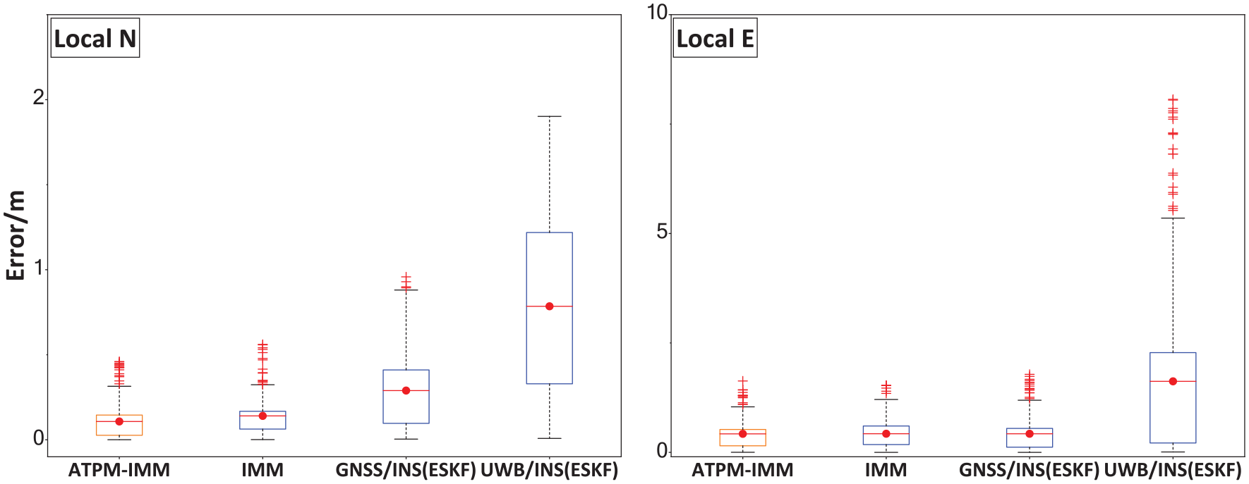
Case 1 error box-plot.

Figure 20.

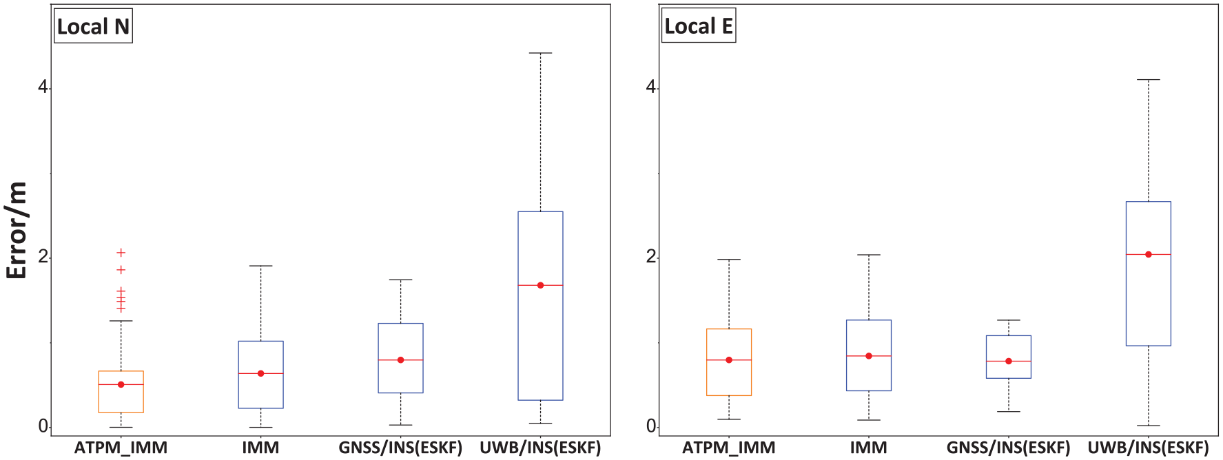
Case 2 error box-plot.

Table 5.

Performance comparison by the three filtering methods.

Datasets			ATPM-IMM (This study)	IMM	GNSS/INSESKF	UWB/INSESKF
Case 1	Local E	Error Max(m)	0.4598	0.5606	0.9579	1.0915
		Error Min(m)	0.0002	0.0008	0.0037	0.0078
		Average(m)	0.0667	0.1149	0.2188	0.6730
		MSE(m)	0.0248	0.0249	0.1364	0.8946
		RMSE(m)	0.1576	0.1579	0.3693	0.9458
		MAE(m)	0.1072	0.1079	0.2853	0.7850
	Local N	Error Max(m)	1.6310	1.5307	1.7826	8.0651
		Error Min(m)	0.0024	0.0005	0.0006	0.0091
		Average (m)	0.3607	0.3303	0.3268	0.4115
		MSE(m)	0.2904	0.2906	0.3525	7.6078
		RMSE(m)	0.5389	0.5391	0.5937	2.7582
		MAE(m)	0.4242	0.4251	0.4298	1.6211
Case 2	Local E	Error Max(m)	1.9856	2.0396	1.2682	4.1094
		Error Min(m)	0.0875	0.0970	0.1883	0.0221
		Average (m)	0.7978	0.8452	0.7838	2.0444
		MSE(m)	0.0820	0.0832	0.7260	5.4769
		RMSE(m)	0.2863	0.2885	0.8520	2.3402
		MAE(m)	0.2345	0.2385	0.7827	2.0030
	Local N	Error Max(m)	1.7455	2.0657	1.8093	4.4235
		Error Min(m)	0.0023	0.0017	0.0291	0.0478
		Average (m)	0.5026	0.6432	0.7976	1.6802
		MSE(m)	0.5036	0.5119	0.7260	4.6598
		RMSE(m)	0.7096	0.7155	0.9239	2.1586
		MAE(m)	0.5387	0.5502	0.7926	1.6920

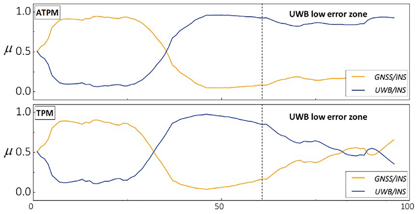
Typical environment algorithm adaptability

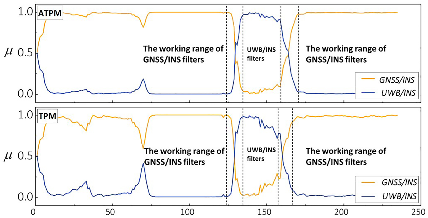
To evaluate the superior performance of the ATPM-IMM algorithm in achieving seamless navigation, the present study incorporated white noise with a mean of 0 and variance of 0.1 to the latitude and longitude data obtained by the GNSS sensor in two experiments. The GNSS data was gathered 278–464 sampling points in case 1 and 70–145 sampling points in case 2 within the UWB signal area. The data from the GNSS, UWB, and IMU sensors were then fed into the ATPM-IMM algorithm to compute the motion trajectory of the testing platform vehicle. In case 1, the first 278 sampling points are shown in Figure 21. The testing platform vehicle does not enter the UWB signal coverage area, so the GNSS/INS filter was the main positioning method, and the filter worked in the 278–464 sampling points and switched back to the GNSS/INS filter in the 464–475 sampling points. In the 125 sampling points of case 2, as shown in Figure 22, the main matching model of the system was the GNSS/INS filter, the filter worked in the 125–175 sampling points, and then switched back to the GNSS/INS filter. It can be seen from the figure that the confidence of the filter matching the current system state in the ATPM-IMM algorithm is relatively stable compared to the TPM algorithm in the 100–150 sampling points of Figure 21 and the first 125 sampling points of Figure 22. In the 200–250 sampling points of Figure 21 and the 150–175 sampling points of Figure 22, the model switch is smoother than that of the TPM algorithm.

Figure 21.

Case 1 model probability.

Figure 22.

Case 2 model probability.

Figures 23 and 24 illustrates the fluctuation pattern of the state transition matrix’s transition probabilities within the ATPM-IMM algorithm framework while operating in a single filter working state. The dynamics of these probabilities are highly correlated with the evolution of the ATPM-IMM model probability, as discussed in depth in Section 3.4 of the manuscript. It can be observed that when entering the effective range of GNSS or UWB, the corresponding model transition probability increases toward the model that aligns with the current system state.

Figure 23.

Case 1 seamless transition probability.

Figure 24.

Case 2 seamless transition probability.

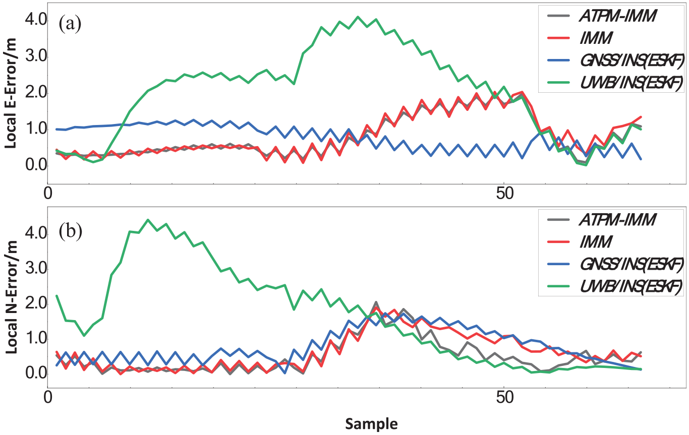
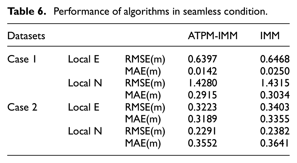
As depicted in Figures 25 and 26, the figures showcase the motion trajectory of the experimental vehicle, where ESKF, IMM, and ATPM-IMM algorithms are employed in the presence of white noise. Furthermore, the performance of the IMM and ATPM-IMM algorithms at the GNSS/INS filter and UWB/INS filter junction are also analyzed. In the rectangular trajectory of case 1, the ATPM-IMM algorithm displays a more precise trend analysis of the increasing errors in the GNSS/INS filter and decreasing errors in the UWB/INS filter, compared to the IMM algorithm. The ATPM-IMM algorithm generates coordinate points with a more uniform distribution and less scatter. The root mean square error in the east direction of the ATPM-IMM algorithm is 0.6397, which is smaller than that of the IMM algorithm (0.6468), as shown in Table 6. In the circular trajectory of case 2, the vehicle encounters two switches between the GNSS/INS and UWB/INS filters and eventually re-enters the GNSS signal range. In this case, both the northward and eastward error distributions of the ATPM-IMM algorithm are smaller than those of the IMM algorithm, as also highlighted in Table 6. The ATPM-IMM algorithm can accurately detect the trend of increasing errors in the GNSS/INS filter and decreasing errors in the UWB/INS filter, as well as the trend of decreasing errors in the GNSS/INS filter and increasing errors in the UWB/INS filter, effectively reducing the scatter of points at the model switching.

Figure 25.

Case 1 seamless motion trajectory.

Figure 26.

Case 2 seamless motion trajectory.

Table 6.

Performance of algorithms in seamless condition.

Datasets			ATPM-IMM	IMM
Case 1	Local E	RMSE(m)	0.6397	0.6468
		MAE(m)	0.0142	0.0250
	Local N	RMSE(m)	1.4280	1.4315
		MAE(m)	0.2915	0.3034
Case 2	Local E	RMSE(m)	0.3223	0.3403
		MAE(m)	0.3189	0.3355
	Local N	RMSE(m)	0.2291	0.2382
		MAE(m)	0.3552	0.3641

Figures 27 and 28 shows the errors of the ATPM-IMM and IMM algorithms compared to the reference trajectory of the testing vehicle in the two experiments. From the figure, it can be observed that the ATPM-IMM algorithm has a similar trend in error changes as the IMM algorithm, but with smaller fluctuations. The IMM algorithm exhibits larger fluctuations and better error stability than the ATPM-IMM algorithm. In the filter switching region, the ATPM-IMM algorithm exhibits smaller fluctuations and more stable weight adjustment than the IMM algorithm. As a positioning algorithm system for the testing platform vehicle, considering the importance of driving a predetermined route in conjunction with other test vehicles, the use of the ATPM-IMM algorithm would be more ideal for ensuring error stability.

Figure 27.

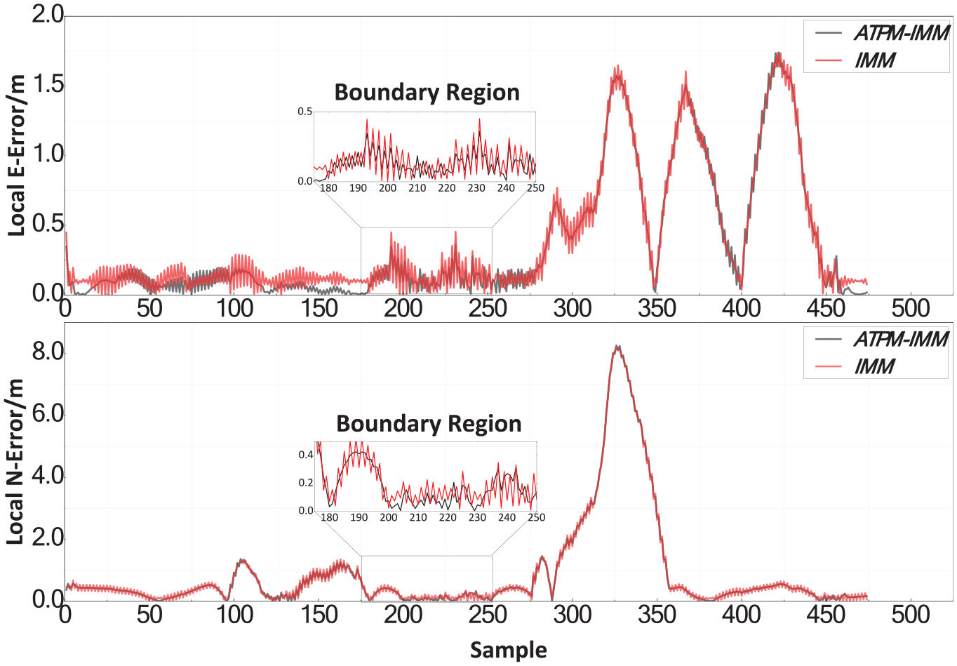
Case 1 seamless error distribution.

Figure 28.

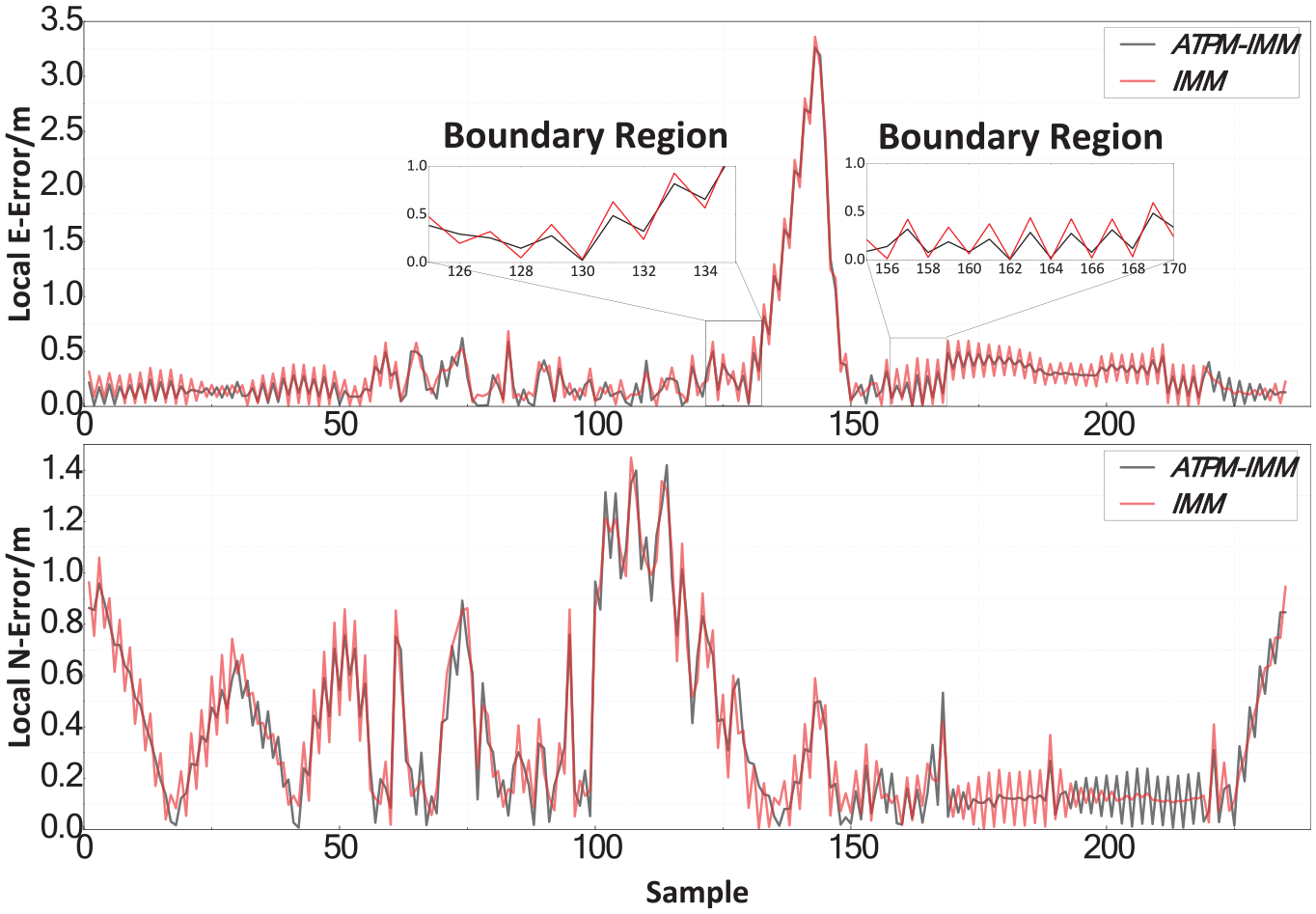
Case 2 seamless error distribution.

Challenging environment experiment

To further verify the smoothness and robustness of the proposed algorithm during model switching, as well as the accuracy of the positioning results, this study included experiments in challenging environment. A location within the school where GNSS signals are obstructed was selected, with coordinates at latitude 30.51200075° and longitude 114.3323483°. As illustrated in Figures 29 and 30, the GNSS signal is lost when the testing platform vehicle passes beneath the skybridge between two tall buildings, due to obstruction by the buildings. However, as the vehicle exits this area, the GNSS signal is restored, and the GNSS trajectory on the map is correspondingly reestablished. In the region where the GNSS signal is lost, four UWB anchors were strategically placed, as illustrated in the lower left of Figures 29 and 30. This setup ensures that UWB signals adequately cover the area where GNSS signals are obstructed, thereby enabling the use of UWB for accurate positioning in scenarios where GNSS signals are unavailable.

Figure 29.

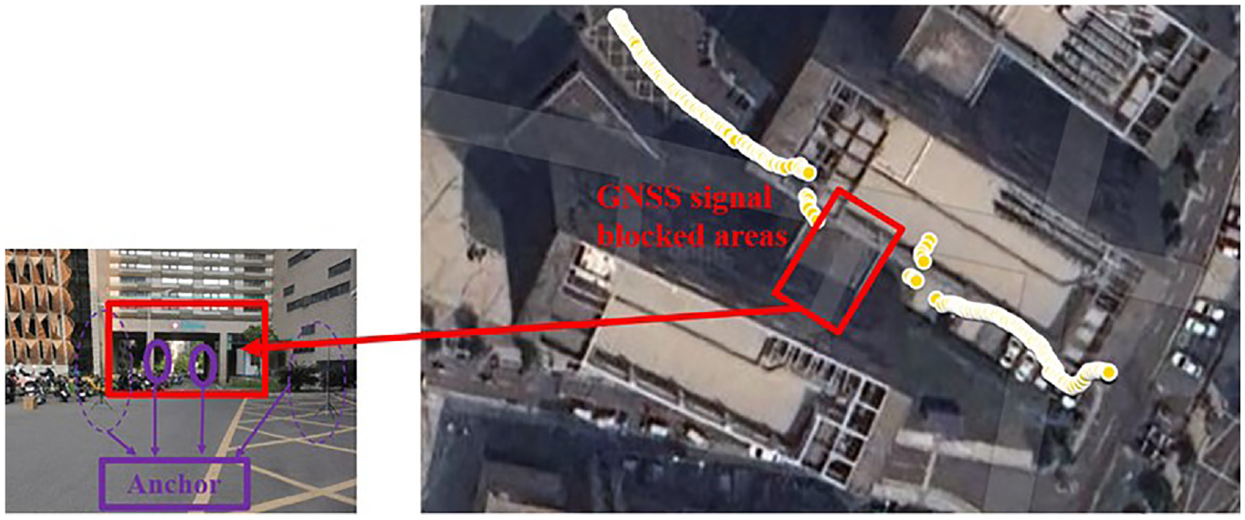
Challenging environment experiment diagram.

Figure 30.

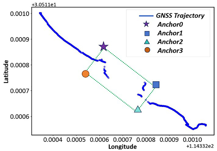
GNSS trajectory and UWB anchor layout.

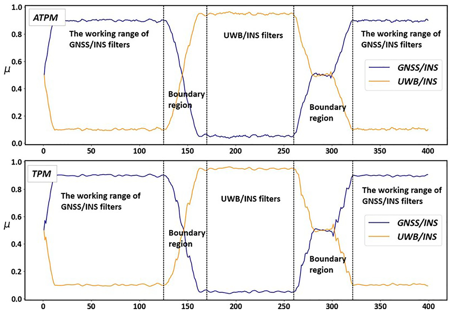
To evaluate the superior performance of the ATPM-IMM algorithm in achieving seamless navigation, we selected GNSS data and UWB data collected in challenging environment for fusion. As shown in Figure 31, both GNSS and UWB data were sampled during the 0–130 sampling points, with the system’s main filter being the GNSS/INS filter. During 130–160 sampling points, due to building obstructions, the GNSS signal was affected until completely lost, at which point both filters operated simultaneously. During 160–260 sampling points, with the GNSS signal lost, the UWB/INS became the system’s main filter. During 260-320 sampling points, as the GNSS signal was restored, the filter transitioned from the UWB/INS filter back to the GNSS/INS filter. Afterward, as the testing platform vehicle moved away from the UWB anchor 2 and 3, the system’s main filter was the GNSS/INS filter. It can be seen from the figure that during the 130–160 and 260–330 sampling points, the ATPM-IMM algorithm demonstrated more stable confidence in filter matching the current state compared to the TPM algorithm, correspondingly showing that ATPM-IMM achieves smoother model transitions in actual challenging environment.

Figure 31.

Model probability in challenging environment.

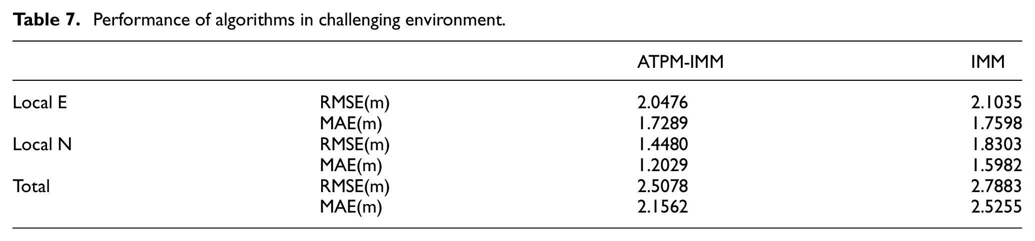
As depicted in Figure 32, the GNSS/INS trajectory disconnects when GNSS signal is lost and reappears when the signal is restored. In the actual trajectory, the ATPM-IMM algorithm demonstrates a more accurate distribution trend compared to the IMM algorithm, with the ATPM-IMM trajectory aligning more closely with the real trajectory. As shown in Figures 33 and 34, the errors in the eastward, northward, and overall directions are smaller for the ATPM-IMM algorithm than for the IMM algorithm. According to Table 7, the northward error of the ATPM-IMM algorithm is reduced by 2.6%, the eastward error by 20.88%, and the overall positional error by 10.05% compared to the IMM algorithm. When re-entering the operational area of the GNSS/INS filter for the second time, the ATPM-IMM algorithm is closer to the real trajectory in both the eastward and northward directions, hence ATPM-IMM achieves more accurate and quicker filter transitions than the IMM algorithm. Figure 35 shows the error comparison between the ATPM-IMM and IMM algorithms and the reference trajectory of the testing vehicle in a challenging environment. It is evident that both algorithms have similar overall error distribution trends. However, during the second switch from UWB/INS to GNSS/INS filters, the northward error change trend of ATPM-IMM is smaller compared to IMM, demonstrating better error stability of the ATPM-IMM algorithm. Therefore, in actual challenging environments, ATPM-IMM exhibits better accuracy and environmental adaptability and can be prioritized as the algorithm for the testing platform vehicle.

Figure 32.

Seamless motion trajectory in challenging environment.

Figure 33.

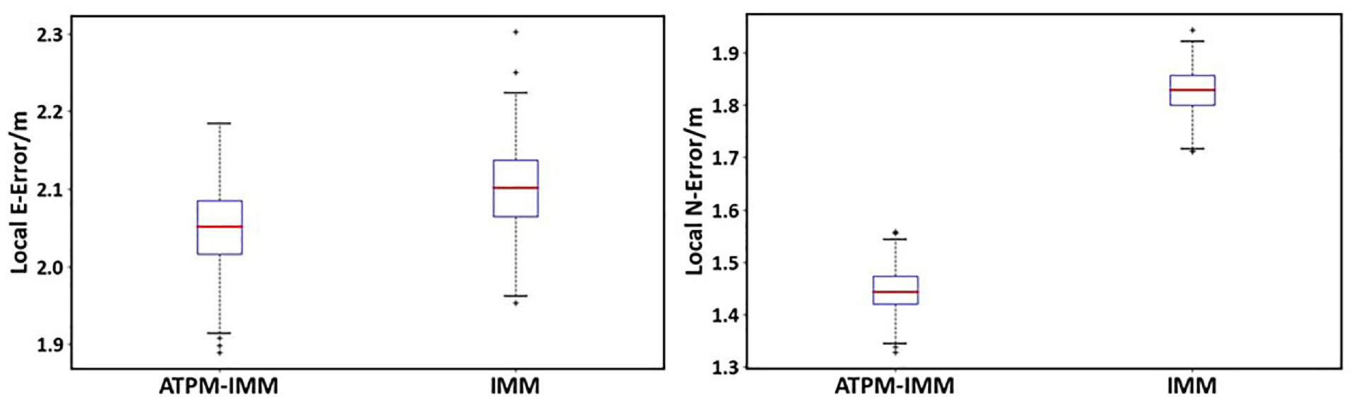
Error box-plot in challenging environment.

Figure 34.

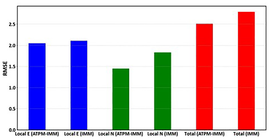
Error RMSE histogram in challenging environment.

Table 7.

Performance of algorithms in challenging environment.

		ATPM-IMM	IMM
Local E	RMSE(m)	2.0476	2.1035
	MAE(m)	1.7289	1.7598
Local N	RMSE(m)	1.4480	1.8303
	MAE(m)	1.2029	1.5982
Total	RMSE(m)	2.5078	2.7883
	MAE(m)	2.1562	2.5255

Figure 35.

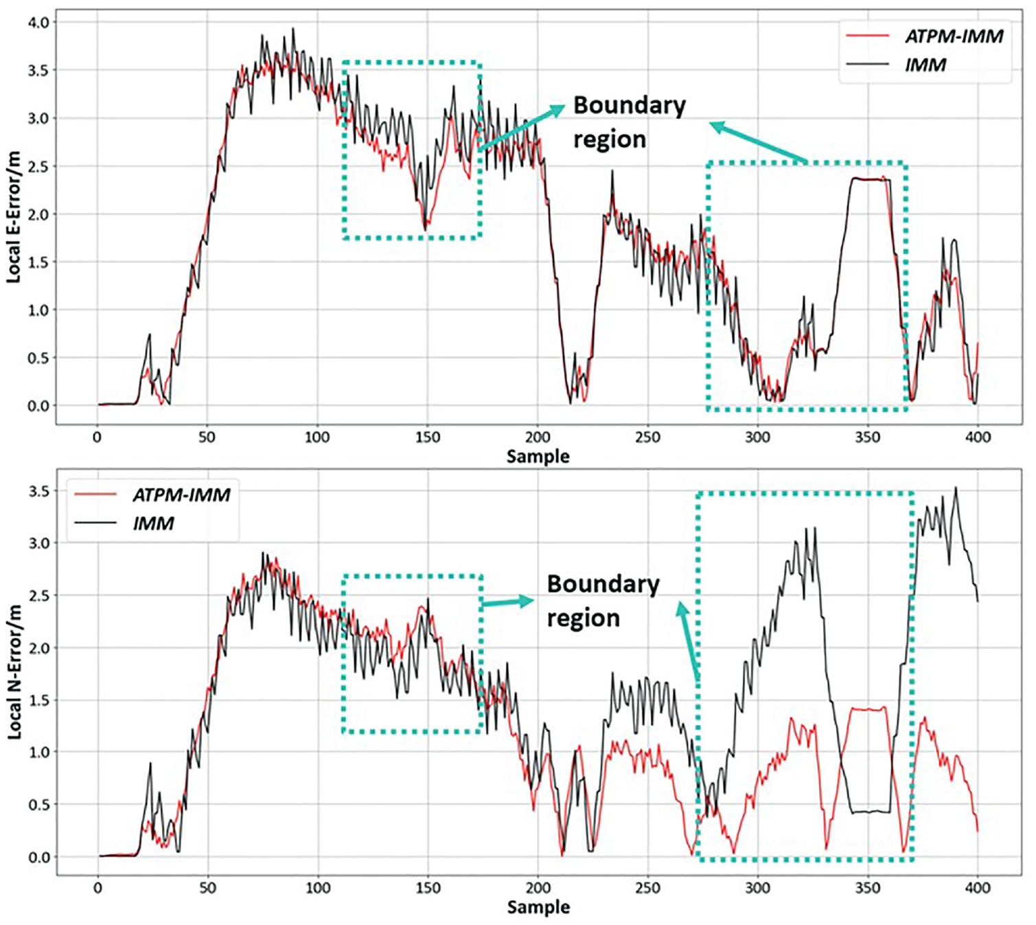
Seamless error cistribution in challenging environment.

Conclusion

This study proposes an advanced ATPM-IMM algorithm, on the basis of IMM, that is designed for low-cost and compact sensor integration for UWB/IMU/GNSS navigation and positioning in an ADAS testing platform vehicle. The proposed algorithm is dependent on probability rate correction to enhance the accuracy of the current system state model matching and to enhance the robustness of the algorithm in comparison with the IMM algorithm. The ATPM-IMM algorithm seamlessly switches to another filter in the event of a single filter failure, thus improving navigation and positioning accuracy in a multi-sensor working environment.

The effectiveness of the ATPM-IMM algorithm was rigorously tested on the ADAS testing platform using real vehicle data. In ordinary environments, the ATPM-IMM algorithm improved navigation accuracy by 5.4% compared to the IMM algorithm. It also demonstrated significant improvements over single GNSS/INS ESKF and single UWB/INS ESKF, with accuracy enhancements of 31.17% and 41.23%, respectively. In more challenging environments, the ATPM-IMM algorithm increased navigation accuracy by 10.05% compared to the IMM algorithm. This algorithm effectively minimizes data drift at model boundaries, resulting in smoother computational outcomes in single filter operations. By utilizing an adaptive model transition probability correction method based on measurement data, the impact of matching models is amplified while that of non-matching models is diminished. Moreover, it ensures reliable model tracking even in the presence of substantial system errors or failures, thereby enhancing the effectiveness of matching models and mitigating the effects of model mismatches.

While the algorithm satisfies the requirements for real-time, low-frequency navigation, it necessitates further improvements to adeptly handle high-frequency dynamic scenarios. Future research will focus on devising methods to efficiently address these high-frequency dynamic environments, expanding the testing scope of the algorithm, and broadening its applicability to diverse fields.