Sage Journals: Discover world-class research

Abstract

In this study, we introduce a novel algorithm, the low error rate adaptive fading Kalman filter (LERAFKF), designed to predict system states in the presence of uncertainty in both the system matrix and the model. The purpose of developing the LERAFKF is to address challenges arising from measurement difficulties, system parameter uncertainties, and state–space model inaccuracies. Several studies have utilized the Kalman filter (KF) and extended Kalman filter (EKF) algorithms to handle uncertainties in system parameters, corrupted measurements with unknown covariances, and incorrectly defined system modeling. Our work distinguishes itself by proposing a new approach that achieves lower error and deviation rates by combining the current Kalman estimation algorithm and the fading factor adaptive filter. To achieve this goal, we transformed the KF into an adaptive KF by introducing a forgetting factor, and the algorithm was subsequently reconfigured to calculate an optimized forgetting factor. In this study, we conducted simulations and measurements using both linear and nonlinear systems. The linear system represents the motion of an object, and the simulation involved measurements from the inertial navigation system (INS) sensor, specifically the Pololu IMU01b three-axis inertial measurement unit (IMU) sensor. We employed the SDI33 system with 9 degrees of freedom (DoF) mounted on a three-axis rotary table for the nonlinear system. This system simulates a missile as a 4th-order nonlinear system. Our findings demonstrate that the proposed LERAFKF filter outperforms KF and EKF in estimating system states, particularly in measurement-related error scenarios. Mean square error analysis further confirmed that LERAFKF exhibited the lowest error values, showcasing superior performance over KF and EKF in linear and nonlinear systems.

Keywords

State–space model adaptive Kalman filter low error rate adaptive fading Kalman filter

Introduction

GNSS provides highly accurate positioning information at frequency bands as low as 1 Hz. However, GNSS performance can be compromised by the need for a clear line of sight to satellites. Factors such as multipath propagation in dense urban environments, interference, signal clutter, misalignment, or intentional denial of full service can adversely impact GNSS effectiveness.^1,2 In contrast, an inertial navigation system (INS) operates as a standalone system, providing navigation information at a high measurement rate without reliance on external sources. A significant challenge is the accumulation of errors over time.³ Furthermore, microelectronic mechanical systems (MEMS)-based inertial measurement units, with inherent faults like constant shift, scale factor, bias, and non-orthogonality, contribute to noise and uncertainty in their output.⁴ Particularly when GNSS is non-functional or disabled, it becomes imperative to implement measures to enhance the robustness of navigation algorithms and compensate for sensor errors.⁵ Consequently, problems arise in prediction algorithms aiming to predict future states accurately owing to the accumulation of errors over time.⁶

The Kalman filter (KF) is robust when system parameters are precisely known. However, in scenarios where the system characteristics are inadequately characterized, the filter’s estimation performance is significantly affected.^7–9

In this context, the first study conducted by Kalman in 1960¹⁰ marked the emergence of examples addressing the estimation problem.

Mehra¹¹ continued this work in 1971, focusing on the linear model. Subsequent studies between 1972 and 1999 aimed at rectifying errors in the KF.

The introduction of the forgetting factor gained prominence in 1988 through studies by Lee¹² and later by Xia and Shen in 1994.¹³ Nevertheless, further advancements in this field were necessary.

Studies on the system resulting from inertial navigation system (IMU) sensor measurements gained momentum in 2001 with Bar-Shalom et al.¹⁴ and later in 2004 with Titterton and Weston.⁴

Hide et al.¹⁵ studied velocity and acceleration estimation using a low-cost INS with the KF.

El-Sheimy et al.¹⁶ conducted modeling and analysis using the Allan variance method with inertial sensors.

Ding et al.¹⁷ focused on enhancing estimation results through an integrated GNSS/INS model.

Ngoc et al.¹⁸ conducted position improvement studies exclusively with GNSS, experimenting with process noise and measurement noise on the model.

Faragher¹⁹ provided a straightforward derivation of the KF handling two Gaussian functions simultaneously, simplifying the result to a compact form.

Bou et al.²⁰ recommended the multiple fading factors KF algorithm to increase the error variance matrix of the one-step prediction of the state estimation. Kai Wei et al.²¹ compared the adaptive KF and traditional extended Kalman filter (EKF) in selecting the update measurement noise matrix R and/or the process noise matrix Q. The selection was based on the maximum likelihood criterion and Kalman gain factors.

Takaki and Nobuaki²² argued that implementing an adaptive EKF enhanced the accuracy of global navigation satellite system position, velocity, and time and their integrity information through single-point positioning in dense urban environments, all achieved without sensor aiding or coupling.

The most critical issues in these studies include minimizing prediction deviation with low error when relying solely on INS during GPS disconnection and testing this scenario using data from a widely employed IMU sensor. Limited research on this topic may be attributed to commercial considerations, or relevant findings might not have been publicly disclosed. This study introduces a low error rate adaptive fading Kalman filter (LERAFKF) algorithm for predicting state–space system states. The algorithm employs an adaptive form of the scalar forgetting factor. This paper is structured as follows. Section “Kalman filter and extended Kalman filter estimation algorithm” provides a summary of the fundamentals of KF and EKF. Our proposed method is detailed in section “Adaptation of Kalman filter with low error rate fading factor.” Section “Simulation results” presents simulation results with implementation specifics. Section “Conclusion” concludes the paper by highlighting the advantages of the proposed algorithm over LERAFKF and suggesting potential avenues for further research to address encountered problems.

Kalman filter and extended Kalman filter estimation algorithm

The KF algorithm primarily consists of two models: a process model outlining the evolution of system states over time and a measurement model detailing the acquisition of measurements from the process, particularly when dealing with noisy or erroneous measurements. The system is subsequently characterized by state and output equations, denoted by equations (1) and (2), respectively.^23–26

x_{k} = Φ_{k - 1} x_{k - 1} + G_{k - 1} w_{k - 1}

(1)

y_{k} = H_{k} x_{k - 1} + v_{k}

(2)

Here, $x_{k} \in R^{n}$ is the state vector, and $y_{k} \in R^{m}$ is the measurement (system output) vector. $Φ_{k}, G_{k}, H_{k}$ are state transition matrices with nxn, nxp, and mxn dimensions, respectively. $w_{k}$ is a p-dimensional Gaussian white noise sequence, and $v_{k}$ is an m-dimensional Gaussian white noise sequence.

The state estimation starts with the initial value $x_{0}$ and initial error covariance $P_{0}$ . The description of the error covariance, the Kalman gain, and the recursive state estimates are summarized in equations (3)–(5), as provided below.

P_{k / k - 1} = Φ_{k - 1} P_{k - 1} Φ_{k - 1}^{T} + G_{k - 1} Q_{k - 1} G_{k - 1}^{T}

(3)

K_{k / k - 1} = P_{k / k - 1} H_{k}^{T} (H_{k} P_{k / k - 1} H_{k}^{T} + R_{k})^{- 1}

(4)

{\overset{\land}{x}}_{k} = {\overset{\land}{x}}_{k / k - 1} + K_{k} (y_{k} - H_{k} {\overset{\land}{x}}_{k / k - 1})

(5)

Here, $P_{k}$ is the covariance matrix, $K_{k}$ is the Kalman gain, and ${\overset{\land}{x}}_{k}$ represents the state estimate. $Q_{k}$ and $R_{k}$ are the process noise and measurement noise covariances, respectively.

In this process, the state variables undergo correction at each step through the multiplication of the Kalman gain by the difference between the measured output value of the system and the output value computed using the preceding state variable in the system model. The Kalman gain, acting as an input to the model, dynamically adapts to improve subsequent predictions.²⁴ The KF demonstrates exceptional predictive performance when the noise affecting the system parameters is statistically well-modeled.^11,12 Prediction errors within the KF are categorized into two scenarios: the first involves defects in the model, while the latter encompasses measurement flaws. Traditionally, precise, calibrated instruments are employed to establish the covariance matrix for modeling noise. However, owing to noise’s time, space, and sensor-dependent nature, determining when and how changes occur can be challenging.²² For an accurate estimate, determining the values of the Q and R matrices becomes critical. Higher values for the R matrix are chosen if issues are expected in the measurements. In contrast, relatively higher values for the Q matrix are chosen if problems in the system modeling are anticipated.²⁷

Numerous scenarios involve nonlinear system behavior, rendering the conventional KF ineffective for accurate estimation. The EKF is a nonlinear filter variant of the KF designed to estimate the states of nonlinear systems. Equation (6) represents the nonlinear model of the physical system.²⁸

x_{k} = f (x_{k - 1}, u_{k - 1}) + w_{k - 1}

(6)

The nonlinear form of the measurement model is represented by equation (7) for the discrete form.

y_{k} = h (x_{k}) + v_{k}

(7)

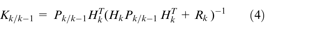
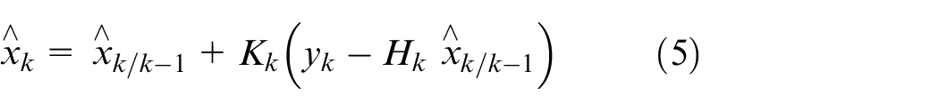
The prediction step of EKF covariance is determined by equation (8). The posterior state and Kalman gain are calculated using the methodology outlined in equations (4) and (5).

P_{k / k - 1} = Φ_{k} P_{k - 1} Φ_{k}^{T} + Q_{k - 1}

(8)

When the system states and measurement equation exhibit nonlinearity, the probability distribution of the states becomes non-Gaussian. Consequently, this non-Gaussian distribution has covariance matrices that cannot describe the states. To address this, the EKF uses the current estimated states as a reference point, around which the state transition and measurement models are linearized using their respective Jacobians.²⁹

Adaptation of Kalman filter with low error rate fading factor

The KF works successfully if it accurately includes the system dynamics to be estimated. However, incorrect prior values and unknowns in the system and observation matrices can lead to inaccurate predictions or even divergence during the filter’s operation. Adaptive filters, essential in such scenarios, aim to mitigate errors and divergence issues.²² To solve this problem in linear systems, some algorithms have been used to make the KF adaptive.^17–21 Adaptive KF studies generally fall into three categories: correct determination of the covariance matrix, robust measures against measurement errors, and strategies to handle unknown parameters in the state matrix. Various approaches have been explored, with one notable method being the adaptive KF with a fading factor. In this filter, the fading factor emphasizes recent measurements and reduces the importance of older ones. However, these algorithms still have problems in real-time applications.²⁴

The KF’s successful operation requires a correct understanding of noise process covariances and the matrices of the system model. Unfortunately, in real-world scenarios, knowing the exact characteristics and parameters of the system is impossible. Consequently, filter performance may be inadequate, and divergence can occur in estimation.²¹ To solve this problem, we need to modify our KF by incorporating our IMU system into the current state–space model and giving more weight to the most recent measurements because they are more useful for prediction.²⁹ In this context, the suggested LERAFKF integrates an updated covariance matrix featuring a forgetting factor. The error’s covariance matrix is weighted according to equation (9).

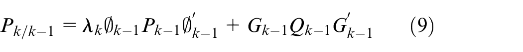
P_{k / k - 1} = λ_{k} \emptyset_{k - 1} P_{k - 1} \emptyset_{k - 1}^{'} + G_{k - 1} Q_{k - 1} G_{k - 1}^{'}

(9)

Here, the weighting factor is the forgetting factor $λ_{k}$ > 1. We see that $λ_{k}$ = 1 gives us the standard KF covariance matrix. An algorithm has been introduced to calculate the forgetting factor.^28,29 Below, we summarise the algorithm as equations (10)–(15).

Algorithm: The forgetting factor is described by equation (10) if $Q_{k}, R_{k}, P_{0}$ is positive and definite, and the matrix Hk is full-rank.²⁴

λ_{k} = \max {1, \frac{1}{n} trace [N_{k} {M^{- 1}}_{k}]}

(10)

$M_{k}$ and $N_{k}$ are obtained by equations (11) and (12), respectively.

M_{k} = H_{k} \emptyset_{k - 1} P_{k - 1} \emptyset_{k - 1}^{'} + H_{k}^{'}

(11)

N_{k} = C_{0, k} - H_{k} G_{k - 1} Q_{k - 1} G_{k - 1}^{'} H_{k}^{'} - R_{k}

(12)

The difference between the actual measurement results and the calculation with the state variables interpolated in the output vector is defined as the residual. When our model output and state estimates are exact, the residual is zero, and the optimal filter gain is achieved. To optimize the LERAFKF filter, it is essential to define the residual vector. Here, the residual vector, expressed by equation (13), exhibits characteristics of white noise.²⁹ The residual vector is defined by equation (13).

z_{k} = y_{k} - H_{k} {\hat{x}}_{k / k - 1}

(13)

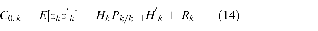
The covariance of the residuals vector is subtracted using equation (14).

C_{0, k} = E [z_{k} {z^{'}}_{k}] = H_{k} P_{k / k - 1} {H^{'}}_{k} + R_{k}

(14)

The autocovariance of the residual is:

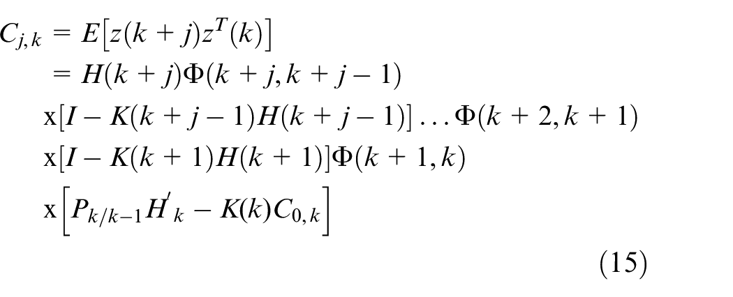
\begin{matrix} C_{j, k} = E [z (k + j) z^{T} (k)] \\ = H (k + j) Φ (k + j, k + j - 1) \\ x [I - K (k + j - 1) H (k + j - 1)] \dots Φ (k + 2, k + 1) \\ x [I - K (k + 1) H (k + 1)] Φ (k + 1, k) \\ x [P_{k / k - 1} {H^{'}}_{k} - K (k) C_{0, k}] \end{matrix}

(15)

By substituting equations (4) and (1) into equation (15), $C_{j}$ (k) is found to be zero. This confirms that the sequence of residuals is uncorrelated when the optimal gain is used.

In real-world applications, the presence of noise and imperfect parameters in our system model may cause the residual vector covariance to deviate from the specified covariance equation. Nevertheless, equation (15) is satisfied¹⁵ when the filter gain is optimally set.

P_{k / k - 1} {H^{'}}_{k} - K_{k} C_{0, k} = 0

(16)

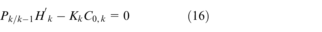
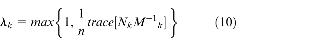
Equation (16) is satisfied when the filter gain value is optimal. This structural characteristic forms the foundation of the proposed LERAFKF filter. The data observed during the adaptation process with the fading factor is important to us, and the fading factor will be weighted based on these values. The unknown “ $C_{0, k}$ ” in equations (17)–(20) is sequentially calculated from the observed data, as follows.^17,29

C_{0, k} = D_{1, k} / D_{2, k}

(17)

D_{1, k} = D_{1, k - 1} / λ_{k - 1} + z_{k} {z^{'}}_{k}

(18)

D_{2, k} = D_{2, k - 1} / λ_{k - 1} + 1

(19)

D_{1, 0} = 0, D_{2, 0} = 0

(20)

Proof:

C_{0, k} = E [z_{k} {z^{'}}_{k}]

(21)

C_{0, k} = \frac{\sum_{i = 1}^{k - 1} σ_{i, k} z (i) z^{T} (i) + z (k) z^{T} (k)}{\sum_{i = 1}^{k - 1} σ_{i, k} + 1}

(22)

where

σ_{i, k} = Π_{j = 1}^{k - 1} \frac{1}{λ (j)}

(23)

D_{1, k} = \sum_{i = 1}^{k - 1} σ_{i, k} z (i) z^{T} (i) + z (k) z^{T} (k)

(24)

D_{2, k} = \sum_{i = 1}^{k - 1} σ_{i, k} + 1

(25)

$D_{1, k}$ and $D_{2, k}$ can be computed recursively from equations (24) to (25). This completes the proof.¹³

Simulation results

In the simulation studies, we investigated two systems, linear and nonlinear. Measurements for both systems were obtained using IMUs. For the linear system, measurements were taken from a test setup simulating a moving object. In contrast, measurements were acquired from a system modeling a missile in the nonlinear system, as shown in Figures 1 and 2, respectively.

Figure 1.

Measurement test setup for Pololu IMU01b.

Figure 2.

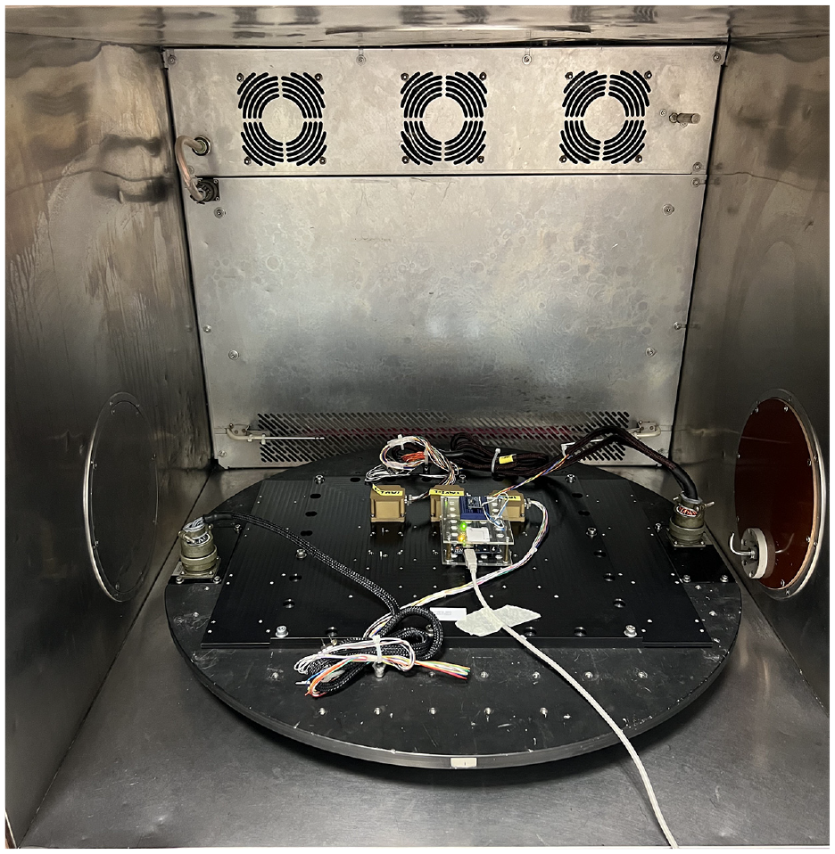
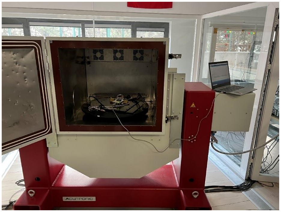
Measurement test setup for SDI33.

First, we studied a linear second-order system model similar to the one used in the study by Bar-Shalom et al.,¹⁴ representing the dynamics of a moving object. We incorporated the Pololu IMU01b model IMU into the setup for this model. Key features of the IMU include a 10-bit digital output, an accelerometer adjustable in the 2–16 g range, and a gyro output of 245–2000°/s. Equations (26) and (27) describe the moving object’s dynamics.

x_{k + 1} = [\begin{matrix} 1 & 1 \\ 0 & 1 \end{matrix}] x_{k} + [\begin{matrix} 0.5 \\ 1 \end{matrix}] w_{k}

(26)

y_{k} = [\begin{matrix} 1 & 0 \end{matrix}] x_{k} + v_{k}

(27)

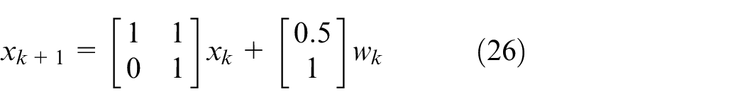
Here, the input and output disturbances are defined as a Gaussian distribution with $w_{k} ~ N (0, 1)$ and $v_{k} ~ N (0, 1)$ , respectively, for noise processes and $x_{0} = [\begin{matrix} 0 \\ 10 \end{matrix}]$ for the initial state.

We also analyzed the system described by equations (28) and (29) by slightly distorting one parameter of the system discussed in the previous paragraph. We aimed to assess and compare the performance of the KF against our proposed LERAFKF system when applied to this intentionally distorted system.

x_{k + 1} = [\begin{matrix} 1 & 1 \\ 0 & 1.1 \end{matrix}] x_{k} + [\begin{matrix} 0.5 \\ 1 \end{matrix}] w_{k}

(28)

y_{k} = [\begin{matrix} 1 & 0 \end{matrix}] x_{k} + v_{k}

(29)

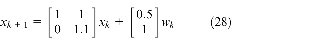
Here, the input and output disturbances are defined as in the previous paragraph.

Similarly, we tested our work with a linear and second-order system. Recognizing the importance of evaluating the effectiveness of the proposed LERAFKF filter in nonlinear and higher-order systems, we conducted tests on a three-axis rotary table in the missile measurement laboratory of the Scientific and Technological Research Council. The nonlinear system model simulating the missile is defined by fourth-order equations (equations (10) and (11)). Angular velocity values from a 9DOF SDI33 model INS, which is part of this setup placed on a three-axis rotary table, were utilized for the measurements. Key features of the INS include an accelerometer with an acceleration measurement range of up to ±20 g, 25-µg bias error, and a scale factor of less than 100 PPM; for the gyroscope, the gyro range extends up to ±550°/s, with a 0.0035°/HR bias error and less than 100 PPM scale factor.

The dynamic equations of the nonlinear system simulating the missile is described by the equation (30). Here, pitch angle is represented by $ψ$ and yaw angle is represented by $θ$ .

{\overset{\cdot}{x}}_{1} = x_{2}

{\overset{\cdot}{x}}_{2} = gcos x_{1} + gsin x_{1} - \sin 2 x_{1} - x_{2}

(30)

{\overset{\cdot}{x}}_{3} = x_{4}

{\overset{\cdot}{x}}_{4} = \cos x_{1} - x_{4}

where; $x_{1} = θ, x_{2} = \overset{\cdot}{θ}$ , $x_{3} = ψ, x_{4} = \overset{\cdot}{ψ}$ .

The nonlinear system is discretized by using “Model Discretizer” function in the Control System Toolbox available in MATLAB. First-order hold method was used for linear interpolation of inputs.

We obtained many measurements from both linear and nonlinear systems using IMUs during this study, as detailed in the previous paragraphs. The test setup configuration for the measurements is shown in Figure 3.

Figure 3.

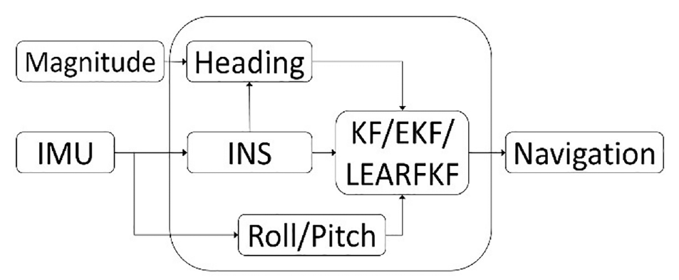
The overall test set set up configuration in block diagram form.

Extensive simulation studies were conducted using the algorithms developed in the MATLAB environment. We will summarize our simulation studies and the obtained results under three primary categories. The first study evaluated the performance of the KF when employing a linear model. The second study estimated the performance of the KF and the proposed LERAFKF when an incorrect parameter was chosen in the linear model. The third study compared the performance of the EKF and LERAFKF estimation algorithms in a nonlinear system simulating a missile.

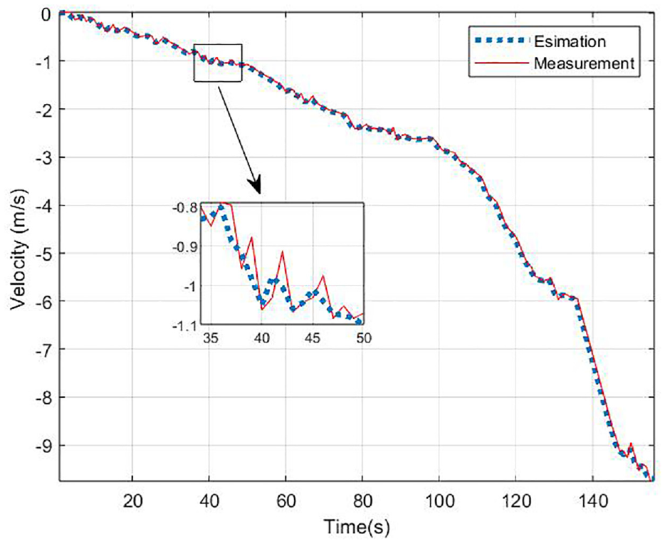
Initially, we designed the KF using a linear model to assess the accuracy of our MATLAB algorithm. The speed values obtained from processing IMU data and the speed estimated by the KF are shown in Figure 4. This figurere shows that while measured and estimated velocity values are similar, occasional deviations exist without divergence.

Figure 4.

X-axis velocity.

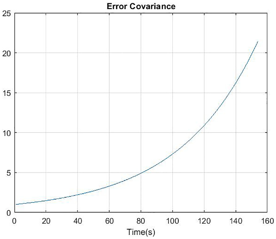
We considered the difference between predicted and measured velocity values as an error to evaluate further the consistency between the calculated velocity values derived from acceleration and the estimated velocity values. The covariance of this error shown in Figure 5 is approximately one, indicating a close match between measured and predicted velocity values.

Figure 5.

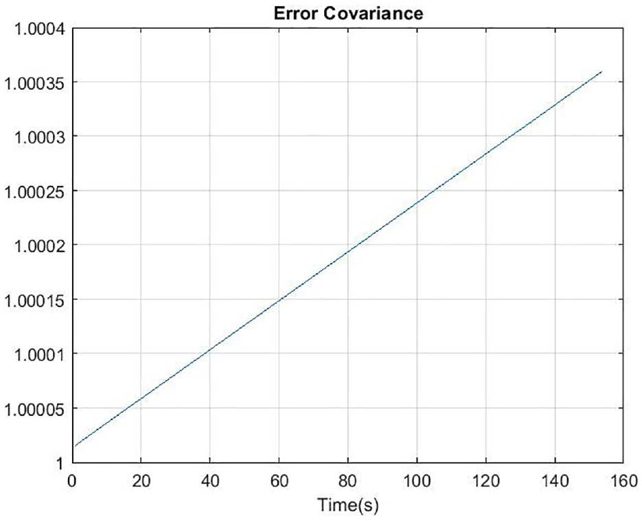
X-axis error covariance.

After validating our KF algorithm, we utilized a linear system model with imperfect parameters. Using this imperfect model, we examined the estimation performance of the KF and our proposed LERAFKF algorithm. Figure 6 shows the KF estimates of X-axis velocities compared with measurement results. As depicted in Figure 6, the estimation performance of the KF deteriorates over time, leading to convergence issues. A similar analysis for Y-axis velocity yielded comparable results, as illustrated in Figure 7.

Figure 6.

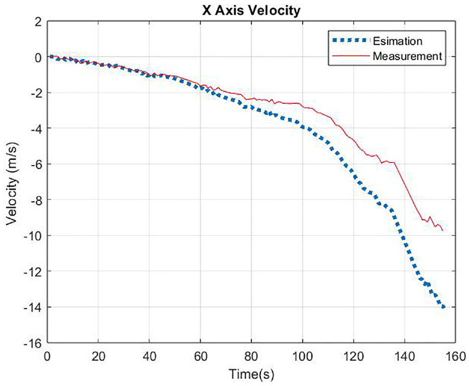
X-axis velocity (incorrect state-space model).

Figure 7.

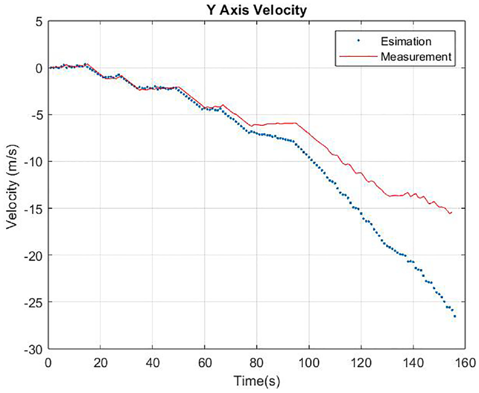
Y-axis velocity (incorrect state-space model).

The covariance value of the error is presented in Figure 8. This covariance represents the difference between estimated and measured values.

Figure 8.

X-axis error covariance (incorrect state-space model).

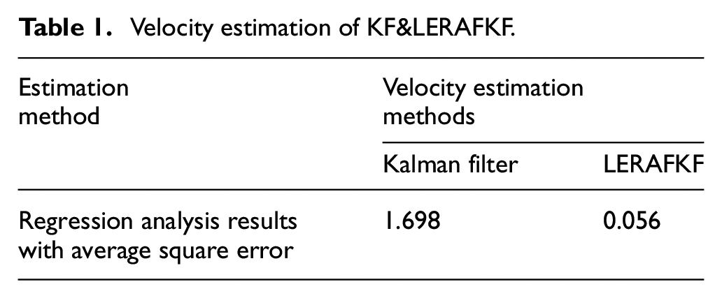
Additionally, we assessed the prediction performance of the KF and our proposed LERAFKF when an incorrect state–space is utilized. The simulation results are depicted in Figure 9. It is clear that over time, the KF estimate diverges from the measured values, whereas the LERAFKF estimates closely track the measurements. The results of regression analysis for LERAFKF and the KF’s incorrectly constructed state–space model, as defined by equations (28) and (29), are presented in Table 1. In the estimation results for different values, LERAFKF exhibits a lower mean squared error (MSE) than KF. Specifically, while the MSE for LERAFKF is approximately 0.056, the KF MSE is close to 1.698.

Figure 9.

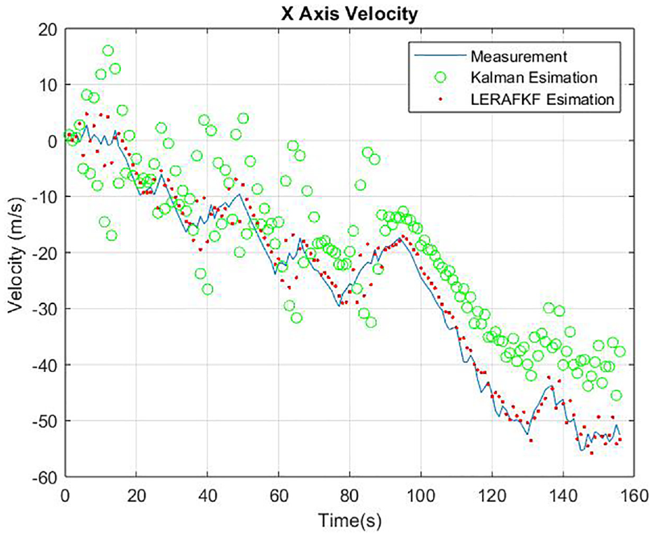
X-axis velocity (incorrect state-space model).

Table 1.

Velocity estimation of KF&LERAFKF.

Estimation method	Velocity estimation methods
	Kalman filter	LERAFKF
Regression analysis results with average square error	1.698	0.056

Lastly, we discussed the nonlinear model. Because KF is inefficient in handling this nonlinear model, we opted for the EKF. We also evaluated the performance of the LERAFKF filter in the context of the nonlinear model. The estimations of KF, EKF, and LERAFKR are plotted on the same graph given in Figure 10. From this figure, it is evident that both EKF and LERAFKF yield similar results. However, the LERAFKF demonstrates superior performance, which can be attributed to the contribution of the forgetting factor.

Figure 10.

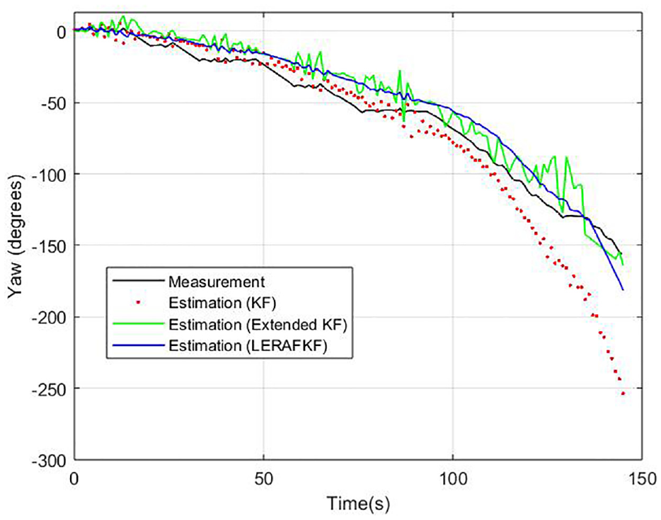
Yaw angle.

We also carried out a regression analysis for the nonlinear case. The analysis results are provided in Table 2. Here, we also see that the prediction performance of LERAFKF is better than EKF since MSE value for LERAFKF, 0.247, is smaller than the MSE value, 0.361, for KF.

Table 2.

Yaw angle estimation of EKF&LERAFKF.

Estimation method	Velocity estimation methods
	EKF	LERAFKF
Regressıon analysis results with mean square error	0.361	0.247

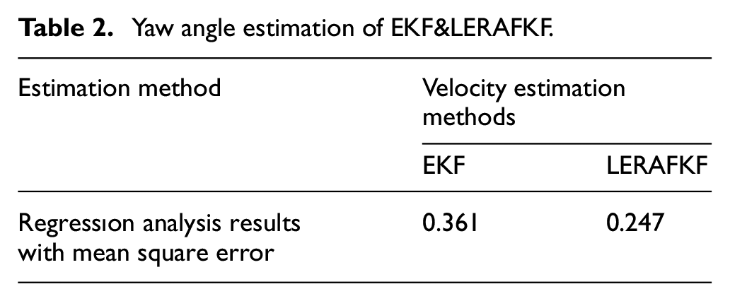
A mathematical assessment through regression analysis using the average square error method, considering the values in Tables 1 and 2, confirmed the superior prediction performance of LERAFKF.

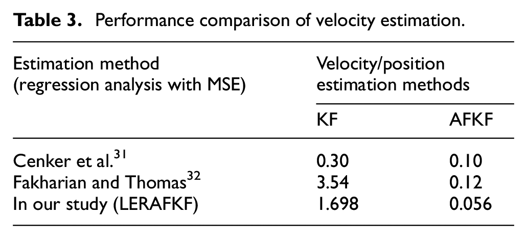
We tried to compare the performance of LERAFKF with some similar studies in the literature. The comparisons show that LERAFKF provides better prediction performance compared to these studies. In a study on speed estimation, Cenker et al.³¹ conducted a study on speed estimation. The study compared the prediction results of the Extended Kalman Filter (EKF) with their proposed “matrix adaptive damping extended Kalman filter (MAFEKF).” Another study run by Fakharian and Thomas³² compared a conventional Kalman filter with an Adaptive Kalman Filter (AKF). The results of the estimations in terms of MSE values are provided in Table 3. Here, KF stands for conventional Kalman Filter, Adaptive Kalman Filter is used for the proposed adaptive filters (MAFEKF,AKF, LERAFKF). When we compare LERAFKF performance in terms of MSE values, we see that LERAFKF performs better than these two proposed algorithms.

Table 3.

Performance comparison of velocity estimation.

Estimation method (regression analysis with MSE)	Velocity/position estimation methods
	KF	AFKF
Cenker et al.³¹	0.30	0.10
Fakharian and Thomas³²	3.54	0.12
In our study (LERAFKF)	1.698	0.056

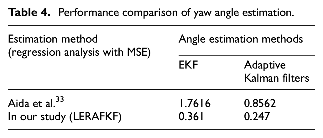
Aida et al.³³ conducted a study on Yaw angle estimation. Therefore, we found it useful to compare the results with the nonlinear system Yaw angle estimation in this manuscript. Aida etal. compared their propsed adaptive Kalman Filter with the Quaternion Kalman Filter. The results are providen in Table 4. The best result Aida et al. achieved for the MSE value in the prediction study for the Yaw angle was 1.7616 for the Quaternion Kalman filter, while it was 0.8562 for their proposed adative Kalman filter. Therefore, we can state that LERAFKF performance is better in terms of MSE values as compared to the adaptive filter proposed by Aida et al.

Table 4.

Performance comparison of yaw angle estimation.

Estimation method (regression analysis with MSE)	Angle estimation methods
	EKF	Adaptive Kalman filters
Aida et al.³³	1.7616	0.8562
In our study (LERAFKF)	0.361	0.247

Conclusion

INS take precedence in positioning systems owing to their independent operation. These systems utilize accelerometer and gyroscope sensors to measure position, orientation, and velocity. Traditionally, the KF algorithms have been employed for velocity estimation in linear systems, while EKF is utilized for nonlinear systems, where KF performance tends to be suboptimal.

In integrated GNSS–INS navigation applications, when GNSS is disabled, inaccuracies in the state–space model setup can lead to deviations in KF predictions owing to cumulative errors and measurement-related issues in the INS.

To address this issue, this study introduces a novel approach that combines the Kalman estimation algorithm with an adaptive filter featuring a fading factor. The KF is transformed into a fading factor-based adaptive Kalman filter, and the algorithm is optimized for calculating the fading factor.

In our test environment studies for linear systems, acceleration measurements were obtained using IMUs in an environment simulating a moving object. These measurements were then used for velocity estimations employing the KF and the proposed LERAFKF algorithms developed in the MATLAB environment. Additionally, a nonlinear system simulating missile motion, with a 9-degree-of-freedom XYZ system, was employed to validate LERAFKF performance. The IMU, integrated with this system, recorded acceleration and rotation measurements, which were fed into the algorithms designed in MATLAB to evaluate the estimation algorithms of both EKF and LERAFKF filters.

Detailed studies were conducted using the algorithms developed in the MATLAB environment, incorporating measurements from established test environments for both linear and nonlinear systems. The KF and EKF prediction performances were compared with that of LERAFKF. Results indicate that the proposed LERAFKF algorithm outperforms KF and EKF for linear and nonlinear systems. Notably, LERAFKF exhibits superior performance over time, whereas its prediction matches other algorithms in the initial stages.

Regression analyses confirmed the validity of the proposed algorithm. Specifically, in the context of long-term navigation applications, LERAFKF provides robust state estimates for an incorrectly constructed state–space model. However, our method does not exhibit an advantage over the KF when applied to short-term navigation applications. It is not preferred in this scenario because it imposes a heavier calculation processing load. When exploring new research avenues, one could focus on the estimation results obtained through imprecise measurement of the physical parameters of the system’s mathematical model. Utilizing system identification techniques to eliminate errors and mismatches and subsequently incorporating these outcomes into the estimation algorithm presents a promising research topic. Another area of consideration involves examining extreme conditions instead of relying solely on measurements taken at room temperature. Analyzing the sensors’ response to temperature changes and investigating the impact of inaccurate measurements on estimation results could provide valuable insights. Furthermore, more detailed studies on the interaction of LERAFKF with more complex model structures can be performed.

Footnotes

Declaration of conflicting interests

The author(s) declared no potential conflicts of interest with respect to the research, authorship, and/or publication of this article.

Funding

The author(s) received no financial support for the research, authorship, and/or publication of this article.

ORCID iD

Murat Üçüncü

Data availability statement

Data sharing not applicable to this article as no datasets were generated or analyzed during the current study.

References

Borko

Klein

Even-Tzur

. GNSS/INS fusion with virtual lever-arm measurements, Sensors (Basel) 2018; 18(7): 2228.

Angrisano

Pizzo

Gaglione

, et al. Using local redundancy to improve GNSS absolute positioning in harsh scenario. J Acta Imeko 2018; 7(2): 16–23.

Toda

Koike

. Simulation design of thermopile and magnetometer aided INS/GPS navigation system for UAV navigation. In: 8th IEEE International Symposium on Inertial Sensors and Systems, 22–25 March 2021, INERTIAL 2021 - Virtual, Kailua-Kona, p. 1. USA: Institute of Electrical and Electronics Engineers Inc.

Titterton

Weston

. Progress in Astronautics and Aeronautics Series. 2nd ed. 2021. AIAA.

Gao

Yongmin

, et al. Cubature Kalman filter with both adaptability and robustness for tightly-coupled GNSS/INS integration. J IEEE Sens 2021; 21(13): 14997–15011.

Song

Kim

, et al. Performance enhancement and countermeasure for GPS failure of GPS/INS navigation system of UAV through integration of 3D magnetic vector. J Posit Navigat Timing Perform 2018; 7(3): 155–163.

Tan

Wang

Zhu

, et al. Improved alignment method for a SINS using two vector measurements. In: Proceedings of the 5th International conference on instrumentation and measurement, computer, communication and control (IMCCC), Qinhuangdao, China, 18–20 September 2015, pp. 1674–1678. IEEE.

Xile

Haiyong

Bokun

, et al. RL-AKF: an adaptive Kalman filter navigation algorithm based on reinforcement learning for ground vehicles. J Remote Sens 2020; 12; 35(1): 416–425.

Zhang

Wang

Neusyoina

, et al. New adaptive Kalman filter for navigation systems of carrier-based aircraft. Chin J Aeronaut 2021: 1704.

10.

Kalman

. A new approach to linear filtering and prediction problems. J Basic Eng 1960; 82: 35–45.

11.

Mehra

. Identification of stochastic linear dynamic systems using Kalman filter representation. J AIAA 1971; 9(1): 2828.

12.

Lee

. Theory and application of adaptive fading memory Kalman filters. J IEEE Transact Circuits Syst 1988; 35(4): 474–477.

13.

Xia

Shen

. Adaptive fading Kalman filter with an applications. J Automat 1994; 30: 1333–1338.

14.

Bar-Shalom

Kirubarajan

. Estimation with applications to tracking and navigation. J Comput Sci, Epub ahead of print 4 January 2002. DOI:10.1002/0471221279.

15.

Hide

Moore

Smith

. Adaptive Kalman filtering for low-cost INS/GPS. J Navigat 2003; 56: 143–152.

16.

El-Sheimy

Hou

Niu

. Analysis and modeling of inertial sensors using Allan variance. J IEEE Trans Instrum Meas 2008; 57: 140–149.

17.

Ding

Wang

Rixos

, et al. Improving adaptive Kalman estimation in GPS/INS integration. J Navigat 2007; 60: 517–529.

18.

Ngoc

Khenchaf

Comblet

. Evaluating process and measurement noise in extended Kalman filter for GNSS position accuracy. In: Proceedings of the 13th European conference antennas propagation, EuCAP, Krakow, Poland, 31 March–05 April 2019. IEEE.

19.

Faragher

. Understanding the basis of the Kalman filter via a simple and intuitive derivation. IEEE Signal Process Mag 2012; 29: 128–132.

20.

Bou

Zhenwei

Shicai

, et al. Integrated navigation algorithm based on multiple fading factors Kalman filter. Sensors (Basel) 2022; 22: 5081.

21.

Kai Wei

Cheng An

Kun Yao

. The performance analysis of an AKF based tightly-coupled INS/GNSS sensor fusion scheme with non-holonomic constraints for land vehicular applications. J Appl Mech Mater 2013; 284–287: 1956–1960.

22.

Takaki

Nobuaki

. Performance assessment of adaptive Kalman filter-based GNSS PVT and integrity in dense urban environment. J Trans Navigat 2019; 4: 49–58.

23.

Ozbek

Babacan

Efe

. Stochastic stability of the discrete-time constrained extended Kalman filter. Turk J Electrical Eng Comp Sci 2010; 18: 211–223.

24.

Zarchan

Musoff

. Fundamentals of Kalman filtering: a practical approach. 4th ed. 2013. USA: American Institute of Aeronautics and Astronautics.

25.

Hashlamon

Erbatur

. An improved real-time adaptive Kalman filter with recursive noise covariance updating rules. Turk J Electrical Eng Comp Sci 2006; 24: Article 14.

26.

Ozbek

Efe

. Fading Kalman filter for maneuvering target tracking. J Turk Stat Assoc 1999; 2: 193–206.

27.

Orderud

Sælands

. Comparison of Kalman filter estimation approaches for state space models with nonlinear measurements. J Eng Math 2005; 7(9): 1–8.

28.

Peng

Zhongliang

Liangbin

. Adaptive fading factor unscented Kalman filter with application to target tracking. J Aerosp Syst 2021; 4: 1–6.

29.

Kim

Jee

Park

, et al. The stability analysis of the adaptive fading extended Kalman filter using the innovation covariance. Int J Control Automat Syst 2009; 7: 49–56.

30.

Won

Daehee

Jongsun

, et al. Performance improvement of inertial navigation system by using magnetometer with vehicle dynamic constraints. J Sens 2015; (1): 1–11.

31.

Cenker

Esin Köksal

Levent

. Stability of the adaptive fading extended Kalman filter with the matrix forgetting factor. Turk J Electrical Eng Comp Sci 2012; 20: Article 11.

32.

Fakharian

Thomas

. Adaptive adjustment of noise covariance in Kalman filter for dynamic state estimation. In: 011 International Conference on Networking, Sensing and Control, ICNSC, Delft, Netherlands, 11–13 April 2011, pp. 181–185. IEEE.

33.

Aida

Hassen

Alain

. Energy-aware adaptive attitude estimation under external acceleration for pedestrian navigation. IEEE/ASME Trans Mechatron 2016; 21: 1366–1375.

Improving the performance of a MEMS-IMU system based on a false state-space model by using a fading factor adaptive Kalman filter

Abstract

Keywords

Introduction

Kalman filter and extended Kalman filter estimation algorithm

Adaptation of Kalman filter with low error rate fading factor

Simulation results

Conclusion

Footnotes

Declaration of conflicting interests

Funding

ORCID iD

Data availability statement

References