
Abstract
Arimatsu Narumi Shibori (thread-tying), which is a traditional craft, has a history of more than 400 years and has been handed down to artisans in Japan. Recently, the shortage of successors to artisans has emphasized the maintenance of this thread-tying technique. To achieve this, Arimatsu Narumi Shibori needs to be elucidated based on scientific knowledge using numerical analysis techniques, which has not been achieved so far. In this technique, the fabric is complexly deformed, and complex wrinkles are formed in it. One possible approach for modeling this fabric is the use of a shell element that does not have an element volume. As the tensile and bending stiffnesses of the shell element are evaluated using a single Young’s modulus, the bending stiffness increases with the tensile stiffness. Therefore, unlike the deformation achieved by the actual fabric-tying, this fabric analysis model cannot achieve large deformation of the fabric. In this study, a tying analysis method is proposed to elucidate Arimatsu Narumi Shibori. In this method, the fabric is modeled using three layers of shell elements to reproduce the fabric behavior. The material properties of the three-layer structure are presented based on the tensile test, the bending test and the friction test. Using the proposed method, we could visualize the stress distribution and wrinkles in the fabric-tying and elucidate its breaking condition.
Keywords
Introduction
Arimatsu Narumi Shibori
Arimatsu Narumi Shibori is a tie-dye produced mainly in the Arimatsu Narumi area of Nagoya City,1–4 which is officially designated as the first traditional craft in Aichi Prefecture, Japan. An example of this craft is shown in Figure 1. The dyed pattern by the Arimatsu Narumi Shibori Robot is shown in the Figure 2. The tie-dye technique has been handed down for approximately 400 years and, since then, has maintained high quality. There are various patterns available based on the different techniques used. However, the future of Arimatsu Narumi Shibori is in jeopardy due to the aging of artisans and the difficulty faced in finding successors. Currently, these crafts are mainly produced overseas, with domestic production continuously declining.
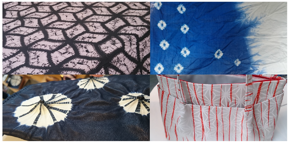
Pattern of Arimatsu Narumi Shibori (Arimatsu Narumi tie-dye).
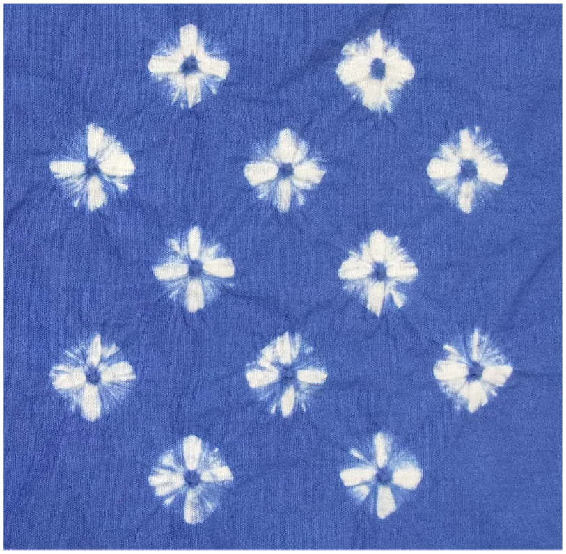
Dyed pattern by the Arimatsu Narumi Shibori Robot.
Traditional tying and indigo dyeing
The most important and difficult task in producing Arimatsu Narumi Shibori is thread-tying. The traditional thread-tying and tie-dyeing processes are shown in Figure 3, and the indigo-dyeing patterns obtained in the tie-dyeing process are shown in Figure 4. Dye penetration into the tightened fabric is prevented using the resist dyeing method. In contrast, the dye penetrates the nontightened fabric. When the thread is removed from the fabric after dyeing, a complex pattern is formed through the composition of both the dye area and the resist dye area. A variety of artisanship is required for tie dyeing, where each task has to be performed manually. Therefore, many people need to be hired for mass production.
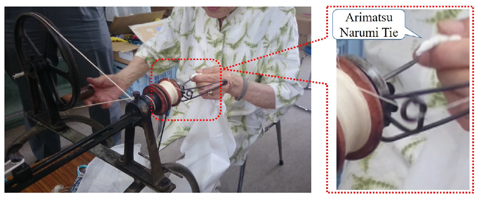
Traditional thread-tying task performed by artisans in the Arimatsu-Narumi region.
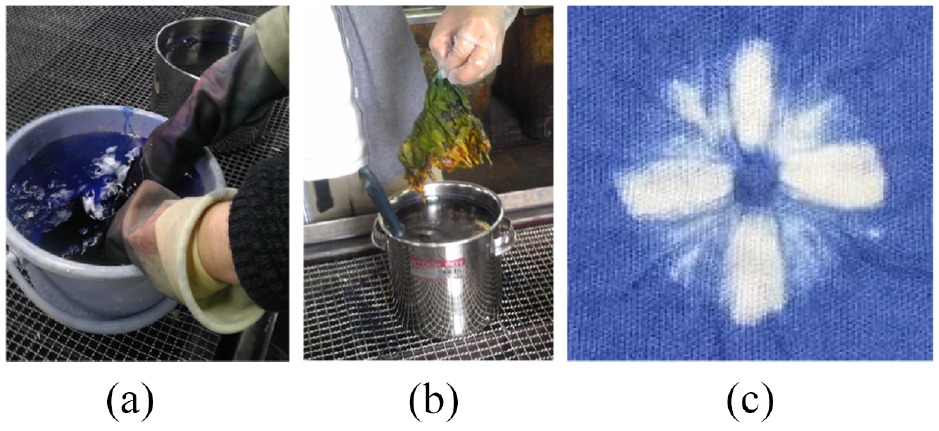
Traditional dying work of fabric in Arimatsu Narumi region (immediately after the fabric is taken out, the dye on it turns green and turns blue over time): (a) dying of fabric, (b) taking out fabric from dye, and (c) front view of fabric.
Arimatsu Narumi Shibori Robot implemented by cap tie dye
Various machines are available that assist in the tie-dyeing process; however, they are yet to be fully automated and are largely dependent on artisans’ skills. Thus, to increase productivity and reduce costs, alternative mechanical systems are required. The tie-dyeing mechanization with a flexible fabric requires technology to fix the fabric and perform thread-tying of the fabric. We have previously prototyped a tie-dyeing robot by using a multistage cylinder as a tying tool.
5
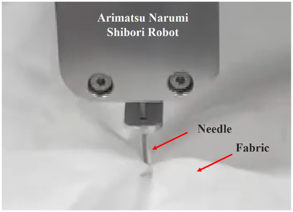
In the tying process, a metal rod is inserted into the multistage cylinder, which is formed of silicone rubber. A fabric is sandwiched between the cylinder and metal rod and then pushed into the cylinder. In this paper, this multistage cylinder is called the cap, and the metal rod is called the needle. After pulling the needle back to the initial position, the fabric is tightened inside the tube of the cap, as shown in Figure 6 and then immersed in the dye while maintaining the cap-tying state. Figure 5 shows the thread-tying performed by artisans and cap-tying performed by a robot. A cap-tying is proposed to simplify the traditional tie, for the robots to operate.
5
Figure 6 shows the cap structure and cap-tying process, which replaces the traditional thread-tying process. The cap is cylindrical, with a height
Tie (Shibori): (a) traditional thread tying (Kumo shibori) by Arimatsu-Narumi artisans and (b) cap tying by Arimatsu-Narumi Shibori robot.
Structure of the cap: (a) cross section of cap and (b) cross section of cap attached to fabric.
Structure of Arimatsu Narumi Shibori Robot
Figures 7 and 8 show an overall view of the robot that attaches the cap to the fabric. The International Automation Industry (IAI)’s linear actuator RCP5-SA4C is applied to move the needle up and down. To continuously attach the cap to the fabric, cartridges are mounted in the robot, which can be located using multiple caps. After mounting each cap, the IAI rotary actuator RCP-RTCSL is applied to rotate the cartridge.
Photograph of Arimatsu Narumi Shibori robot.
Structure of Arimatsu Narumi Shibori robot.
Movement of Arimatsu Narumi Shibori Robot
Figure 9 shows a series of operations performed for attaching the cap to the fabric. The parameter
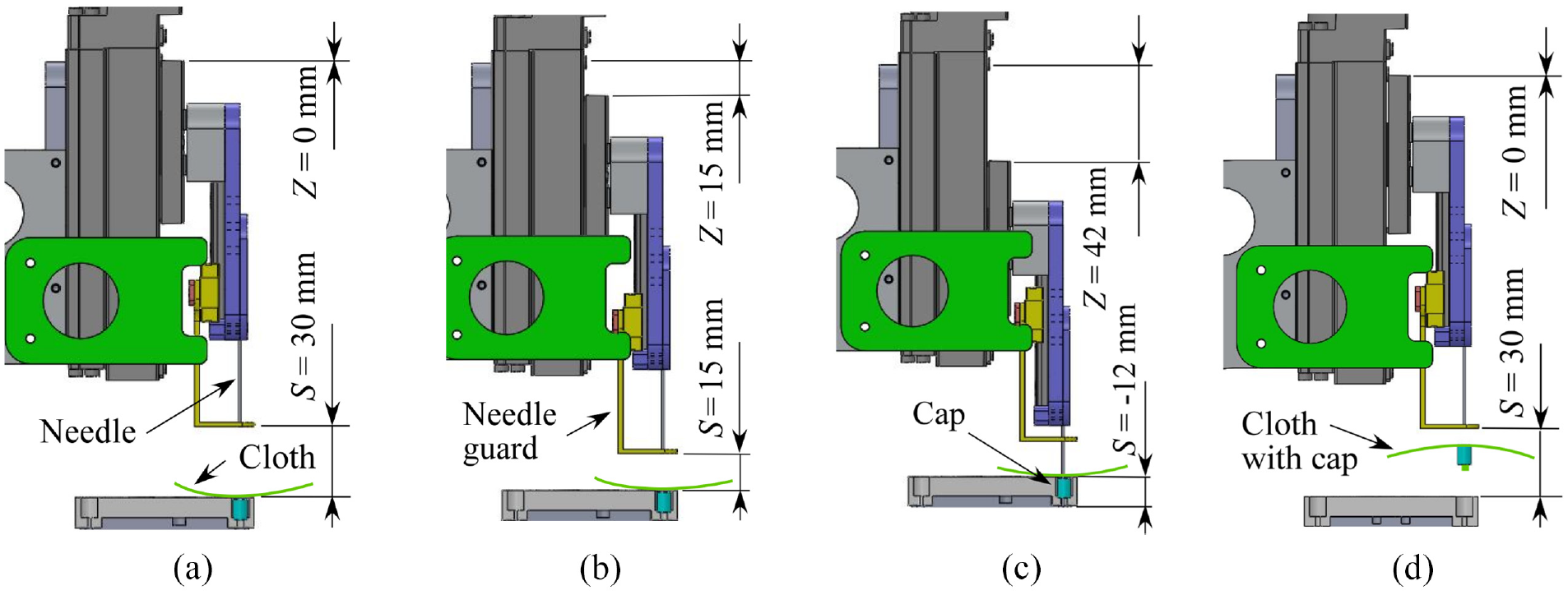
Movement of Arimatsu Narumi Shibori robot during fabric tying operations: (a) wait, (b) vertical descent, (c) mounting, and (d) separation.
FEM modeling of fabric
The study of fabric modeling began in the 1930s. 6 The finite element method was used to analyze the fabric behavior during the 1990s. Fabric deformation was characterized by large displacements and rotations, whereas the small strains were analyzed using a geometric nonlinear finite element method. 7 The nonlinear material response was measured using the Kawabata bending test system. Fabric contact with rigid surfaces was used to develop a simulated 3D motion that is related to the actual fabric manufacturing process. 8 By implementing the ANSYS/LS-DYNA software, the penetration of a knife through a plain-woven fabric was simulated to improve the process of stabbing and the mechanism of fiber breakage. 9 The mechanical behavior of the woven fabric under compression was investigated using 3D finite element analysis in conjunction with a nonlinear mechanical model for the yarn. 10 A general approach to simulate the mechanical behavior of textile materials is presented. This approach, formulated in a large displacement and finite strain framework, was based on the representation of all fibers constituting the woven structures by means of 3D beam models and on the consideration that there exists contact-friction interaction between fibers. 11 To achieve the hybrid element analysis (HEA) approach, multi-scale fabric modeling (yarn to fabric) was realized using the LS-DYNA and finite element formulations. 12 To model a fabric that can predict the relationship between the stress mechanical properties and structural parameters, the stress predicted by the finite element model was validated against the experimental results. 13 An efficient numerical technique to automatically construct and simulate a fabric assembly for mechanical predictions was developed using the TexGen and ABAQUS. The modeling technique was evaluated and validated using a standard fabric testing system, the Kawabata evaluation system. 14 To improve the modeling of the bending behavior of plain-woven fabric, the physical and mechanical parameters of the fabric samples were measured using the Kawabata Evaluation System for Fabric(KES-F). 15 The modeling of the woven fabric textiles was demonstrated under in-plane shear loading. The behavior of textiles under shear load was examined and verified using a combination of TexGen and ABAQUS software. 16 The tensile behavior of the nonwoven fabric at the macroscale was studied using ABAQUS. The laminate orientation was considered with the orientation distribution function, which was obtained by analyzing the data acquired from scanning electron microscopy with Hough transform methods. 17 The woven microgeometry of the 3D woven fabric was obtained using the virtual fibers consisting of chains of truss elements. 18 A nonlinear hypoelastic discrete model was developed for the materials with two orthogonal directions of strong anisotropy. The experimental characterization provided the numerical data to produce a representational prediction of the deformed fabric geometry and shear angle distribution. 19 The bias-extension test was simulated using different approaches and the material models with the numerical finite element code LS-DYNA. The material model MAT MICROMECHANICS DRT FABRIC was the best suited to capture the load-displacement trend of the experimental bias-extension test. 20 To estimate the shear modulus of a continuous yarn model for FE modeling of ballistic impact events, a reverse engineering method was presented for continuous yarn models of different materials. 21 The bursting behavior of the spun-bonded nonwovens with different MPUAs was simulated based on the damage and the layered structure using the FEM. 22 In the literature, any models of fabric tying have not been proposed or analyzed for fabric tying modeling.
Purpose
In the thread-tying process performed by artisans, the fabric is subjected to compressive stress rather than tensile stress. As shown in Figure 9(a), in the cap-tying performed by the Shibori robot, the fabric is placed on the hollow cylindrical cap and pushed inside by the cylindrical needle. This generates frictional forces between the fabric and the cap or between the fabric and the needle. Under this force, tensile stress is generated locally or transiently on the fabric. As shown in Figure 10(a), as the needle load decreases, the fabric does not protrude from the cap tip. Therefore, the dye pattern cannot be formed on the fabric. As shown in Figure 10(b), the fabric breaks if the load on the needle exceeds the threshold value. Thus, to stably tie the fabric into the cap, an appropriate material and a design need to be obtained for the cap. In this study, to predict the tying behavior, which affects the dye pattern of Arimatsu Narumi Shibori, we propose, for the first time, a tying modeling method. This tying modeling method is based on finite-element modeling analysis using LS-DYNA, which predicts the stress distribution on the fabric.23,24
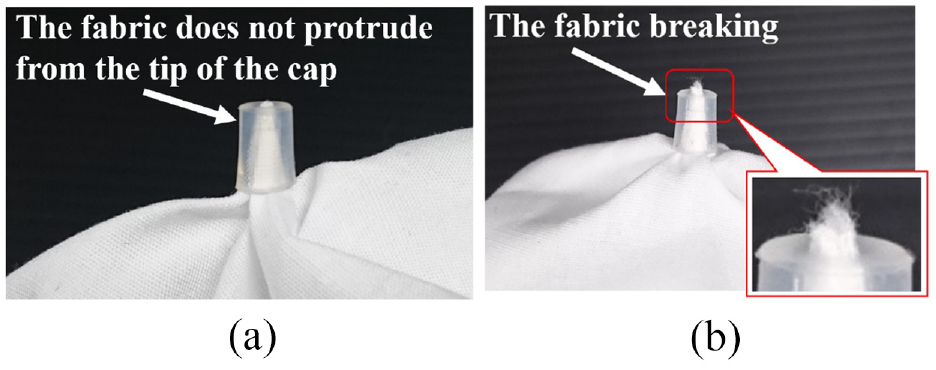
Cap-tying by Arimatsu Narumi Shibori robot: (a) case of excessive load on needle and (b) case of insufficient pushing of needle.
Stiffness evaluation of Arimatsu Narumi fabric
Fabric tensile test
To investigate the characteristics of the fabric used for Arimatsu Narumi-tying, the fabric is subjected to a tensile test. The fabric has dimensions of 290 mm × 290 mm, and its thickness and density are approximately 0.17 mm and
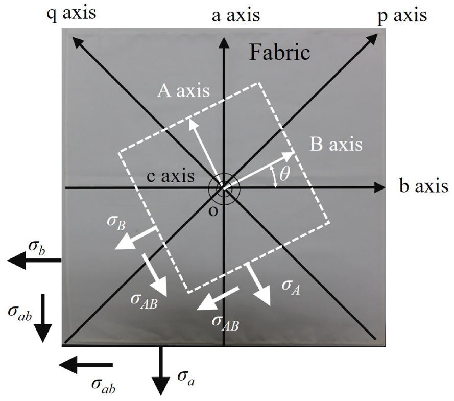
Coordinate axes on the fabric (directions of the warp threads and weft threads are defined as the a- and b-axis directions, respectively.).
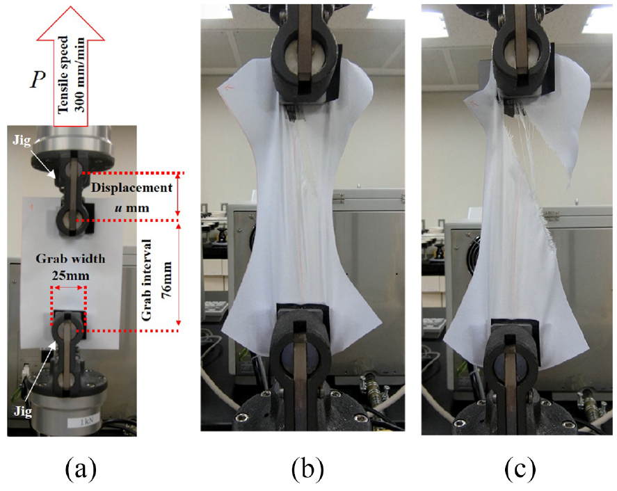
Tensile test performed using the grab method: (a) time step 1 (initial condition), (b) time step 2 (tensile test with respect to q-axis), and (c) time step 3 (fabric breaking) (tensile test with respect to q-axis).
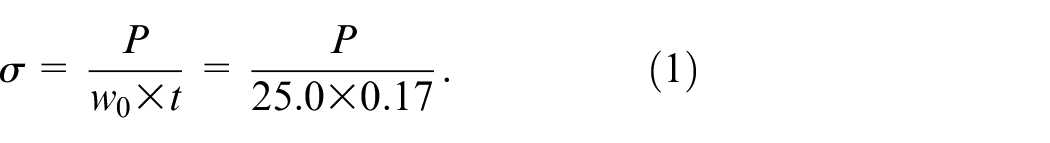
Figure 13 presents the load-displacement curve, where the load
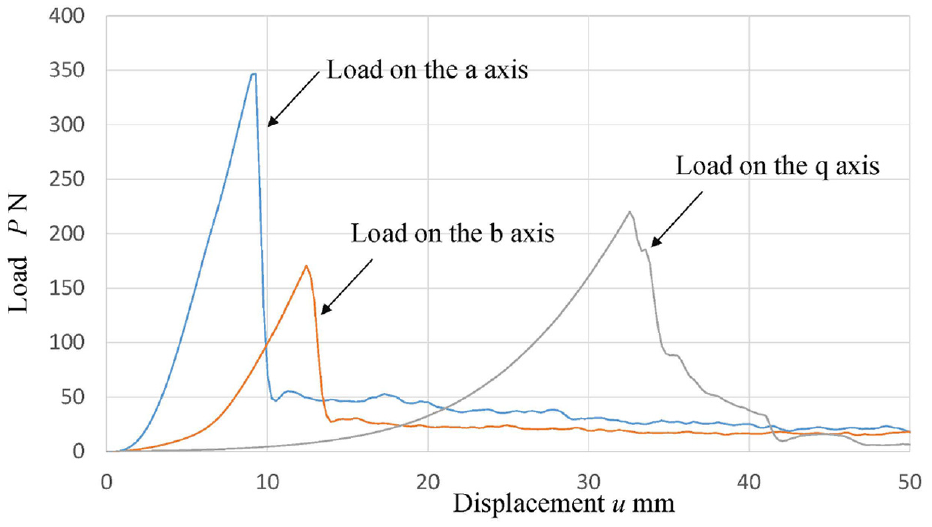
Load-displacement diagram of Arimatsu Narumi fabric (Model number: # 19300 40) manufactured by Sunwell Co., Ltd.
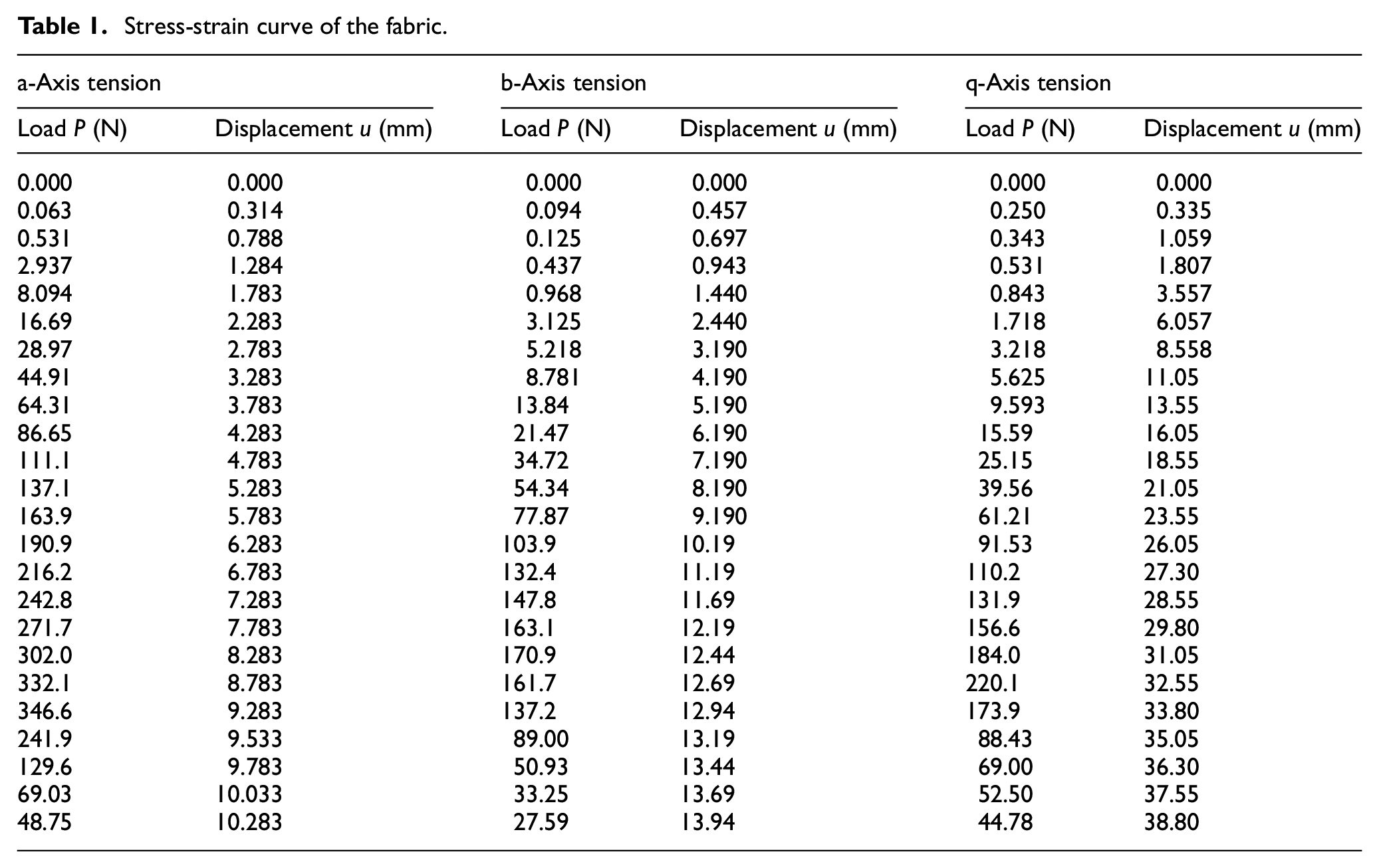
Stress-strain curve of the fabric.
The grab interval is 76 mm. Let
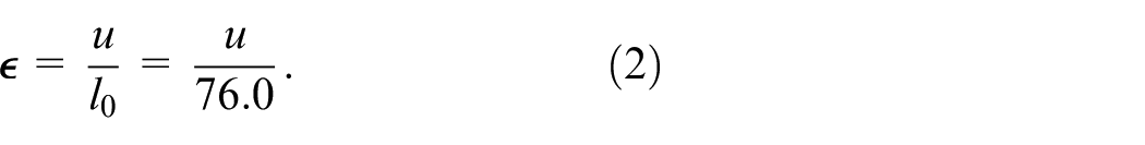
By using the data obtained from these conversion formulas, both LS-DYNA commands * MAT_FABRIC and * DEFINE_CURVE are set. 24
Fabric-bending test
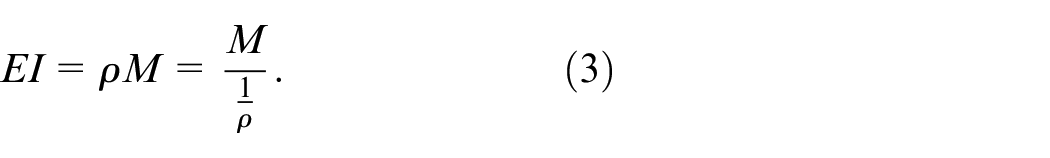
As the fabric causes a complicated large deformation, including wrinkles, the shell element should be applied during finite-element modeling (FEM) of the fabric. As a solid element with volume is applied to the fabric modeling, the mesh elements are turned inside-out because of a large deformation. The negative volumes cause numerical divergence, and the calculation cannot be completed. However, as the shell elements do not have volume, they can be robustly completed for calculations performed for even large deformations. In contrast, if a shell element is applied to the fabric modeling, the bending stiffness problem is incurred. The tensile stiffness of the fabric is not equal to its bending stiffness. It takes considerable effort to tear the fabric, however the fabric can be easily folded. The bending stiffness is independent of the tensile stiffness; therefore, it is necessary to evaluate the bending stiffness of the fabric using a bending tester. The bending stiffness of the fabric can be expressed as29,30
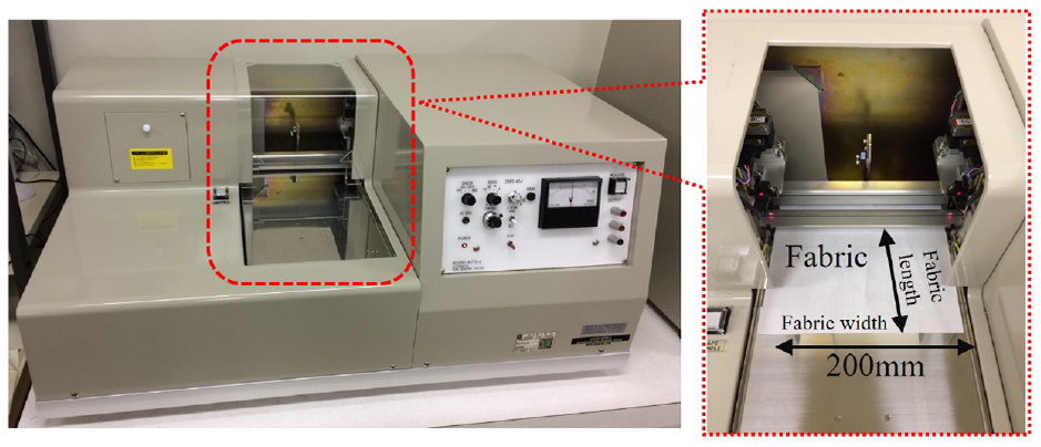
The bending moment − curvature graph can be obtained using a bending tester manufactured by Kato Tech (model number: KES-FB2-A),31–34 as shown in Figure 14. The parameters
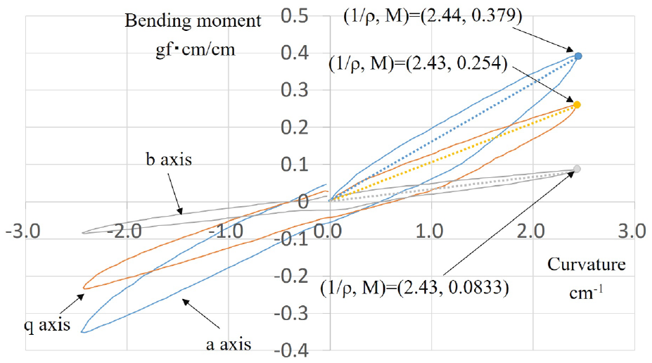
Bending characteristics of the fabric (The horizontal axis represents the reciprocal of the curvature
As LS-DYNA is not implemented for a stable analysis that accounts for this hysteresis, the curve of Figure 15 is approximated by a single straight line to evaluate the bending stiffness. As shown in Figure 15, the maximum bending moments
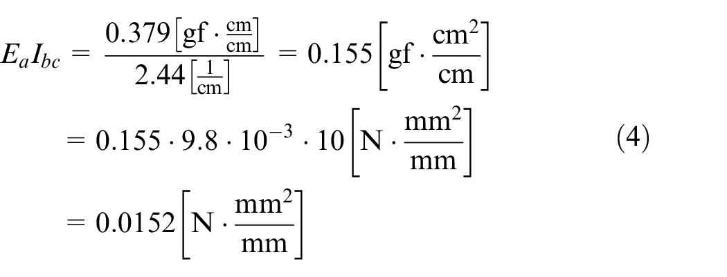
The above value shows the bending stiffness per millimeter of the fabric width. As shown in Figure 14, the fabric width is 200 mm. The bending stiffness (unit: N·mm 2) can be obtained by multiplying the above value by 200 mm. The variable


The variable
Tensile test of silicone rubber (cap) and LS-DYNA implementation
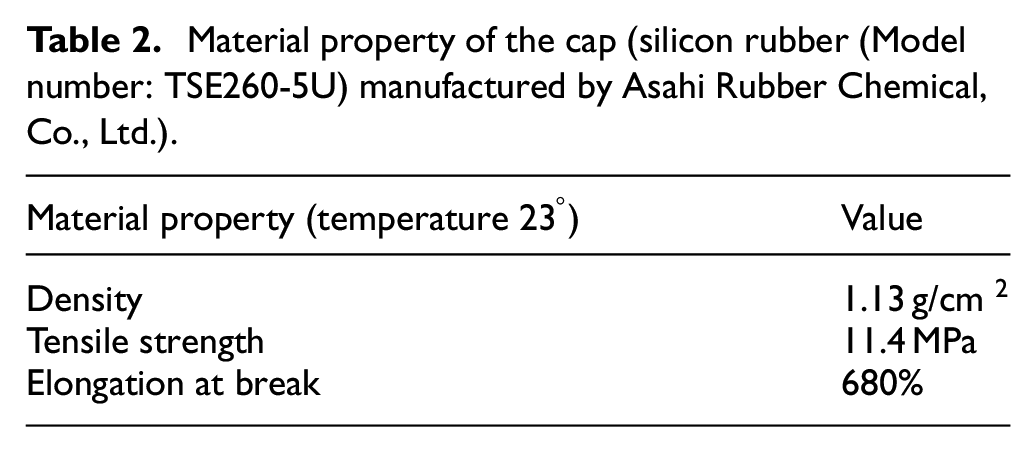
The cap is applied to tighten the fabric, whose tying part is immersed in the dye. The dye penetration is suppressed by the cap tightness, which is formed by elastic silicone rubber. This silicone rubber is manufactured by Asahi Rubber Chemical, Co., Ltd. (model number TSE260–5U), and the material properties are summarized in Table 2. To obtain the stress-strain curve of silicone rubber, the test is conducted using the tensile tester (model number: AG-50kNXplu36,37) manufactured by Shimadzu Corporation. As shown in Figure 16(a), a dumbbell shape (JIS K 6251 dumbbell shape No. 3
38
) is produced. Figure 16(b) to (d) shows the time history of the tensile test. Two black points are marked on the dumbbell shape. Through image processing, the strain is calculated from the moving distances of the two points. The stress-strain curve is shown in Figure 17. The dumbbell stretches to approximately seven times its initial length and is then cut by the load. Transient stress concentration may occur in the tying analysis performed by FEM. The material properties of the cap are listed in Table 2. If an instantaneous stress of 10 MPa is generated due to the stress concentration, approximately 800% strain is induced on the cap. The strain is defined as
Material property of the cap (silicon rubber (Model number: TSE260-5U) manufactured by Asahi Rubber Chemical, Co., Ltd.).
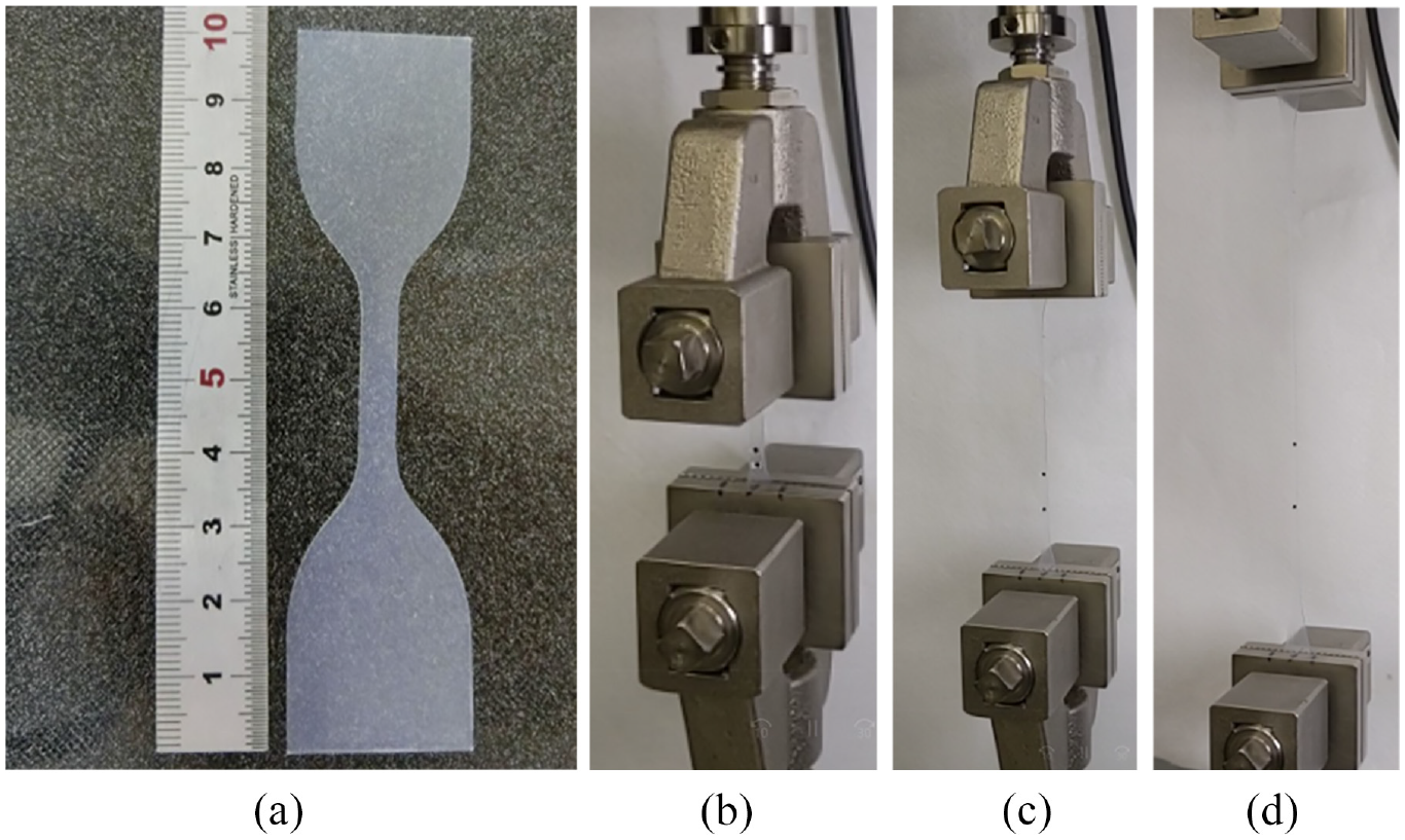
Tensile test of silicone rubber: (a) time step 1 (Initial condition: Dumbbell shape made of silicone rubber), (b) time step 2, (c) time step 3, and (d) time step 4.
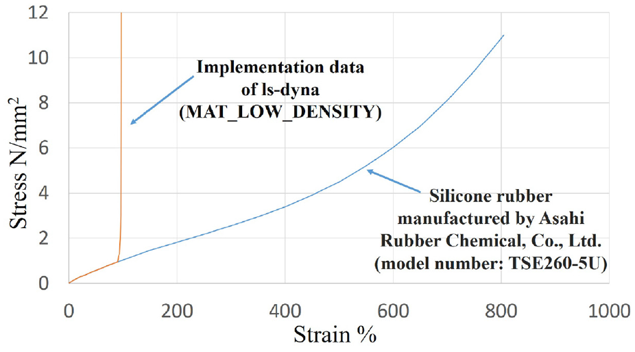
Stress-strain curve of silicone rubber (cap).
Friction
Friction test method and tester
In the tying task of the robot, the fabric is pulled into the cap by using a needle, and friction is generated between the fabric and cap. The needle is pushed in until the fabric sticks out of the cap. Then, with the fabric fixed on the cap through friction, only the needle is pulled back to the initial position. Therefore, the friction coefficient between the fabric and cap must be larger than that between the needle (steel) and fabric.
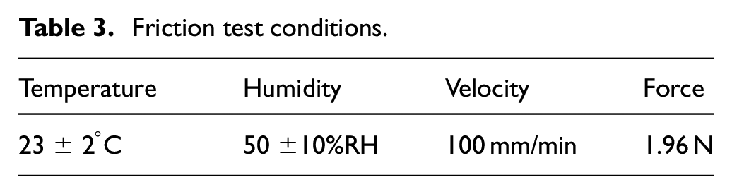
These friction evaluations are conducted and applied to the finite-element model of the tying. Three types of friction are generated in the friction test: friction between the silicon (the cap) and fabric, friction between the needle (steel) and fabric, and friction between two pieces of the fabric. The friction tests are performed based on JIS K7125. 39 Figure 18 shows the state of the friction test, where INSTRON 5566 is used as the testing machine40–42; the friction test conditions are summarized in Table 3.
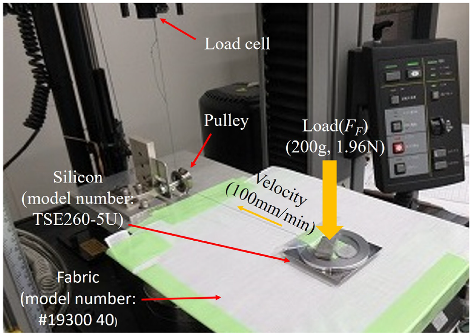
Measurement of friction coefficient between the fabric and silicon based on the friction test method, JIS K 7125 (see friction test conditions in Table 3).
Friction test conditions.
Results of friction test
A spring is connected to the load cell, which in turn is connected to the test piece through a pulley. By moving the load cell, the silicon test piece slides on the fabric, as shown in Figure 18. At this time, the slipped displacement and load are measured. As shown in Figure 19, the horizontal and vertical axes represent the displacement (mm) and load (kgf), respectively. The logarithm is taken for the displacement on the horizontal axis.
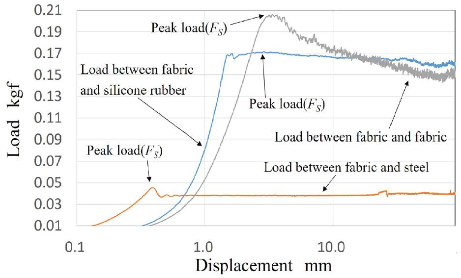
Semilog displacement plot between load (kgf) and displacement (mm).
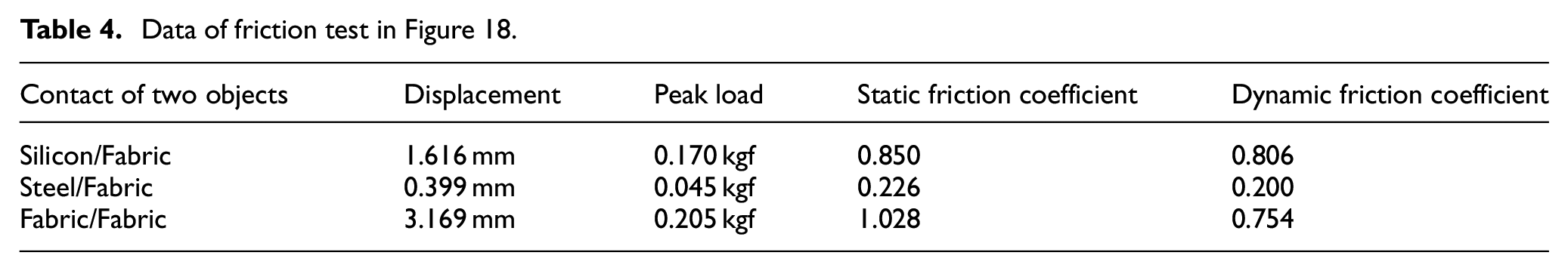
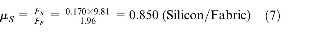
The results obtained using the graph are summarized in Table 4. As the load cell moves, the measured load increases linearly, because the sample (silicon in Figure 18) is pressed by an object mass on the fabric. Furthermore, the load induced by the spring increases as the load cell moves. Eventually, this load exceeds the frictional force. The test pieces (silicon in Figure 18) start sliding on the sample (fabric in Figure 18). The coefficient of static friction (silicon/fabric) is obtained as follows:
Data of friction test in Figure 18.
Here,
The calculation example of the above formula is the dynamic friction coefficient between the silicone rubber and fabric, as shown in Table 4.
FEM model of fabric
LS-DYNA implementation based on fabric tensile test
LS-DYNA (keyword *MAT_FABRIC) is applied to the fabric model. The membrane formulation for fabric material is applied to FORM=14.
24
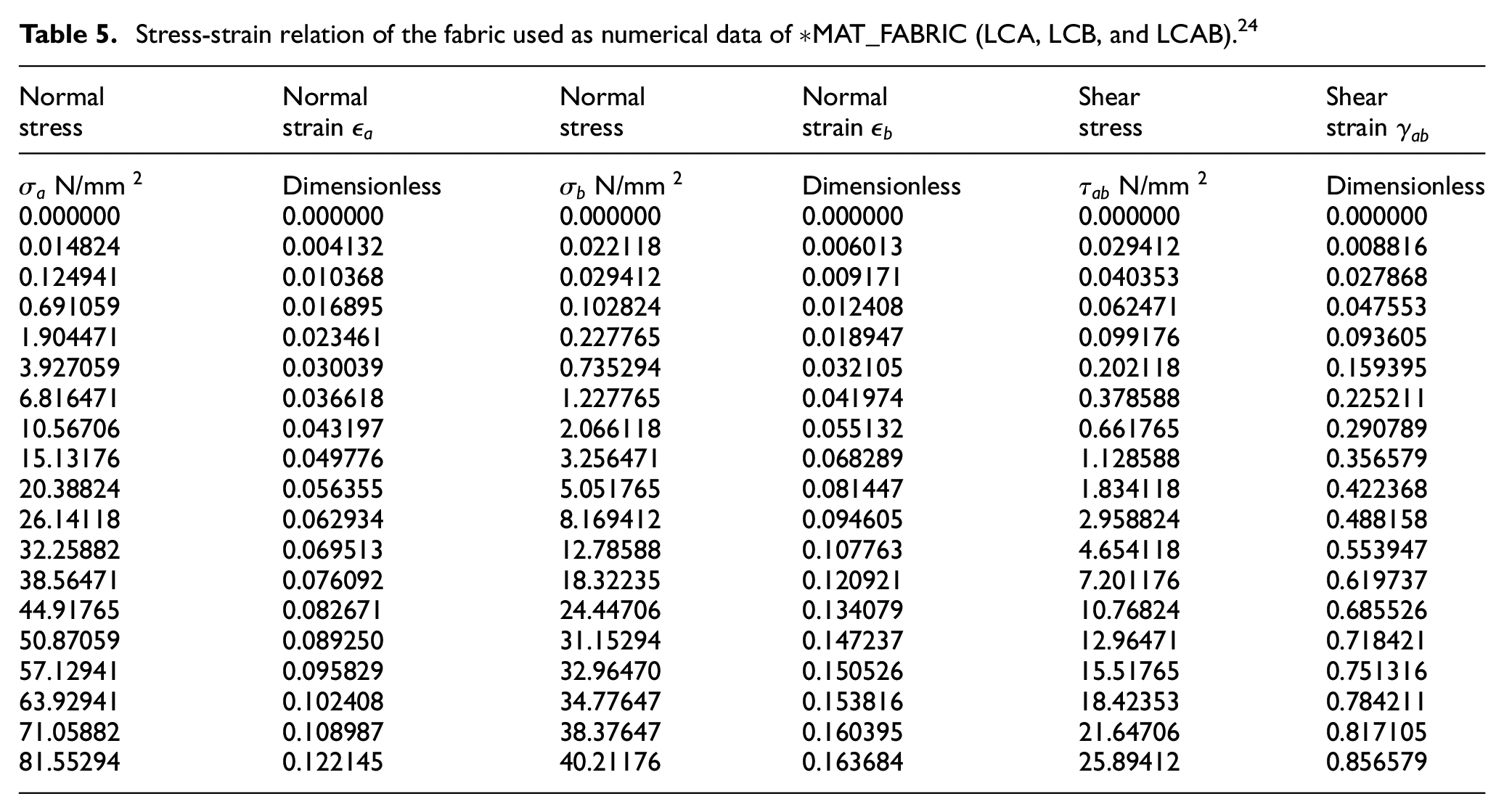
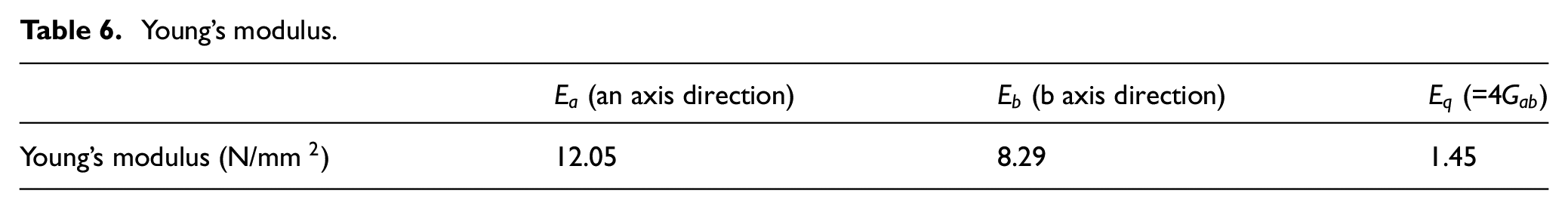
The data used in the LS-DYNA keyword file are summarized in Table 5, and the analysis results of this paper can be reproduced. Based on the numerical data presented in Table 1, the strain and stress are calculated using equations (1), (2), (A.11), and (A.12). The Young’s moduli
Stress-strain relation of the fabric used as numerical data of *MAT_FABRIC (LCA, LCB, and LCAB). 24
Young’s modulus.
LS-DYNA implementation based on fabric-bending test
As mentioned in Section 3.2, shell elements are applied in the fabric modeling. If stiffness based on the tensile test is applied as the stiffness of the shell element, the bending of the shell element stiffness increases beyond the expected value. The stiffness of this shell element affects both tensile stiffness and bending stiffness. In contrast, if the membrane element is applied as the fabric model, bending stiffness does not occur on the fabric model. The analysis behavior of the shell element differs from the original behavior of the fabric. Nishi et al. proposed a macroscale model that can analyze the out-plane bending stiffness independently of the in-plane tensile stiffness on the fabric plane.35,46 The structure of the fabric model is shown in Figure 20, which is a sandwich structure comprising a shell element, a membrane element, and a shell element. The material setting for the LS-DYNA keyword, *MAT_ORTHOTROPIC_ELASTIC, 24 is applied to the shell element, and *MAT_FABRIC 24 is applied to the membrane element.
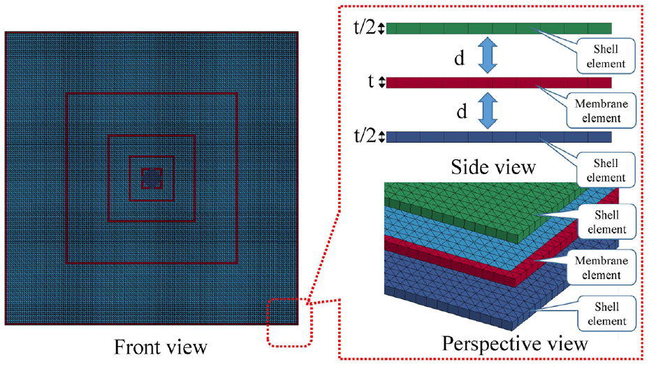
FEM model of the fabric.
The membrane element is placed in the center of the thickness direction, whereas the shell elements are placed at both ends of the thickness direction. The nodes of the shell element are shared with those of the membrane element. The in-plane tensile stiffness is analyzed using the membrane element, and the out-plane bending stiffness is analyzed using the shell element. The center of the membrane element thickness is defined as the origin. The two shell elements on both sides are located equidistant from the center of the membrane element thickness. Let
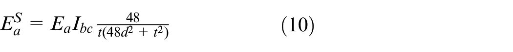
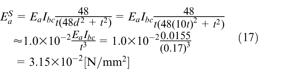
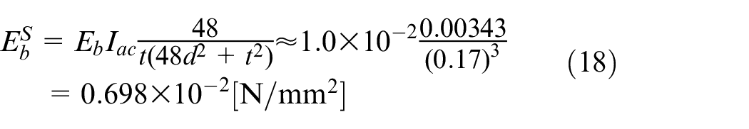
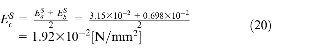
The superscript
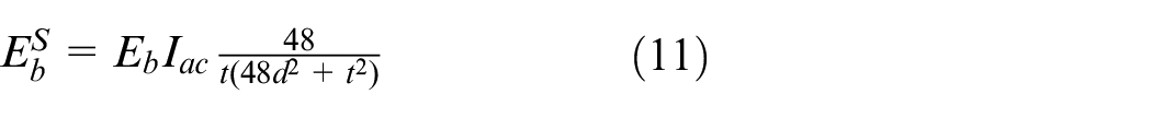
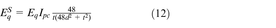
The parameter
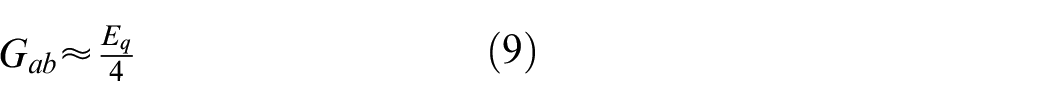
Using equation (A.10), the shear modulus
It is difficult to measure the shear modulus on the a-c or b-c plane, as shown in Figure 11. The c-axis represents the thickness direction of the fabric. In contrast, the out-plane shear stresses

The fabric analysis model exhibits a three-layer structure, as shown in Figure 20. The layer thickness of the membrane element at the center is 0.17 mm (=
The left-hand side term of the above equation represents the total mass. The right-hand side terms of the above equation represent the mass of the shell element, mass of the membrane element, and mass of the shell element, respectively. The parameters
Identification of fabric-bending stiffness
The parameter
Fabric-bending test (fabric hangs down from the block): (a) perspective view, (b) side view, and (c) side view (Horizontal distance Δx: Vertical distance Δy = 1:5.).
Parameters for identifying both the analysis and experimental results (t = 0.17 mm).
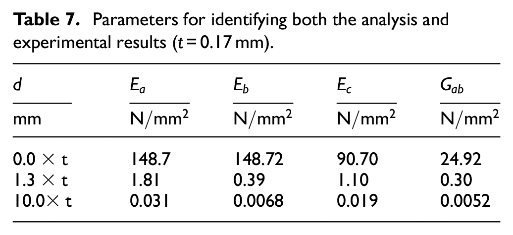
In Table 7, for example, in the case of

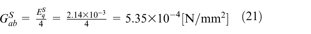
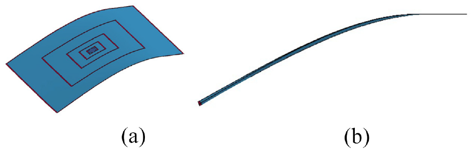
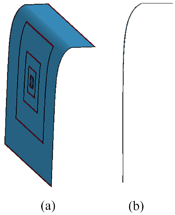
The results of the analysis conducted in the three cases using the data presented in Table 7 are shown in Figures 22 to 24. The fabric edges are fixed and subjected to gravity. The analysis results presented in Figure 22 show the condition d = 0.00
Bending state of fabric at
Bending state of the fabric at
Bending state of the fabric at
Contact analysis of LS-DYNA
A contact analysis models the phenomenon of contact and collision between multiple objects. In FEM, if the contact between objects is not defined, the objects penetrate each other without contacting each other. There are several important parameters in this contact analysis. If these parameters are not set properly, various analysis errors can occur; thus, appropriate analysis results cannot be obtained. In this section, we discuss the contact analysis of tying. The contact between the needle and fabric, that between the fabric and cap, and the self-contact of the fabric are set to analyze the tying behavior. The contact algorithm for the LS-DYNA keyword, *CONTACT_AUTOMATIC_SURFACE_TO_SURFACE 23 is applied in the tying analysis.
Master and slave
Considering the balance of forces, this mathematical equation is modeled based on FEM. The contact analysis is based on the concept of master and slave surfaces.49,50 Regarding the contact between the two objects, the distance between the surfaces of the two objects becomes zero. The nodal points on the surface of one object are projected onto the shell elements of the surface of another object. Using the normal vector created by the plane of an element on one object, the nodes on the other object are projected onto the nodes of the other element. This enables the calculation of the distance between the node and surface. The slave surface is the surface from which the nodes on the object’s surface are extracted, and the master surface is the surface from which the elements on the surface of another object are extracted. If the shape is not deformed, the normal vector created by the element plane can be evaluated with high accuracy. In this analysis, the shell elements of the fabric model cause large deformations. By inserting the shell element into the solid element that models the cap, the shell element deforms into a complicated shape. Complex shapes cannot evaluate normals with high accuracy. Therefore, the nodes on the shell element that models the fabric are set as the slave nodes, and the solid element that models the cap is set as the master nodes. The segment-based contact algorithm is applied in LS-DYNA (SOFT = 2 option 23 ).
Contact thickness
The diagram of contact thickness is shown in Figure 25. In the contact analysis, the shell element has a parameter called contact thickness. As the shell element is an element that does not have thickness, the thickness must be set. If another object (cap or needle) invades the range of the contact area (optional contact thickness for slave surface, SST 23 in Figure 25) on the shell element, the solver recognizes that an object has made contact. In this study, an explicit method is applied as the solver. In the FEM analysis, there is a concept of the time step in the time direction. If the time step decreases infinitely, the solver recognizes that the objects are in contact with each other. In contrast, the analysis time increases infinitely. To reduce the analysis time, it is necessary to take a large time step. Figure 26 shows the analysis result obtained when the contact thickness parameter SST of LS-DYNA is set to 0.04. The fabric penetrates the cap, and the moving speed of the needle is set to 30 mm/s. When the time step is set to 0.01 s, the needle moves 0.3 mm per time step. During the time interval (0.01 s) between one time step and the next, the needle passes through the contact area of the fabric (SST area, as shown in Figure 25). The contact cannot be detected. Therefore, the original thickness of the fabric, SST = 0.085, is empirically applied between the cap and the fabric. An enlarged view of the contact area between the needle and fabric is shown in Figure 27. If the needle moves at a high speed, it penetrates the fabric without detecting the contact area. The stress loaded on the fabric is reduced and cannot be calculated accurately. To analyze the high acceleration of the needle, the contact parameter between the cloth and the needle is empirically set to SST = 0.085 × 6 = 0.51. As the speed of the needle increases, the scale factor on default slave penalty stiffness (SFS) 23 between the needle and the fabric should be increased because the needle may penetrate the fabric.
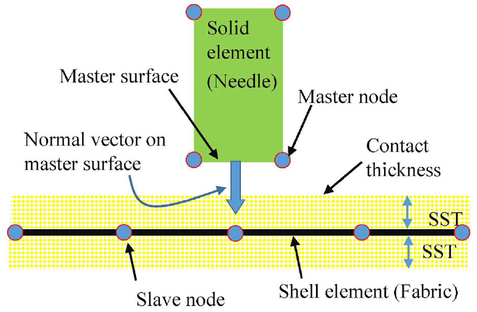
Diagram of contact thickness between the solid and shell elements.
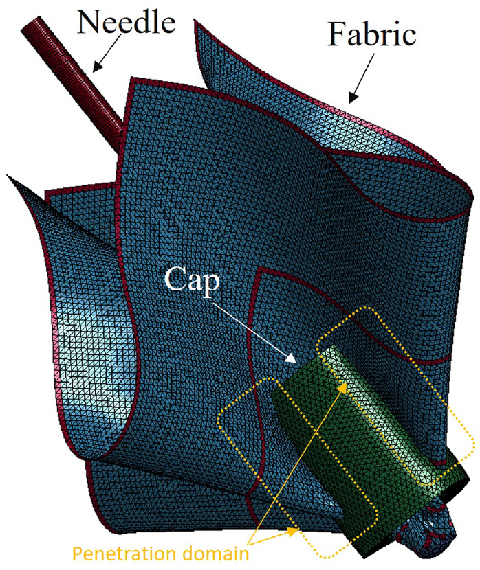
Penetration between cap and fabric (SST = 0.04).
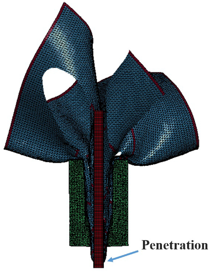
Penetration between needle and fabric (SST = 0.085).
Coefficient of friction
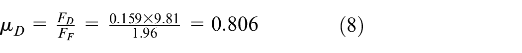
The formula for the coefficient of friction is presented in equation (22). The parameters FS and FD represent the coefficients of static friction and dynamic friction, respectively.23,51 The data in Table 4 are applicable to both FD and FS. The parameter

Viscous friction coefficient
In the tying analysis, it is necessary to set the viscous friction coefficient VC.
23
VC represents a parameter that limits the maximum value of the friction force

Here, A represents the contact area. The fabric is pulled into the cap by moving the needle. If the VC value is larger than necessary, the fabric easily sticks to the cap. Due to the strong adhesion between the fabric and cap, part of the mesh on the cap surface collapses by sliding the fabric on the cap surface. In contrast, a certain VC value is required to fix the fabric in the cap. According to the literature,23,52 the parameter VC is described as follows.
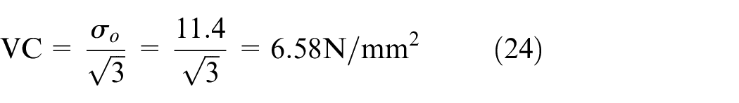
Here, the parameter
Tying analysis
Analysis model and initial conditions
Figure 28 shows the tying analysis model, which comprises the needle, fabric, and cap. Under the constraint condition, the upper surface of the cap is fixed. As an initial condition, the gap between the needle and fabric is set to 0.325 mm, and that between the fabric and cap is set to 0.18 mm. The needle moves downward, and the needle tip sticks out of the cap. Then, it returns to its initial position.
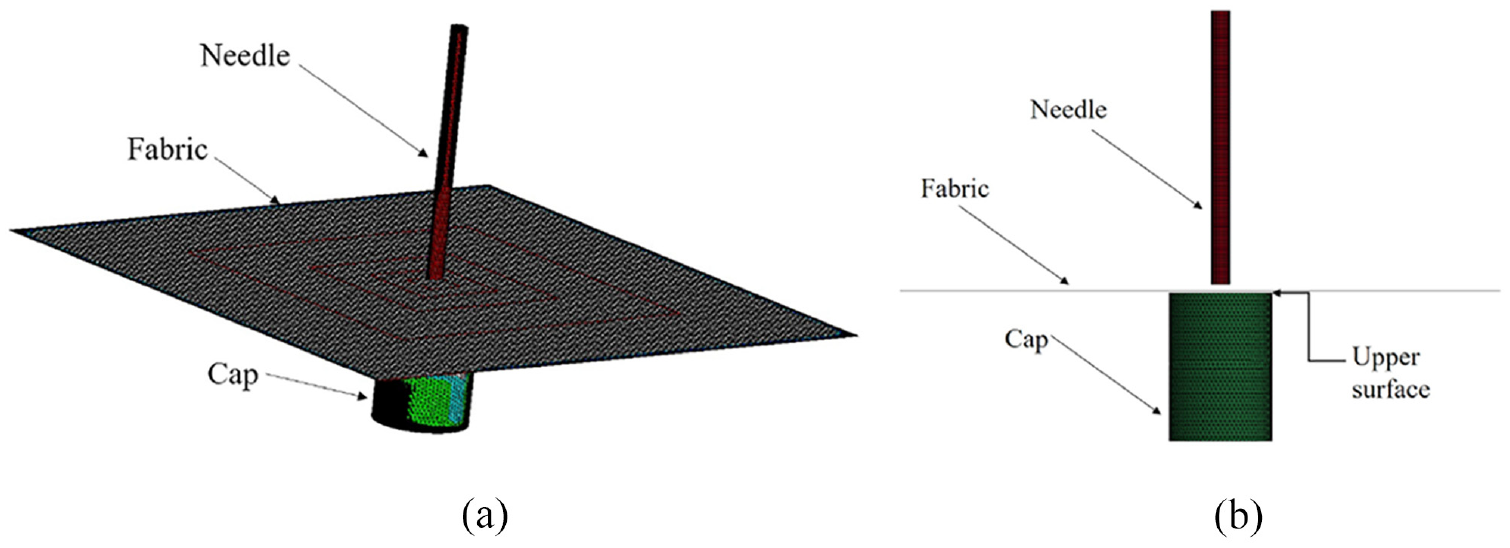
Tying analysis model (initial condition (time 0.00 s)): (a) perspective view and (b) side view.
Tying analysis results
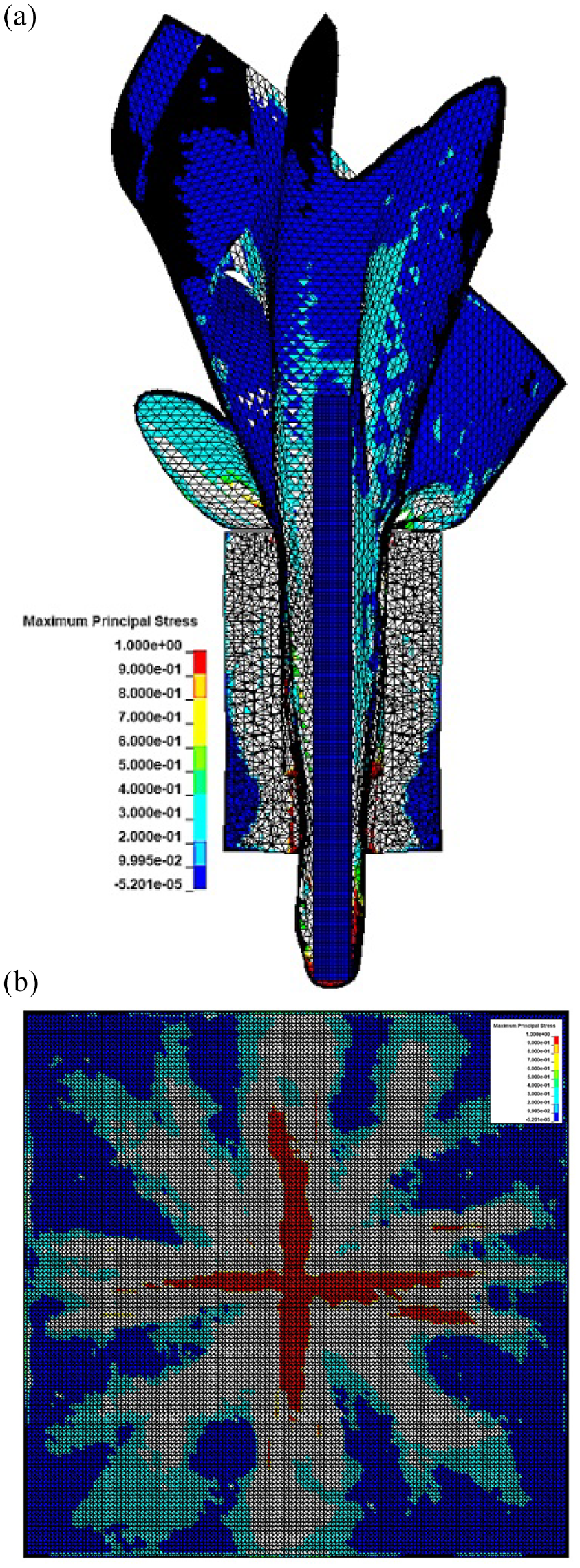
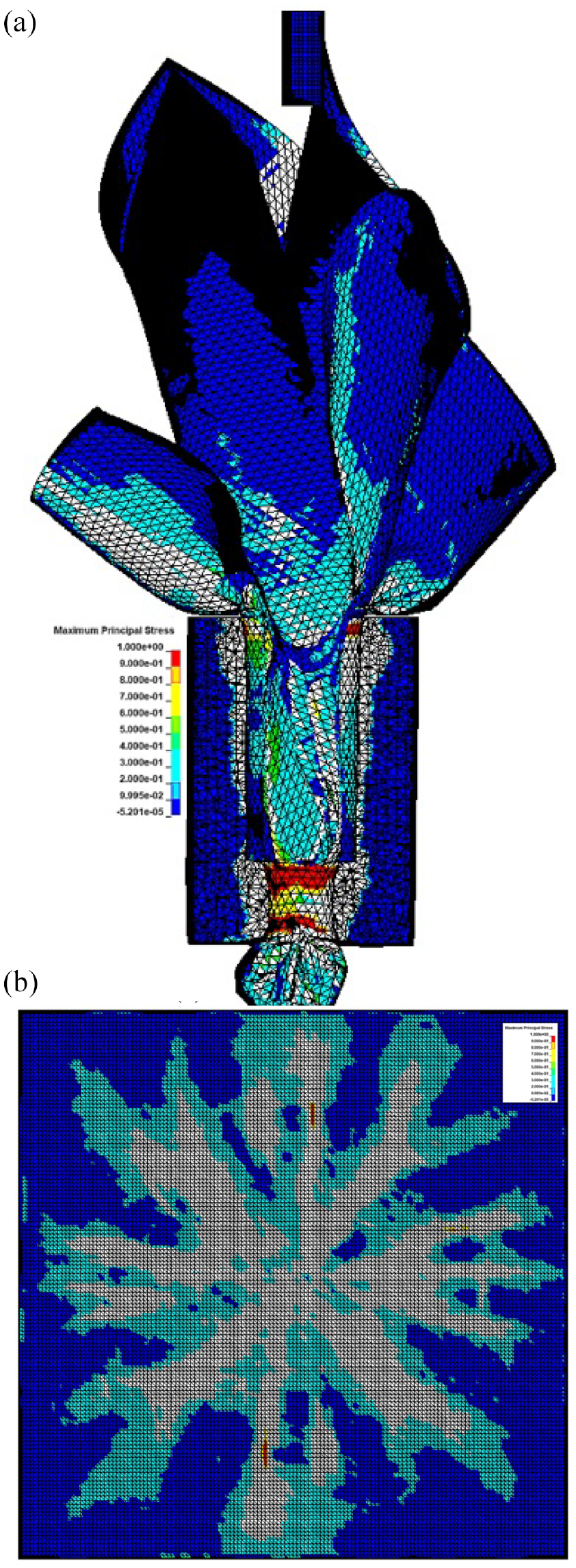
Figures 29 to 33 show how the fabric is pushed into the cap. The stress distribution on the fabric is shown in the time series. The unit of the color bar level is N/mm 2, and the acceleration of the needle is set to 33.3 m/s 2.
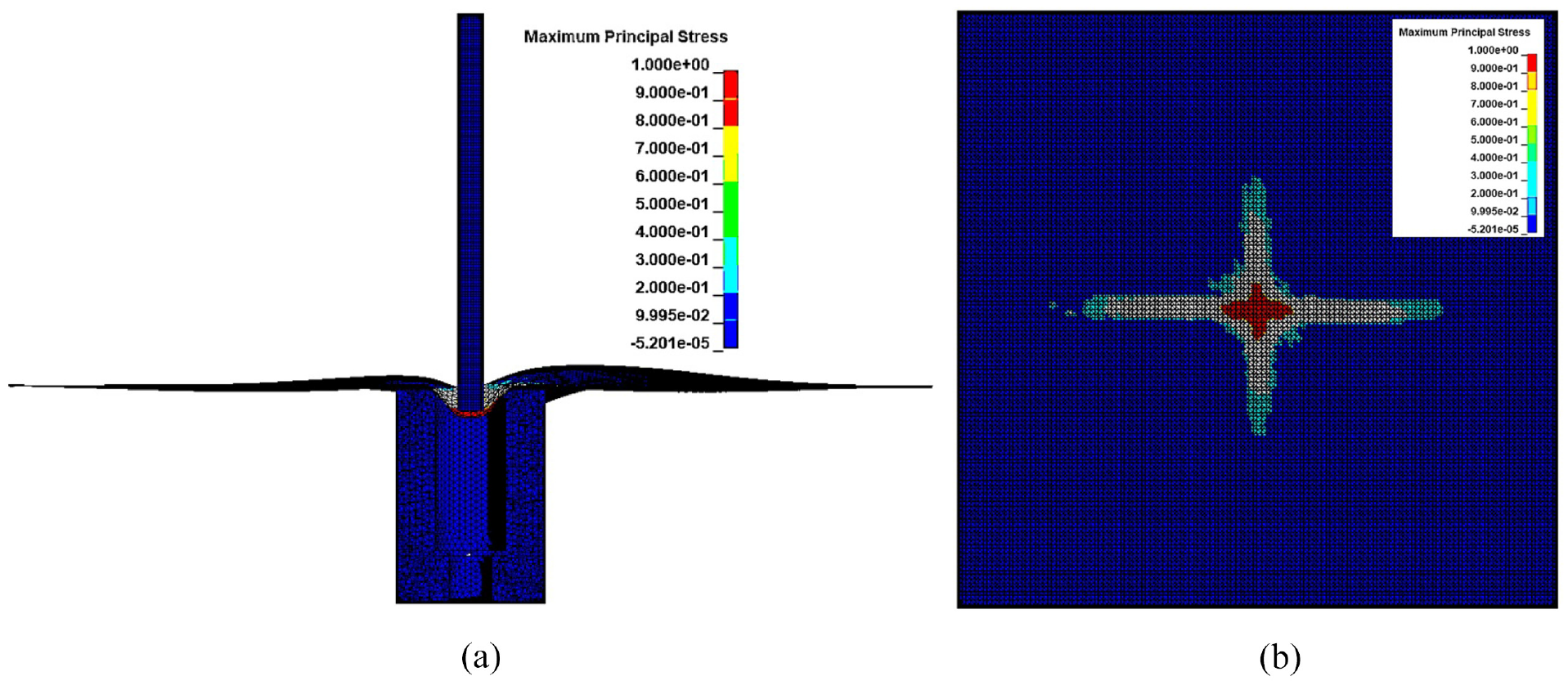
Maximum principal stress distribution of time 0.276 s after the initial condition: (a) cross section view and (b) front view of fabric.
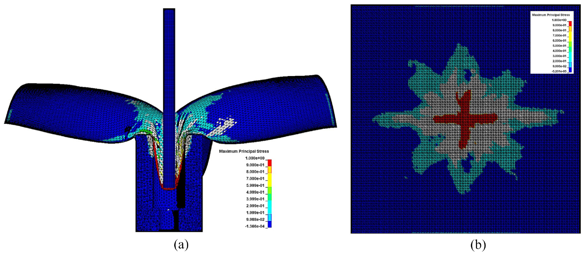
Maximum principal stress distribution at time 0.54 s after the initial condition: (a) cross section view and (b) front view of fabric.
Maximum principal stress distribution at time 0.72 s after the initial condition: (a) cross section view and (b) front view of fabric.
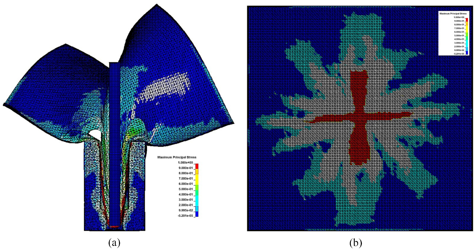
Maximum principal stress distribution at time 1.2 s after the initial condition: (a) cross section view and (b) front view of fabric.
Maximum principal stress distribution at time 2.4 s after the initial condition: (a) cross section view and (b) front view of fabric.
Figure 29 shows the stress distribution when the needle comes in contact with the fabric. The stress is concentrated near the contact area between the needle and fabric and occurs near the end of the cap that supports the fabric. The maximum principal stress induced on the fabric is 6.4 N/mm 2.
Figure 30 shows the transient state, in which the fabric is pushed into the needle cap and the flat fabric causes a complex deformation. The contact area between the fabric and cap expands, and the volume of the cavity inside the cap gradually increases as the fabric is pushed into the cap. By using a needle to press the fabric against the inside of the cap, the stress generated on both the fabric and cap surfaces is increased. The maximum principal stress induced on the fabric is 18.4 N/mm 2.
As shown in Figure 31, when the needle reaches the small diameter tube in the cap, the fabric is tightened. At this time, the fabric outside the cap enters the cap and deforms from the horizontal to vertical direction to form the tying. The maximum principal stress induced on the fabric is 21.9 N/mm 2.
As shown in Figure 32, the needle protrudes from the cap. The stress generated on the fabric and cap shows a high value as a whole. The stress generated on the fabric in contact with the needle tip reaches its maximum value, which increases the possibility of fabric breakage and maximizes the contact area between the fabric and cap. The maximum principal stress induced on the fabric is 23.8 N/mm 2. This value indicates stress near the limit at which the fabric breaks.
As shown in Figure 33, the needle is removed from the cap. The fabric is fixed by the frictional force of the cap. The stress induced on the fabric decreases when the needle is removed. The fabric stretched by the needle is rounded on the outside of the cap. The roundness forms a shape similar to that of the actual tying, as shown in Figure 5. The maximum principal stress induced on the fabric is 3.2 N/mm 2.
The time history of the maximum principal stress is shown in Figure 34. As the fabric is pushed into the cap, the contact surface between the cloth and the cap increases. As the frictional force increases under this effect, the stress induced on the fabric increases in large time increments while repeatedly increasing and decreasing in small time increments. Then, when we start pulling the needle from the cap, the stress induced on the fabric decreases rapidly. For the maximum principal stress in the cap, the stress is increased to follow the variation in the stress induced on the fabric. Next, as the needle is withdrawn from the cap, the stress induced on the cap also starts to decrease.
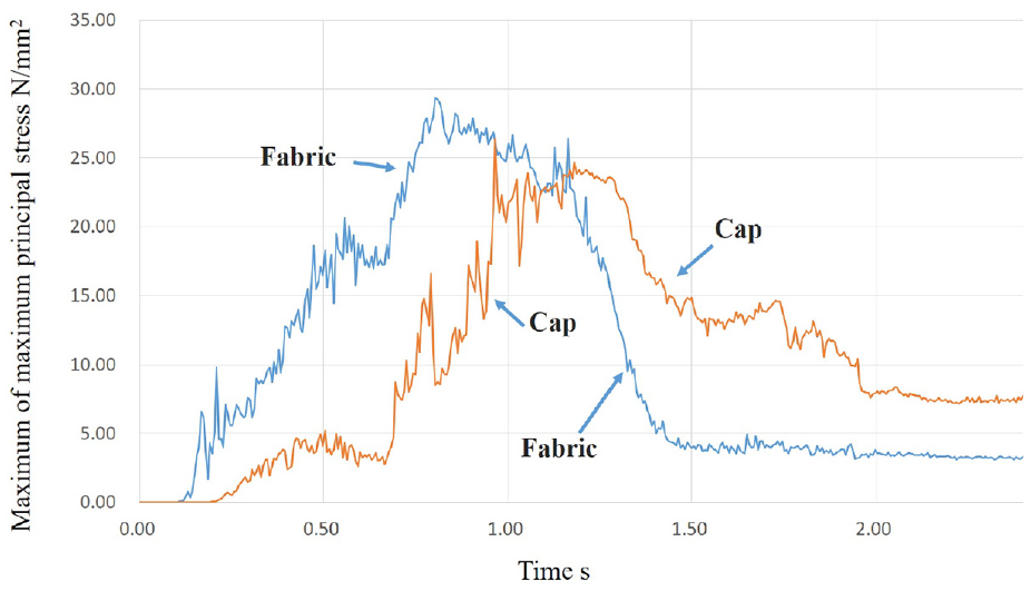
Time history of maximum of maximum principal stress with respect to a needle acceleration of 33.3 m/s 2.
The needle speed is an important issue when considering the work efficiency. As the needle speed increases, the stress induced on the fabric increases. Therefore, we study the optimum value of needle acceleration within the range in which the fabric does not break. The maximum principal stress with respect to the needle’s acceleration is shown in Figure 35. The horizontal and vertical axes represent the acceleration of the needle and the maximum principal stress induced on the fabric, respectively. The two horizontal lines in the graph represent the normal stress induced when the fabric breaks. As shown in Table 5, the breaking stress is 81.5 N/mm 2 in a-axis (Figure 11) and 40.2 N/mm 2 in b-axis. When the needle’s acceleration is approximately 700 mm/s 2, the stress loaded on the fabric reaches the breaking stress with respect to the b-axis (Figure 11). Therefore, a needle acceleration of approximately 600 mm/s 2 becomes optimal. The working time with respect to the needle’s acceleration is shown in Figure 36. As the acceleration increases, the work efficiency also increases. At the needle acceleration of approximately 600 mm/s 2, the working time is 0.5 s. Compared to the working time of 2.4 s at a needle acceleration of 33.3 mm/s 2, the working time is reduced to approximately one-fifth.
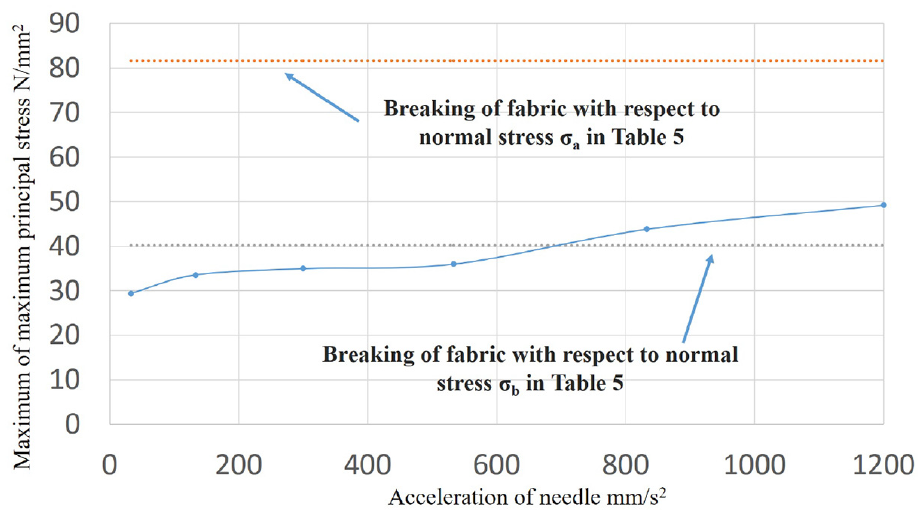
Maximum of maximum principal stress with respect to needle acceleration.
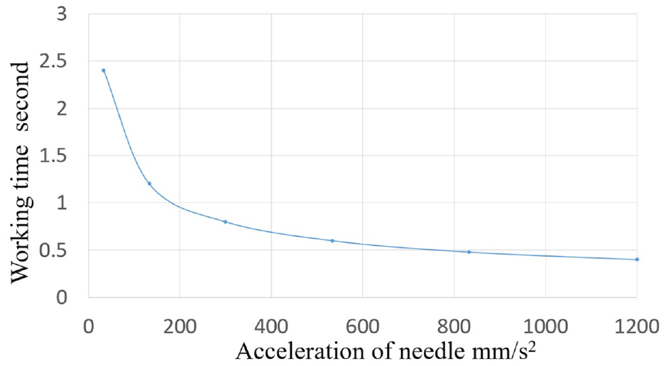
End time of work with respect to needle acceleration.
Model applicability through experiment
In this section, to verify the applicability of the model, the variation of the tying (shibori) due to the acceleration effect of the needle is visualized using a microscope. The Arimatsu Narumi shibori robot used to make the tying is shown in Figure 37.
Tying (Shibori) by Arimatsu narumi shibori robot.
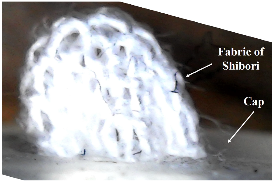
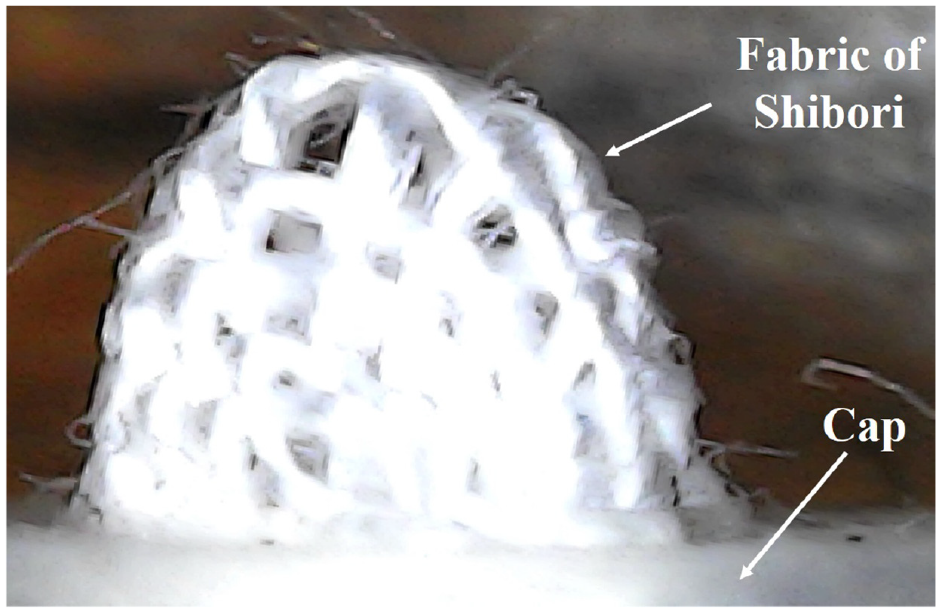
Figures 38 to 41 show the shibori parts at the needle accelerations. As shown in Table 5, the breaking stresses of the weft and warp threads are 40.21 and 81.55 N/mm 2, respectively. Observing the condition at the tip of the tied part, as shown in Figure 38, the fabric does not present any particular challenge when the needle acceleration is 33.3 mm/s 2. However, as the needle acceleration increases, misalignment or partial breakage gradually begins occurring in the fabric. To improve the quality of the Arimatsu Narumi shibori, it is necessary to suppress the misalignment that occurs between the weft and warp threads. As it is desirable to maintain an even position of the threads, the appropriate value is approximately 300 mm/s 2 or less, which is relatively free from thread misalignment.
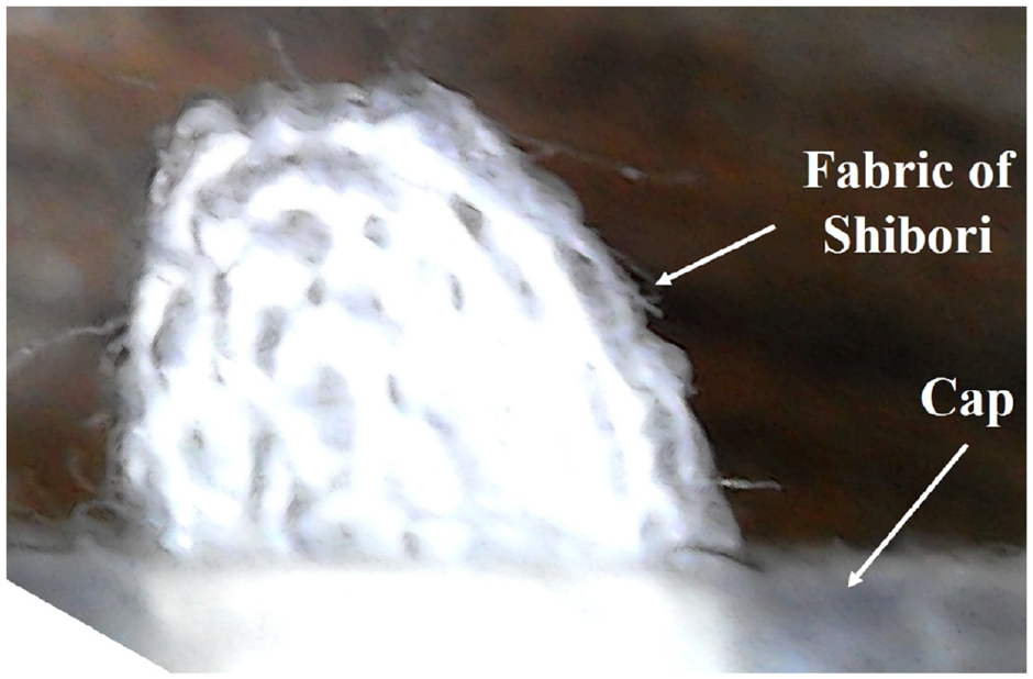
Tying (Shibori) by microscope at needle acceleration 33.3 mm/s 2.
Tying (Shibori) by microscope at needle acceleration 133.3 mm/s 2.
Tying (Shibori) by microscope at needle acceleration 300.0 mm/s 2.
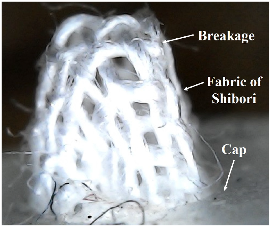
Tying (Shibori) by microscope at needle acceleration 533.3 mm/s 2.
Conclusion
To automate Arimatsu Shibori’s tying work and reproduce the dye pattern with high accuracy, we developed a robot that can reproduce Arimatsu Shibori’s tying work of Arimatsu Shibori. The tying work was reproduced by sandwiching the fabric between the cap and needle. The dye pattern was created by immersing the tying part in a dye. To predict the tying behavior, which affects the dye pattern of Arimatsu Narumi Shibori, we used, for the first time, a tying modeling method. The following conclusions were drawn.
To improve the workability and expandability for the practical use of Arimatsu Narumi Shibori, we developed an Arimatsu Narumi Shibori robot. This robot comprises mechanical elements, such as linear and rotary actuators and electronic circuits. The Arduino Mega was implemented as a microcomputer.
To develop the tying analysis modeling method, material properties were verified through tensile and friction tests conducted among the fabric, cap, and needle. To simulate the actual behavior of the fabric, we implemented a three-layered shell model. Based on the stiffness evaluation performed by tensile and bending tests, we proposed an identification method to convert the stiffness of the fabric into that of its three-layer shell.
The optimum acceleration of the needle was set to 600 mm/s 2 to shorten the working time under the condition that the fabric used in Arimatsu Narumi Shibori does not break.
By using the tying modeling method described above, we could predict the forms of fabric-tying based on the cap shape and visualize the stress distribution in the fabric. To prevent the fabric from tearing, the appropriate descent rate of the needle could be studied. This also enabled to analyze the appropriate shape of the cap to approach the tying formed by the artisan. In the future, using this analytical model, we will clarify the correlation between the stress distribution of the fabric and the osmotic pressure of the dye. We will discuss the dye fabric pattern obtained through the combination of the resist dye area and the dye area.
Footnotes
Appendix A
Acknowledgements
Declaration of conflicting interests
The author(s) declared no potential conflicts of interest with respect to the research, authorship, and/or publication of this article.
Funding
The author(s) received no financial support for the research, authorship, and/or publication of this article.