Sage Journals: Discover world-class research

Abstract

A new structure is proposed for a DN25-type ultrasonic gas flow meter with a V-shape double sound channel arrangement. The flow field characteristics are analyzed including velocity curves for the four channel lines, velocity profiles for different cross-sections of the flow meter, and streamlines of the transducer channel sections. The metering characteristics of the flowmeter are measured using a Venturi nozzle device. When the pipeline flow rate is less than 2.26 m/s, the pipe installation does not have a significant effect on the velocity profile and the velocity in the channel lines. However, the error in the low-flow region is large, and the flow distortion directly affects the measurement accuracy. When an ultrasonic gas flow meter with an accuracy class of 1.5 is used with pipes containing a single or double bend upstream, the linear error doubles, low-flow error becomes a negative deviation, and reference error in the low-flow region becomes approximately 700%–949%. The installation structure of the first pair of transducers also affects the signal propagation of the transducers behind it. Therefore, it is critical to process the ultrasonic signal according to the flow field distribution and adopt different weighted algorithms to obtain accurate pipeline flow rates to improve the measurement accuracy of the ultrasonic flow meter.

Keywords

Measurement characteristics numerical simulation ultrasonic gas flow meter small-bore

Introduction

The natural gas market is developing rapidly; therefore, there is an increasing demand for accurate and reliable natural gas measurements. Moreover, the automation of trade measurement and station control systems requires flow meters with high precision and wide measurement ranges that effectively reduce the transmission difference. Recently, ultrasonic gas flow meters have been developed. These new meters have a low minimum flow rate, wide range, high precision, no moving parts, self-diagnostic functions, and bidirectional measurement capability. They have been widely compared with turbine and root gas flow meters, which are in widespread use. However, ultrasonic gas flow meters are not broadly applied in gas transmission pipelines because of limitations in field adaptability, ultrasonic transducer techniques, and signal processing technology, as well as the fact that ultrasonic propagation characteristics affect their accuracy.

Currently, most ultrasonic gas flow meters use the transit-time method, where the time interval of acoustic propagation is measured and used to calculate the fluid velocity in the sound channel, which is then converted to the pipe velocity. Therefore, the flow field is a crucial factor, and the medium flow state directly affects the propagation path of sound waves. Hence, ultrasonic gas flow meters require uniform and stable pipe flow, which can be achieved if the pipe upstream from the meter is long and sufficiently straight. Many standard specifications state that there should be at least 10D–20D of straight pipe upstream without a rectifier,¹ and 5D of straight pipe with a rectifier at the inlet. In reality, the installation space is often insufficient for such a straight pipe, and flow meters are installed directly behind obstructions that produce turbulence, such as single bends, double bends, or tee joints. Turbulence introduces a radial velocity component perpendicular to the pipe axis, in addition to the flow velocity along the pipe, such as the secondary flow observed at the rear of a bend. Consequently, the symmetry of the ideal flow field is destroyed, thereby changing the propagation direction and velocity of sound waves and affecting the acoustic wave alignment and counter current propagation time collected by the flow meter.² Tang³ and Chen⁴ used the flow field characteristics and ultrasonic flow meter analysis to provide a reference for the position of flow meter installation. Moreover, the signal processing technology and methods required to achieve relatively accurate measurements through effective processing and modification of ultrasonic signals under complex flow field have been researched extensively.^5,6 For example, a new signal processing method was proposed to determine the transit time difference, particularly at lower signal-to-noise ratios, and to improve the accuracy of transit time difference estimations using clamp-on time-of-flight ultrasonic flow meters for wet stream flows.⁷ A method of modeling the received ultrasonic signal using variable frequency analysis was also proposed and validated for an ultrasonic gas flow meter. In this method, the traditional exponential model was modified to include a time-variant frequency parameter, whose value can be estimated based on the sampled signal using the Teager energy operator.⁸ The propagation characteristics of ultrasonic waves^9,10 and the coupling of flow and sound fields have also been investigated.^11,12 A large-diameter multi-channel ultrasonic gas flow meter was designed to improve the measurement accuracy by expanding the sound channels or changing their arrangement to extend the ultrasonic propagation path.¹³ Recently, a new hybrid scheme combining computational fluid dynamics (CFD), wave acoustics, and ray acoustics was proposed.¹⁴ Furthermore, a flow field with a vortex near the transducer and its effect on sound propagation, reception, and flowmeter performance were analyzed in depth.

Modules for an multipath ultrasonic gas flowmeter, including the acoustic path arrangement, ultrasound emission and reception module, transit-time measurement module, and software, were designed by Chen et al.¹⁵ The effects of ultrasonic noise generated by pressure control valves on ultrasonic gas flowmeters were investigated by Kang et al.¹⁶ To consider the effects of a non-uniform flow profile, a semi-3D simulation technique was used, and the flow profile correction factor for a commercial ultrasonic meter was calculated with reasonable accuracy for different inlet flow velocities.¹⁷ The inherent error of an ultrasonic flowmeter with non-ideal hydrogen gas flow was researched by Chen and Wu.¹⁸ They used CFD to simulate hydrogen flows downstream from a single right bend and an orifice plate at different Reynolds numbers. The results showed that the errors increased when the flowmeter was closer to the disturbance sources. However, increasing the number of acoustic paths can effectively reduce the errors caused by a non-ideal flow.

It is more difficult for small-diameter ultrasonic flow meters to achieve high precision measurements. Therefore, this study presents a design for a two-channel ultrasonic gas flow meter with DN25 diameter, and the flow field and measurement characteristics under different pipe installation conditions are investigated.

Theory and design

Measurement principle of ultrasonic flow meter

Transit-time method ultrasonic flow meters are velocity flow meters that obtain the gas flow rate by measuring the time difference in the propagation of high-frequency pulses.¹⁹ A pair of ultrasonic transducers is installed on either side of the tube wall at angle θ, and they transmit/receive ultrasonic pulses to/from each other simultaneously. The upstream and downstream wave propagation velocities are different, and this difference can be used to calculate the flow velocities. A schematic diagram of the arrangement is shown in Figure 1.

Figure 1.

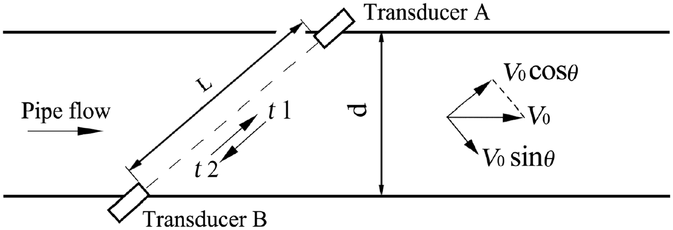
Schematic diagram showing the arrangement used to calculate the flow velocities, t₁ and t₂ are the downstream and upstream propagation times, respectively.

The downstream and upstream propagation times of the ultrasonic wave, t₁ and t₂ respectively, are given by

t_{1} = \frac{L}{c + v_{0} \cos θ},

(1)

and

t_{2} = \frac{L}{c - v_{0} \cos θ},

(2)

where c is the sound velocity, L is the length of the ultrasonic channel, θ is the angle between the sound channel and the pipe axis, and v₀ is the mean velocity of the pipe flow given by

v_{0} = \frac{L}{2 \cos θ} (\frac{1}{t_{1}} - \frac{1}{t_{2}}) .

(3)

During gas transmission, the velocity of the gas in the pipeline is not uniform, and small changes in the external environment can cause substantial fluctuations and distortions. This makes it difficult to measure the real mean velocity of the pipe flow using single-channel ultrasonic flow meters, particularly those used in large-diameter pipelines where the measurement error is significantly increased. Multi-channel measurements can be used to refine the mean pipe flow velocity, and improve the accuracy of the results. A commonly used four-channel ultrasonic flow meter is considered as an example, and the sound channel layout is shown in Figure 2.

Figure 2.

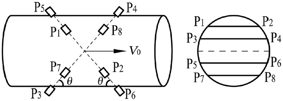
Sound channel layout for a four-channel ultrasonic flow meter, P₁–P₈ are the transducers.

The multi-channel ultrasonic flow meter also uses the acoustic time difference method. The flow velocity for each channel is

v_{i} = \frac{L_{i}}{2 \cos θ_{i}} (\frac{1}{t_{1 i}} - \frac{1}{{t_{2}}_{i}}),

(4)

where i is the sequence of the sound channel (i = 1, 2, 3, 4); L_i and θ_i are the length (m) and inclination angle of channel i, respectively; and t_1i and t_2i are the downstream and upstream propagation times in channel i, respectively. The flow velocity of the gas through the pipe section can be obtained from the weighted integral of the flow velocity in each channel²⁰:

v_{0} = \sum_{i = 1}^{4} w_{i} v_{i},

(5)

where w_i is the weighted factor for channel i. The instantaneous volume flow, Q, is given by

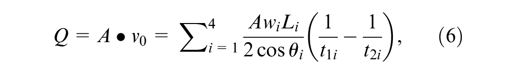
Q = A • v_{0} = \sum_{i = 1}^{4} \frac{A w_{i} L_{i}}{2 \cos θ_{i}} (\frac{1}{t_{1 i}} - \frac{1}{t_{2 i}}),

(6)

where A is the cross-sectional are of the pipe.

Two-channel structure design

The structure of the two-channel ultrasonic DN25 gas flow meter is shown in Figure 3. It consists of primary and secondary instruments. The primary instrument is mounted on the pipe with the fluid flowing through it. The secondary instruments, also called intelligent flow integrators, are installed on the primary instrument or remotely. They process and communicate the signals collected by sensors on the primary instrument, display information on an LCD, and communicate with the control center and user by a variety of means such as RS485 and the internet of things. The structure of the primary instrument is the main focus of this study. The flow range was designed to be 0.5–40 m³/h.

Figure 3.

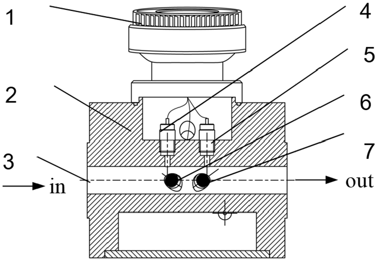
Cross-section of the ultrasonic gas flow meter: (1) intelligent flow integrator, (2) mechanical shell, (3) flow channel, a through-hole with a diameter of 25 mm, (4) pressure sensor, (5) temperature sensor, and (6, 7) two pairs of transducers. (4–7) Are mounted on the mechanical shell. When the fluid flows in, the sensors detect and transfer signals to the intelligent flow integrator.

Small-diameter ultrasonic flow meters, such as the DN25 type, have short sound channels, and low temporal resolution. To extend the sound channel line, V-shaped sound channels and two-channel structures were adopted, as shown in Figure 4. The sensors were mounted without protrusion.

Figure 4.

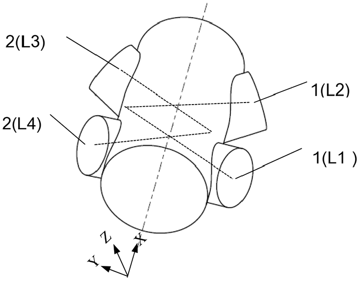
Schematic diagram of the sound-channel layout with two V-shaped channels (1 and 2), each with two transducers (A and B) that send signals to each other alternately.

The flow meter has two sound channels (1 and 2), each of which have two transducers that send signals to each other alternately. Sound channel 1 consist of path L1 and L2, and sound channel 2 consist of path L3 and L4.The arrangement of the sensors in channel 1 and channel 2 is symmetric with respect to the vertical middle section of the pipeline. The angle of the center line of the sensors at the transmitting and receiving ends of each channel is determined in combination with the installation size. In this case, the angle between the center lines of the two sensors is 108°.

Numerical simulation

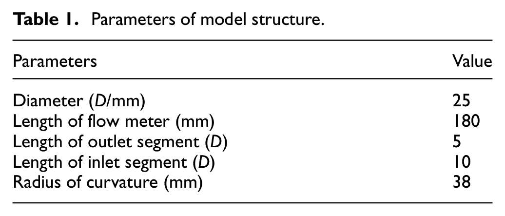
CFD was used to analyze the flow field of the ultrasonic flow meter. The physical model consists of a pipe section containing inlet, flow meter, and outlet segments. Three models were used depending on the pipeline installation: long straight pipe (Condition I), 90° bend (Condition II), and double bend (Condition III) without co-planar at the inlet segment, as shown in Figure 5. Parameters of the model structure are shown in Table 1.

Figure 5.

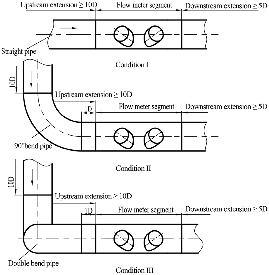
Computational models used for different pipeline installations.

Table 1.

Parameters of model structure.

Parameters	Value
Diameter (D/mm)	25
Length of flow meter (mm)	180
Length of outlet segment (D)	5
Length of inlet segment (D)	10
Radius of curvature (mm)	38

Model and numerical method

The commercial CFD software, ANSYS FLUENT v16, was employed to solve the three-dimensional incompressible Navier–Stokes equations. The pressure–velocity coupling was calculated based on the SIMPLEC algorithm. Second-order upwind discretization was used for the convection and central difference schemes in the diffusion terms. The residual criterion was set to 1e−5. The realizable k–ε turbulence model was used for the ultrasonic flow meter calculation under the influence of secondary flow.

Boundary conditions and grid

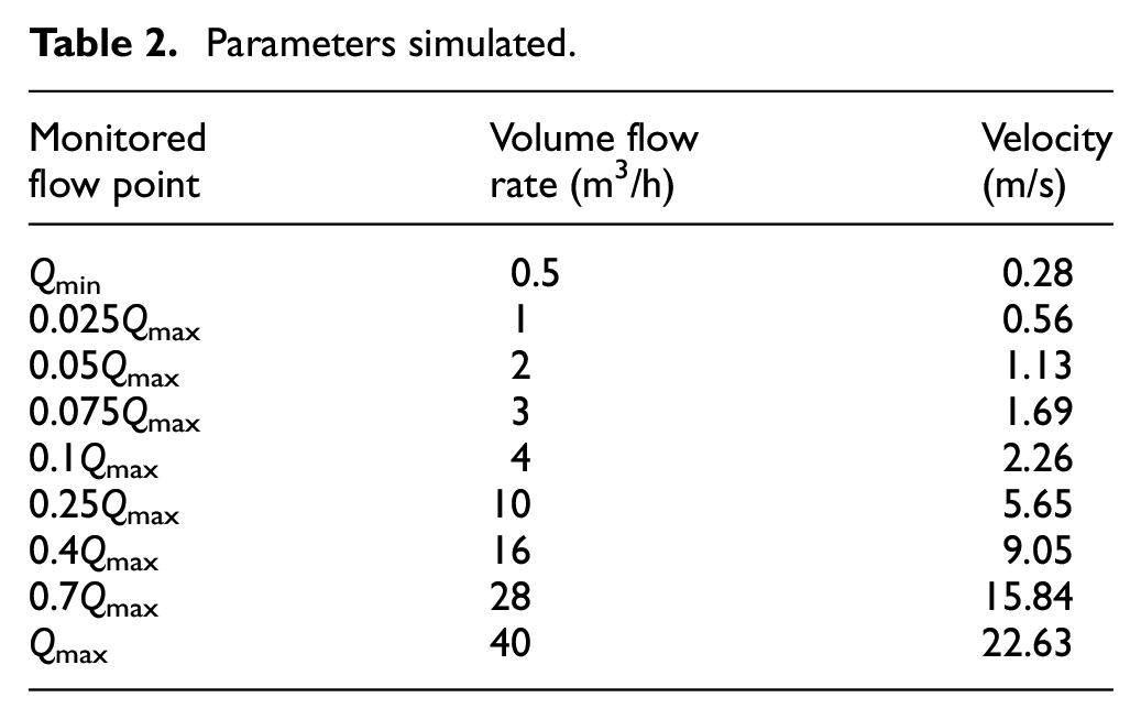
Velocity inlet boundary conditions were applied at the pipe inlet. The inlet velocity was calculated according to the volume flow rate and pipe diameter. Outflow boundary conditions were adopted at the pipe outlet. Nonslip boundary conditions were used for the near-wall function. A typical structured hexahedral mesh was generated for the entire computational domain, the grid of the ultrasonic gas flow meter region consisted of 979916 elements and 951481 nodes, as shown in Figure 6. The simulation was performed for nine flow points, as shown in Table 2.

Figure 6.

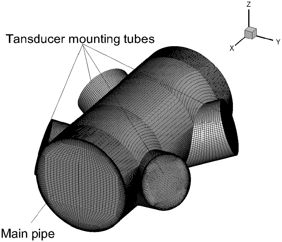
Computational domain of the ultrasonic gas flow meter.

Table 2.

Parameters simulated.

Monitoredflow point	Volume flowrate (m³/h)	Velocity(m/s)
Q _min	0.5	0.28
0.025Q_max	1	0.56
0.05Q_max	2	1.13
0.075Q_max	3	1.69
0.1Q_max	4	2.26
0.25Q_max	10	5.65
0.4Q_max	16	9.05
0.7Q_max	28	15.84
Q _max	40	22.63

Results and discussion

Velocity distribution curve under different installation conditions

The flow field distribution varies depending on the installation conditions, so the velocity distribution curves for the flow meter inlet were analyzed under different conditions, as shown in Figure 7. Under condition I, when the straight pipe upstream was sufficiently long, the flow field was fully developed, and the flow profile in the flow meter was uniform. The velocity distribution curve in the cross-section of the inlet was U-shaped. Under condition II, secondary vortex flow formed and the velocity curve became M-shaped. Under condition III, the velocity curve was more distorted, similar to a ladder, the velocity along the z-axis was greater than the average flow velocity, and the negative velocity along the z-axis was significantly lower than the average flow velocity. This occurred due to secondary vortex flow caused by the double bend.

Figure 7.

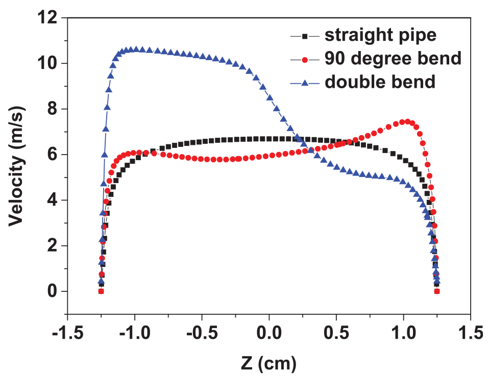
Velocity at the flow meter inlet for installations with a long straight pipe (condition I), a pipe with a 90° bend (condition II), and a pipe with a double bend (condition III).

Velocity on sound channel path

The proposed ultrasonic gas flow meter has two sound channels consist of four channel paths, and the channel velocities were computed for each of the three conditions, as shown in Figures 8 to 10. The velocity curves are N-shaped with turning points at the far right caused by the flow in the mounting hole of the sensor. Under condition I, the velocity curve for each channel was nearly the same, indicating that the velocity distribution was uniform and unrelated to the inlet velocity. Under condition II, channel paths L₁ and L₄ had the same velocity, and channel paths L₂ and L₃ had the same velocities. This occurred for the same reason channel paths L₁ and L₂ have the same x-coordinates, they are symmetric with respect to the y–z plane and the flow direction is along the positive x-axis. When the pipe inlet velocity was less than 9.05 m/s, the velocity in the different channel paths was similar and relatively stable, but when it was larger, the velocities varied significantly between the channel paths, except at the edges. The fluid flow rates in channel paths L₂ and L₃ were less than those in channel paths L₁ and L₄. This is because the fluid passed through channel paths L₁ and L₄ before channel paths L₂ and L₃, due to the mounting effect from the front pair of sensors which caused the fluid flow to the rear sensors to slow down. Peaks appeared on the left side of the velocity curves.

Figure 8.

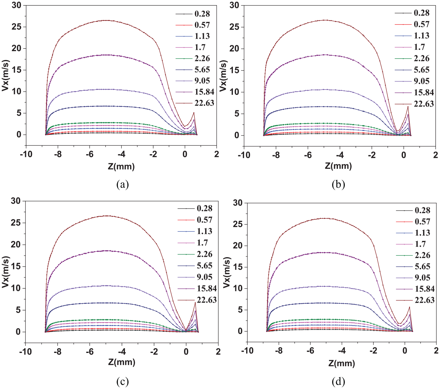
Velocity along sound channel paths with different pipe inlet velocities (condition I): (a) velocity along sound channel path L₁, (b) velocity along sound channel path L₂, (c) velocity along sound channel path L₃, and (d) velocity along sound channel path L₄.

Figure 9.

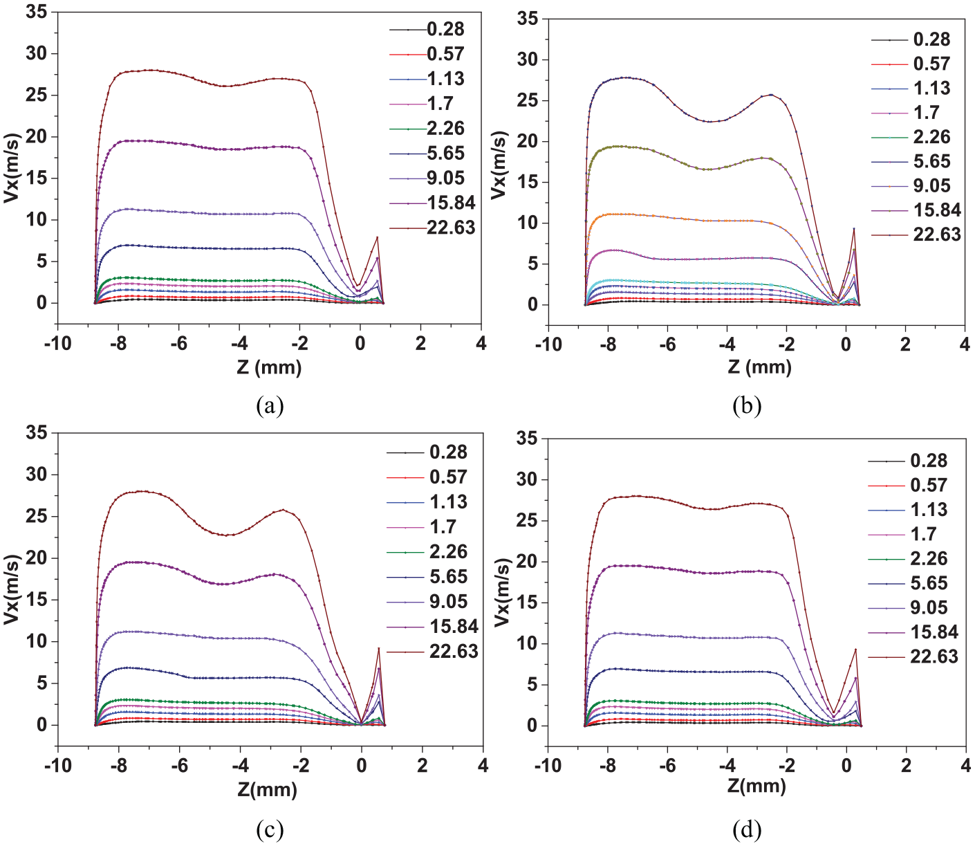
Velocity along sound channels with different pipe inlet velocities (condition II): (a) velocity along sound channel path L₁, (b) velocity along sound channel path L₂, (c) velocity along sound channel path L₃, and (d) velocity along sound channel path L₄.

Figure 10.

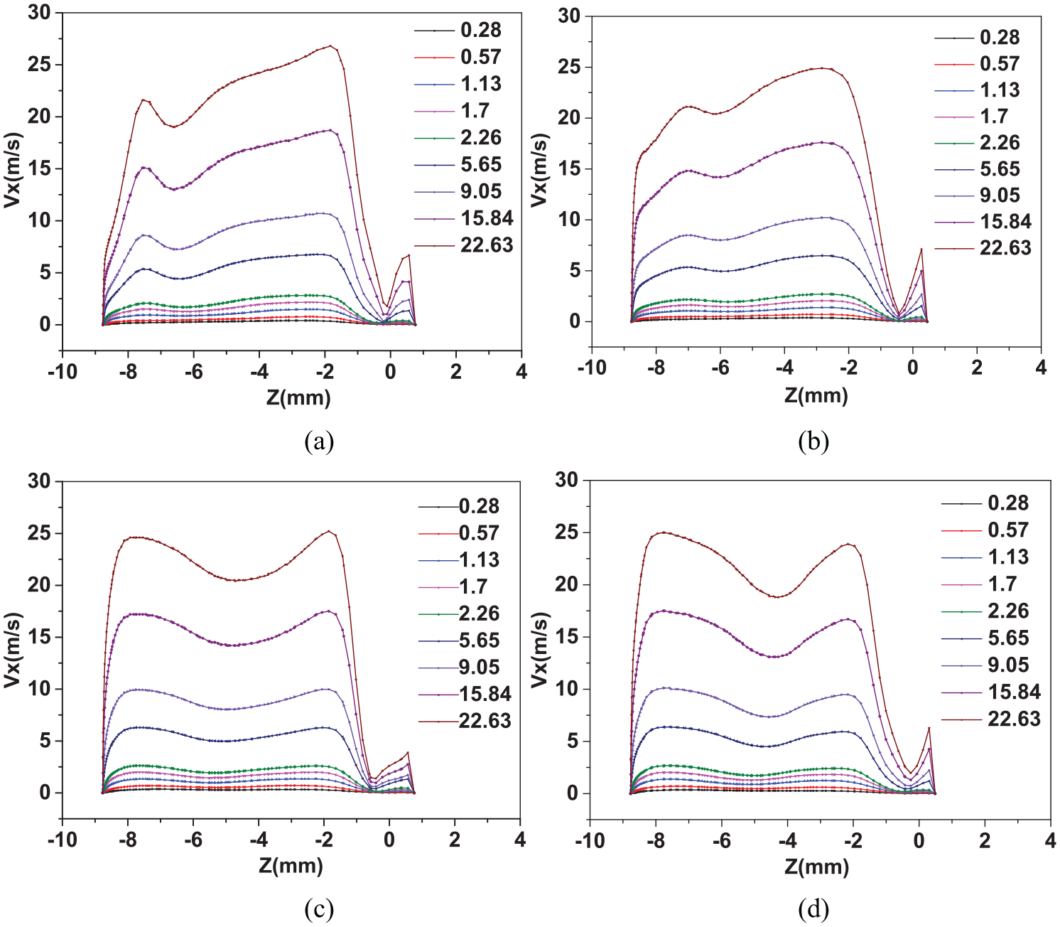
Velocity along sound channel paths with different pipe inlet velocities (condition III): (a) velocity along sound channel path L₁, (b) velocity along sound channel path L₂, (c) velocity along sound channel path L₃, and (d) velocity along sound channel path L₄.

Under condition III, the velocity in each channel path was different. The velocities in channel paths L₁ and L₂ were similar, and those in channel paths L₃ and L₄ were similar. As the pipe flow rate increased, the velocity curves changed substantially to an M-shape, and two peaks formed. Thus, using a weighted average algorithm, it should be different for each channel path.

Velocity contour in x-direction at the ultrasonic gas flow meter section

Considering an inlet velocity of 5.65 m/s as an example, the velocity distribution contours at cross-sections between the inlet and outlet of the flow meter were analyzed. As shown in Figure 11, under condition I the velocity distribution was relatively uniform across each section of the main pipe. The maximum velocity occurred at the center of the pipeline, and it was symmetric with respect to the xy-section. Under condition II, the maximum velocity changes from the negative z-direction to the positive z-direction from the inlet to the outlet of the flow meter. The velocity distribution is approximately symmetrical on both sizes of the xz-section. Under condition III, the maximum velocity is deflected from the negative y-direction to the positive y-direction. Under all three conditions, the velocity inside the sensor installation tube gradually decreased to zero, and the velocity distribution at the second pair of transducers was different from that at the first pair of transducers. It can be seen that the flow at the second pair of transducers was affected by the installation effect of the first pair of transducers.

Figure 11.

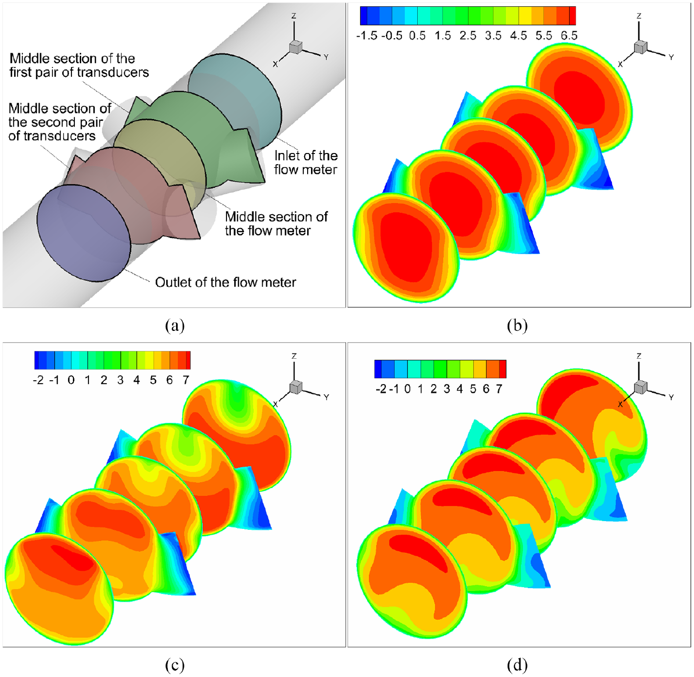
Contour of velocity in x-direction at cross-sections of the ultrasonic gas flow meter (inlet velocity 5.65 m/s): (a) position of the slices, (b) condition I, straight pipe, (c) condition II, 90° bend, and (d) condition III, double bend.

Streamlines in the x-direction cross-sections

The streamline distribution at each cross-section shown in Figure 11(a) (except the flow meter outlet), was analyzed for the three operating conditions, as shown in Figure 12(a) to (l). The installation structure of the first pair of transducers affected the streamline distribution from the inlet of the flow meter and caused multiple eddies. Thus, the streamline distribution at the second pair of transducers was different from that at the first pair of transducers. These factors affected the propagation of ultrasonic signals in the fluid.

Figure 12.

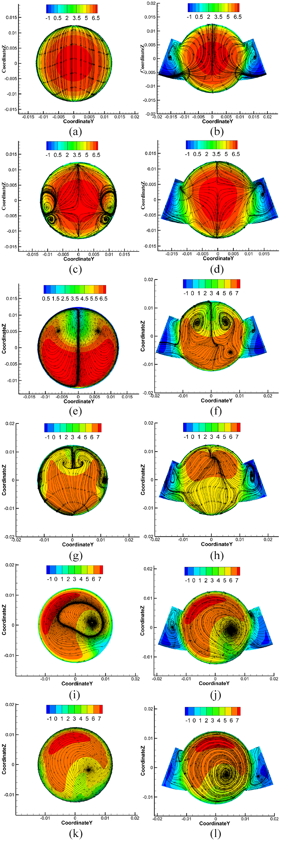
Streamlines for the inlet, first transducer, middle, and second transducer cross-sections shown in Figure 11(a) for (a–d) condition I, (e–h) condition II, and (i–l) condition III.

Streamlines in the section along the channel line

The streamlines in cross-sections along the channel under the three operating conditions are shown in Figure 13. In each case, vortex flow occurred at the sensor locations. Considering the background velocity contours and streamlines, under condition I, the velocity distribution in the mainstream was uniform without radial separation. Under condition II, when the flow passed the first pair of sensors, the velocity decreased before reaching the second pair of sensors. Under condition III, the direction of flow velocity in the main channel changed significantly and the value decreased. The velocity along the channel line decreased gradually in the direction of signal propagation. It can be seen that the pipe with a double bend (condition III) caused the greatest flow field distortion. Moreover, the velocity in each channel was different, so the method used to calculate the pipeline velocity should be different.

Figure 13.

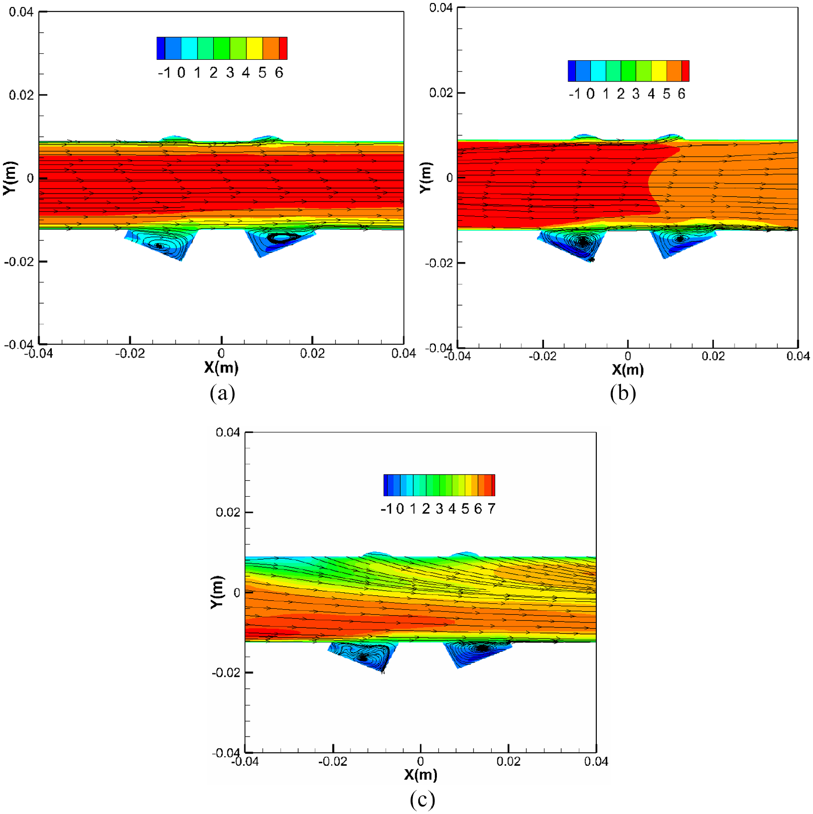
Streamlines in a cross-section along the channel line for: (a) condition I, (b) condition II, and (c) condition III.

Experimental details

The measurement characteristics test for the ultrasonic flow meter was conducted using a Venturi nozzle method gas flow standard device (shown in Figure 14). It executed quantity traceability and quantity value transfer with an uncertainty of 0.2%. After device verification, coefficient K was obtained, which is the core parameter determining the metering accuracy of the flow meter. It is defined as the number of signal pulses sent by the flowmeter, or the frequency of the pulse sent per unit volume of fluid flowing past. It can be expressed as²¹

K = N / V = f / Q_{v}

(7)

where K (1/m³), N is the number of pulses, V is the volume flow past the flow meter (m³), f is the frequency of the pulse sent (Hz), and Q_v is the volume flow rate past the flow meter (m³/s).

Figure 14.

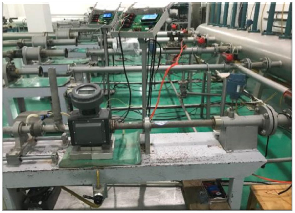
Photograph of the test device.

The flow signal measured by the flowmeter was converted into a pulse signal by signal processing, and the meter coefficient was calculated. The meter coefficient curve was drawn for a multi-point test within the flow range, and the measurement accuracy was calculated. The K coefficients for the three working conditions tested are shown in Figure 15. A key parameter for determining the metering performance is linear error δ, which is given by

δ = \pm \frac{K_{\max} - K_{min}}{K_{\max} - K_{min}} .

(8)

When the weighted average algorithm for the average pipeline velocity was kept constant in the linear region (0.1Q_max–Q_max), the K coefficient was the highest for condition I (straight pipe) and lowest for condition II (90° bend). This indicates that the number of pulses measured by the sensor is reduced when the flow state changes. The linear errors for the three conditions are shown in Table 3. The linear error in the linear region was within ±1.5%, meeting the requirement of an accuracy class of 1.5 for the measuring instrument. However, there was a significant error in the lower flow range due to the effect of the fluid on the ultrasonic propagation and the nature of the ultrasonic waves.

Figure 15.

Curves showing the K coefficient at different flow rates for conditions I–III.

Table 3.

The linear error and reference error with different upstream.

Flow range	Linear error, δ (%)			Reference error, e (%)
Flow range	Straight pipe	90° bend	Double bend	90° bend	Double bend
0.1Q_max–Q_max	0.77	1.18	1.18	53	53
Q _min–0.1Q_max	2.57	−15.60	−21.82	707	949

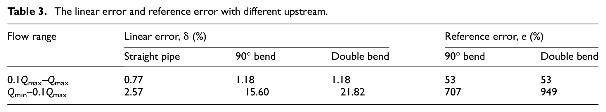
When a gas ultrasonic flow meter with an accuracy class of 1.5 was used under conditions II and III, the linear error doubled, the low flow error showed a negative deviation, and the reference error in the low flow rate region was approximately 700%–949%. The flow field distortion especially affected the propagation trajectory of the ultrasonic wave in the low flow rate region.

Conclusion

The environment in which ultrasonic gas flow meters would be used cannot satisfy the requirement for straight pipe sections, and the flow field is distorted by pipeline installations. Case studies show that when an ultrasonic gas flow meter with an accuracy class of 1.5 is used where there is a single or double bend in the upstream pipe, the linear error doubles, low flow error becomes a negative deviation, and reference error becomes approximately 700%–949%. Therefore, the K coefficient should be adjustable. When a multi-channel design is adopted, the weighted algorithm for the pipeline velocity calculation should be different, because the velocity on each sound channel is different, particularly when the flow rate is high. Applicable CFD numerical simulation technology is available, and it can predict the effect of the flow field on the measurement results, which is convenient for adopting more accurate algorithms for the subsequent signal processing process and improves measurement accuracy.

Footnotes

Appendix

Declaration of conflicting interests

The author(s) declared no potential conflicts of interest with respect to the research, authorship, and/or publication of this article.

Funding

The author(s) disclosed receipt of the following financial support for the research, authorship, and/or publication of this article: This research was supported by the National Natural Science Foundation of China (Grant No.52006198 and U1709209), the Key Research and Development Program of Zhejiang Province (2020C01027).

ORCID iDs

Desheng Chen

Haibin Cao

References

Yao

Measurement accuracy improvement method of gas ultrasonic flowmeter in complex flow field. PhD Thesis, Zhejiang University, China, 2018.

Zhang

Application of ultrasonic flow meter in chemical production unit. Equip Manag Maint 2018; 17: 118–120.

Tang

XY.

Simulation and experimental study of multichannel ultrasonic gas flow detection technology. PhD Thesis, Zhejiang University, China, 2015.

Chen

WG.

Analysis and compensation method of non-ideal flow field of gas ultrasonic flow meter. MD Thesis, Zhejiang University, China, 2015.

Piao

Yang

Kweun

, et al. Ultrasonic flow measurement using a high-efficiency longitudinal-to-shear wave mode-converting meta-slab wedge. Sens Actuator A Phys 2020; 310: 112080.

Chen

Zhang

Wang

, et al. Design of a high precision ultrasonic gas flowmeter. Sensors 2020; 20: 4804.

Murakawa

Ichimura

Sugimoto

Evaluation method of transit time difference for clamp-on ultrasonic flowmeters in two-phase flows. Exp Therm Fluid Sci 2019; 112: 109957.

Fang

Qin

, et al. Modelling of received ultrasonic signals based on variable frequency analysis. Flow Meas Instrum 2019; 65: 141–149.

Matej

Lars

Nils

, et al. Fourier collocation approach with mesh refinement method for simulating transit-time ultrasonic flowmeters under multiphase flow conditions. IEEE Trans Ultrason Ferroelectr Freq Control 2018; 65(2): 244–257.

10.

Luca

Marchiano

Chassaing

JC.

Numerical simulation of transit-time ultrasonic flowmeters by a direct approach. IEEE Trans Ultrason Ferroelectr Freq Control 2016; 63(6): 886–897.

11.

Yang

Study on measurement technology of ultrasonic gas flowmeter base on coupling of flow and sound field. MD Thesis, Shandong University, China, 2020.

12.

Geng

GS.

Analysis of transient sound field in ultrasonic flowmeter under steady background flow field. J Electron Meas Instrum 2017; 11(31): 1802–1808.

13.

Tang

ZY.

Research on the key technology of multi-channel gas ultrasonic flowmeter field compensation. MD Thesis, Zhejiang University, China, 2016.

14.

Sun

Zhang

Zheng

DD.

New analysis scheme of flow-acoustic coupling for gas ultrasonic flowmeter with vortex near the transducer. Sensors 2018; 18: 1151.

15.

Chen

JT.

Realization of a multipath ultrasonic gas flowmeter based on transit-time technique. Ultrasonics 2014; 54(17): 285–290.

16.

Kang

Lee

, et al. Effect of ultrasonic noise generated by pressure control valves on ultrasonic gas flowmeters. Flow Meas Instrum 2018; 60: 95–104.

17.

Mousavi

Hashemabadi

Jamali

Calculation of geometric flow profile correction factor for ultrasonic flow meter using semi-3D simulation technique. Ultrasonics 2020; 106: 106165.

18.

Chen

JT.

Research on the inherent error of ultrasonic flowmeter in non-ideal hydrogen flow fields. Int J Hydrog Energy 2014; 39: 6104–6110.

19.

CH.

Development of ultrasonic flowmeter with time difference method and study of flow field adaptability. MD Thesis, Zhejiang Sci-Tech University, China, 2015.

20.

Kim

MS.

Numerical study of fluid flow and convective heat transfer characteristics in a twisted elliptic tube. J Mech Sci Technol 2016; 30(2): 719–732.

21.

Wang

Zhang

, et al. Flow measurement technique handbook. 1st ed. Hebei: China Chemical Industry Press, 2012.

Study on flow field and measurement characteristics of a small-bore ultrasonic gas flow meter

Abstract

Keywords

Introduction

Theory and design

Measurement principle of ultrasonic flow meter

Two-channel structure design

Numerical simulation

Model and numerical method

Boundary conditions and grid

Results and discussion

Velocity distribution curve under different installation conditions

Velocity on sound channel path

Velocity contour in x-direction at the ultrasonic gas flow meter section

Streamlines in the x-direction cross-sections

Streamlines in the section along the channel line

Experimental details

Conclusion

Footnotes

Appendix

Declaration of conflicting interests

Funding

ORCID iDs

References