Sage Journals: Discover world-class research

Abstract

As a common nature gas measuring tool, ultrasonic flow meter is more and more put into use. Therefore, the accuracy of measurement is what we concern the most. The performance of ultrasonic flow meter is closely related to fluid state which flows through it. This article identified the evaluation method of rectification effect of gasotron and its implementation steps. It proposed an assessing index L_min based on dichotomy. Computational fluid dynamics method is used to simulate the model of an upstream straight pipe section with a header and plate gasotron, which obtained the assessing index L_min in five different transmission conditions. Finally, the feasibility of the gasotron is validated against comparing indication errors in different installation conditions: with a header, benchmark, with a header and gasotron.

Keywords

Gasotron performance optimization ultrasonic flow meter computational fluid dynamics natural gas pipeline

Introduction

Based on the working principle of ultrasonic flow meter, its calculating model is supposed to be used in ideal flow field to remain valid, so the accuracy of ultrasonic flow meter is affected by the profile of flow field state.¹ For certain complex spaces, the performance of ultrasonic flow meter will decline, where there are installation restrictions or the pipe has a blocking component and cannot contain enough straight pipe to render the flow into ideal state.² To ensure that the flow fully develop into steady state before reaching ultrasonic flow meter, there usually are some installation requirements for the length of the upstream straight pipe of the meter. For place with space restriction, we have to shorten the length of the pipe or add a gasotron to make offset. Mattingly and other scholars tested the velocity distribution, turbulence intensity, and swirl angle of single-bend pipe and double-bend pipe in different planes. In addition, the needed straight length between the single-bend pipe and the double-bend pipe was studied, which was used to eliminate the non-planar double-bend swirl angle.³ Morrow et al.⁴ proposed that besides the velocity distribution of flow field through the flow meter was supposed to fully developed, the turbulent flow structure also should be close to the fully developed flow; otherwise, the fluid will be unstable and will re-develop into a non-uniform flow. Therefore, to ensure the measurement accuracy of the throttling flow meter, the flow field distribution needs to achieve no-distortion flow state. EM Laws pointed out that each flow-distortion factor has a good or bad influence on orifice flow meters compared to the no-vortex full development flow. As a consequence, when more than one influencing factor occurs at the same time, sometimes, the orifice flow meter’s discharge coefficient decreases.⁵ In terms of the asymmetry of velocity distribution, vortex, and turbulent structure, the effect of each flow-distortion factor on flow meter measurement has been studied by many scholars. For example, Morrison tested the influence of different inflow velocity distributions on the outflow coefficient C_d of the orifice flow meter. It was found that the pressure drops as the flange connection increases with the increase in the momentum in the wall area, as the result of the increase in the pressure gradient across the orifice plate near the wall area. And, with the increase in the momentum in the wall area, the outflow coefficient C_d decreases. The plate with β = 0.75 is more sensitive to the variation of inflow velocity than β = 0.5.^6,7 In addition, the influence of vortex on the axial pressure distribution of orifice flow meters has been studied.⁸ Vortex are generated using a vortex generator.⁹ Lee¹⁰ simulated the plate and tubular gasotron working on the pipe with diffused section by computational fluid dynamics (CFD), which validated the practicability of gasotron. Qu¹¹ analyzed the flow velocity profile of pipe with non-plane dual bend and half-open valve, respectively, and mounted four types of rectifier comparing to the non-gasotron one by particle image velocimetry (PIV). Liu and Huang¹² proposed an evaluating method for the effect of rectifier based on water flow model. Based on three well-known British laboratory tests, Smith determined the optimal installation position of the Sprankle, Zanker, and other tube bundle rectifiers upstream of orifice flow meters with 100 mm diameter and 250 mm diameter. Under this two flow meter sizes, the optimal position of the tube bundle rectifier is 10–15 times the tube diameter.¹³ JA Brennan et al.¹⁴ studied the influence of several typical rectifiers and their mounting locations on the accuracy of flow rate measurements. laser Doppler velocimetry (LDV) equipment, laser Doppler anemometry (LDA), and PIV technology have been used to measure the flow velocity distribution after the rectifier.^15–19 EE Essel et al.²⁰ used the PIV to obtain the flow field of the water after passing the rectifier in the slim pipe. Laws summarized the research on flow rectifiers, to ISO 5167, which mainly includes tube bundle, Sprankle, and Zanker flow rectifiers. Plate gasotron mostly is used at upstream of ultrasonic flow meter. This study adopted 19-hole plate gastron.²¹ As we can see, the study for evaluating rectifying effect of rectifier generally is about liquid flow and differential pressure or orifice flow meter. The previous research mainly discussed the parameters affecting the ultrasonic flow meter and the gasotron. The purpose of this study is to identify the calculation steps of assessing index L_min for rectification effect of the gasotron by dichotomy. It calculated the L_min for gas pipe with a header and plate gasotron numerical modeling in different transmission conditions based on CFD method. On comparing benchmark date, indication errors performed consistency well, which validated the feasibility to mounting gasotron when there is spatial limitation. In summary, this study intends to propose a set of system rectifier performance evaluation methods to optimize the performance of ultrasonic flow meters and verify its feasibility based on CFD.

Methods

Mathematic model

The standard k-ε model is often used for isotropic uniform turbulent flow, such as circular pipe. It obtains the solution of k and ε by solving the k-ε two-equation model,^22–25 then calculates the turbulent viscosity using the solutions of k and ε, and finally obtains the solution of the Reynolds stress by the Boussinesq assumption. In 1972, Launder and Spalding introduced a turbulent dissipative rate ε equation based on the turbulent kinetic energy k equation and developed the k-ε two-equation model, as described below:

k equation

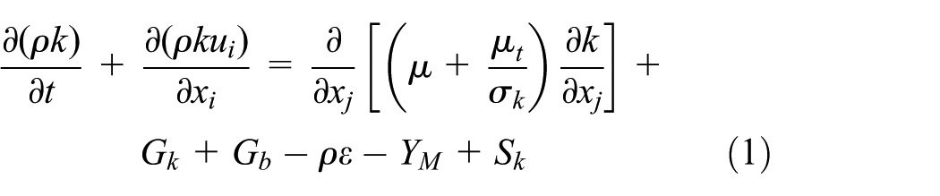
\frac{\partial (ρ k)}{\partial t} + \frac{\partial (ρ k u_{i})}{\partial x_{i}} = \frac{\partial}{\partial x_{j}} [(μ + \frac{μ_{t}}{σ_{k}}) \frac{\partial k}{\partial x_{j}}] + G_{k} + G_{b} - ρ ε - Y_{M} + S_{k}

(1)

where G_k is turbulent kinetic energy induced by average speed gradient, and G_b is turbulent kinetic energy induced by buoyancy effect. β is thermal expansion coefficient. Y_m is the effect of compressible turbulent pulsating expansion on the total dissipation rate. σ_k is the Prandtl number corresponding to kinetic energy. The default value in FLUENT is 1.0:

ε equation

\frac{\partial (ρ ε)}{\partial t} + \frac{\partial (ρ ε u_{i})}{\partial x_{i}} = \frac{\partial}{\partial x_{j}} [(μ + \frac{μ_{t}}{σ_{ε}}) \frac{\partial ε}{\partial x_{j}}] + C_{1 ε} \frac{ε}{k} (G_{k} + C_{3 ε} G_{b}) - C_{2 ε} ρ \frac{ε^{2}}{k} + S_{ε}

(2)

where C_1ε, C_2ε, and C_3ε are empirical constants. The default values in FLUENT are 1.44, 1.92, and 0.09, respectively.

Gasotron effect evaluation

To evaluate the rectifying effect of the gasotron on the fluid flow state, a method to estimate the stability of the flow velocity in the cross section of the pipeline is proposed. The simulation values in the cross section are compared with the theoretical calculation values.

Select a cross section of the pipeline, then determine the stability of the selected cross section based on its flow velocity profile. As shown Figure 1, to r₁ = r, r₂ = 2r, r₃ = 3r, r₄ = 4r, and r₅ = 5r radius concentric pipe cross section for each, where r = 0.2R, mark the simulating flow velocity of point each concentric circle intersecting with its own two mutually perpendicular diameters and the center of the circle as u_i, where i = 0, 1, 2, …, 20.

Figure 1.

Velocity sampling point in pipe cross section.

Define e_i as difference value between u_i and v_i, where v_i is theoretical calculation speed. v_in is the boundary speed in simulation. If for all i = 0, 1, 2, …, 20, the following formulas are satisfied, it can be determined that the medium velocity field on the cross section is in a stable state; otherwise, the cross section is considered to be a non-stable flow velocity cross section

e_{i} = | u_{i} - v_{i} | \leq Δ v

(3)

Δ v = \frac{1}{5} v_{in}

(4)

To quantify the rectification effect of the gasotron, an evaluation index L_min was introduced. The physical meaning of the index is the length of the straight pipe required to render the distortion flow into stable flow state after rectifying by the gasotron.^26–29

Basing on the stability estimation above, in the calculation of the rectification evaluation index L, the basic idea dichotomy is adopted. As shown in equations (5) and (6), by n times calculations, to identify whether the velocity of the cross section L_n is stable, for L_n satisfying equation (6) is supposed to be required result L_min

L_{n} = L_{n - 1} + \frac{1}{2} (L_{n - 2} - L_{n - 1}) (n = 2, 3, 4, \dots, n \geq 2)

(5)

| L_{n} - L_{n - 1} | \leq \frac{1}{2} R

(6)

The implementation is as follows:

Step 1. First of all, the section of the gasotron downstream length L₁ is arbitrarily selected to estimate the stability of the flow velocity. According to the simulation results, the velocity values of each point on the cross section of the pipe are obtained. The stability of the flow velocity at the cross section of L₁ is determined by equations (3) and (4). Then, find a cross section through which the flow velocity distribution is stable.

Step 2. Select the cross section of the gasotron downstream length L₂ = 0.5 L₁, repeat evaluation method of step 1 to find a cross section through which the flow velocity distribution is unstable.

Step 3. Select the cross section of the gasotron downstream length L₃ = L₂ + 0.5(L₁ – L₂), repeat evaluation method of step 1 to find a cross section through which the flow velocity distribution is stable and judge whether|L₃–L₂| satisfies for equation (6); if it does, end the calculation and take L₃ as L_min, if not, select the cross section of the gasotron downstream length L₄ = L₃ + (L₂ – L₃) and repeat the step above until finding a stable one and stratify equation (6).

Case study

Modeling

According to previous research, the header type DN300×2600 (P = 6.93 MPa) is selected to model for its high distortion to flow. Since plate gasotron is the widely used upstream ultrasonic flow meter, its modeling is employed in this study. As shown in Figure 2, the geometry model is set up by Pro/E. The origin of coordinates is at the intersection of the axis of the cross section of the header with the axis of the inlet straight section. The pipeline length from the entrance to the header (L₃) is set to three times the diameter (3D) of itself and the length from the header to the gasotron (L₁) is 6D. The metering length is 4D (i.e. length of the ultrasonic flow meter), and the distance between gasotron and the ultrasonic flow meter is 16D. The diameter of the metering pipe is DN150.

Figure 2.

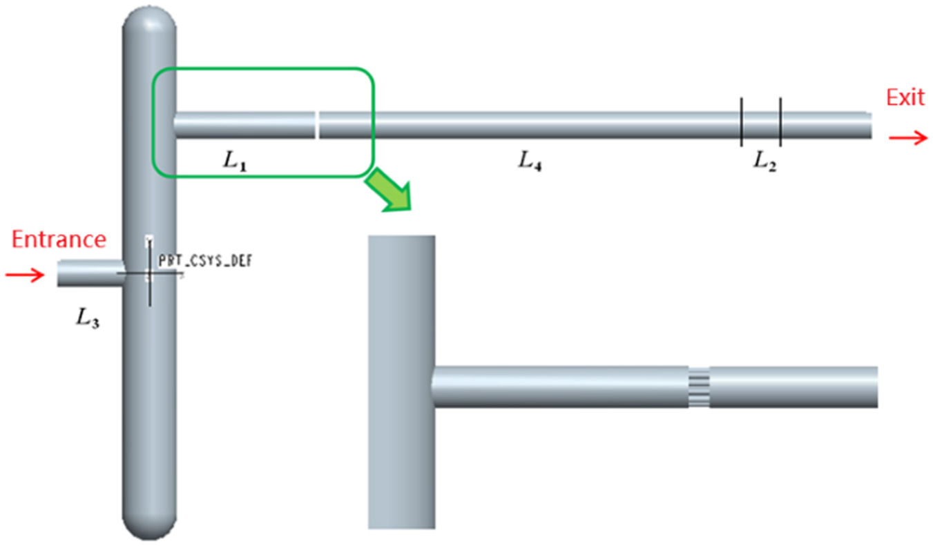
Geometry model of header and gasotron on metering segment.

The three-dimensional model was imported into ANSYS-ICEM to be meshed. The grid model is shown in Figure 3, with 624,255 grids totally for the calculation.

Figure 3.

Grid model of gasotron on metering segment.

The distribution of the internal gas flow field with different transmission flows Q and the length L of the downstream straight pipe section is analyzed. The header is DN300×2600 header, and the diameter of downstream pipe is DN150; three sets of simulating scenario results for comparative analysis: benchmark, header and 30D straight pipe, header and 19-hole plate gasotron, respectively.

Boundary conditions

The inlet boundary condition is “Velocity-inlet,” the exit boundary condition is “outflow,” and the wall boundary condition is default and “no slip” is employed. The operating temperature is 12°C, and the operating pressure is set as 0.8 MPa. The gas density is 0.68 kg/m³, and viscosity is 1.603 × 10⁻⁵ m²/s. The velocity of sound is 340.3 m/s. Table 1 shows the boundary conditions and flow velocity stability estimating value (i.e. Δv) in five different transmission conditions as follows.

Table 1.

Boundary conditions and flow velocity stability estimating value.

Sequence	Reynolds number $(Re)$	V (m/s)	Flow rate of verification, Q₁ (m³/h)	Δv (m/s)	P S
1	3.14e5	33.51	2131.91	6.702	Above the Q_t
2	1.29e5	13.77	875.73	2.754
3	8.22e4	8.78	558.86	1.756
4	3.17e4	3.39	215.68	0.678	Below the Q_t
5	5802	0.62	39.71	0.124	Below the Q_t

Results and discussion

The theoretical velocity of the sampling point in the cross section can be obtained (Figure 1), as shown in Table 2.

Table 2.

Theoretical velocity of the sampling point.

Boundary velocity, V (m/s)	V_max (m/s)	n	1.6.11.16r = 15 mm	2.7.12.17r = 30 mm	3.8.13.18r = 45 mm	4.9.14.19r = 60 mm	0r = 0 mm
0.62	0.789	5.28	0.756	0.716	0.663	0.581	0.62
3.39	4.109	6.57	3.972	3.802	3.574	3.216	3.39
8.78	10.391	7.3	10.078	9.689	9.165	8.335	8.78
13.77	16.2	7.66	15.735	15.155	14.374	13.130	13.77
33.51	39.424	8.35	38.384	37.084	35.327	32.513	33.51

The XY profile global velocity cloud around the gasotron (red area in Figure 4) in five transmission conditions are shown as below.

Figure 4.

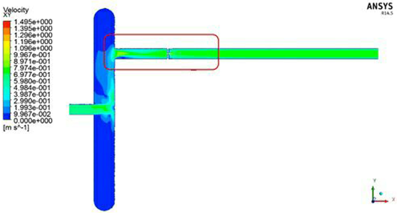
Contours of the XY velocity (Q = 39.71 m³/h).

Figure 5 indicates qualitatively that vortex and asymmetric flow distribution as a result of distortion by header developing into stable flow state soon after rectified by gasotron. It represents the XY profile global velocity cloud when the flow is 39.71, 215.71, 558.86, 875.73, and 2131.91 m³/h, respectively.

Figure 5.

Contours of the XY velocity with different flow rates: (a) Q = 39.71 m³/h, (b) Q = 215.68 m³/h, (c) Q = 558.86 m³/h, (d) Q = 875.73 m³/h, and (e) Q = 2131.91 m³/h.

Figure 6 shows the velocity distributions across the cross section of different downstream lengths when the flow rate is 875.73 m³/h.

Figure 6.

Velocity distributions across the cross section of different downstream lengths (Q = 875.73 m³/h).

It can be seen that the flow velocity profile represents relatively uniform concentric circles distribution at L = 10D. Read the simulating velocity u_i at each sample point marked in Figure 1. According to Table 2 and Figure 6, for each i = 0∼20, equation (3) is established, where Δv = 0.2V_in = 2.754 m/s. It does not satisfy ∣L_n–L_n_–1∣ ≤ 0.5. Therefore, select L₂ = 0.5 L₁ and repeat the steps before. If the velocity of cross section at L = 5D is unstable, then increase the L. We can obtain L_n = 6.719D and L_n_– 1 = 6.563D satisfying above requirements. Therefore L = 6.719D can be determined as L_min when Q = 875 .73 m³/h. The rectifying effect of rest of other four transmission conditions can be figured out by above steps, as shown in Table 3.

Table 3.

L_min in five transmission conditions.

Sequence	Reynolds number (Re)	V (m/s)	Δv (m/s)	L (nD)	P S
1	3.14e5	33.51	6.702	7.5D	Above the Q_t
2	1.29e5	13.77	2.754	6.719D
3	8.22e4	8.78	1.756	6.68D
4	3.17e4	3.39	0.678	6.641D	Below the Q_t
5	5802	0.62	0.124	6.563D	Below the Q_t

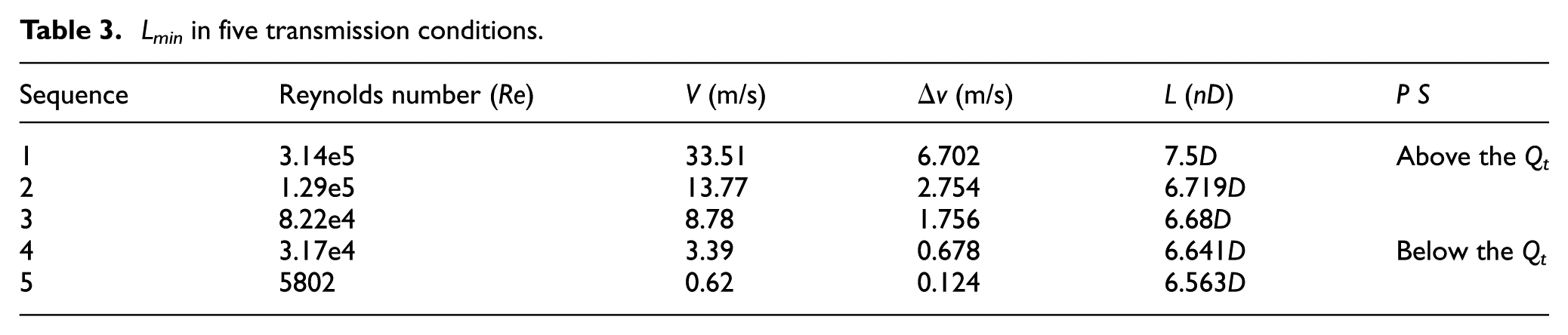
It indicated that the installation of the flow meter at the downstream L = 8D of the gasotron can ensure the flow field of the gas downstream header and gasotron stable when the ultrasonic flow meter working in five groups of transmission conditions, while the required straight pipe length is 27D for stability of flow state and indication errors with no gasotron at the pipe with header.

According to simulating results in three installation conditions, indication errors can be obtained. As previous study shows that when there is a header upstream located on pipeline, 27D straight pipe section at upstream of pipeline is supposed to be ensured to render the gas flow into uniform stable state.^30,31 Therefore, Figure 7 shows the indication errors in header with 27D straight pipeline, benchmark, and header and gasotron with 8D straight pipeline, such three installation conditions.

Figure 7.

The trends of indication errors in different installation conditions.

In benchmark, gas enters the measuring pipe section, of which diameter is DN150, through the header, the length of straight pipeline at upstream of ultrasonic flow meter is 160D, a plate gasotron is installed at 10D upstream of ultrasonic flow meter, and the downstream length of gasotron is 20D. The ultrasonic flow meter adopted for measurement is Daniel SeniorSonic™, which flange with measuring pipe section. As we can see when the gas flow state reaches a steady state, the indication errors range of the flow value on each cross section is 0.32%–1.47%. When there is a header and gasotron on the pipeline, the trends of indication errors and its values are basically similar. The offset range is between 0.03% and 0.2%. The detail information is shown in Table 4; when the flow rate is below Q_t, the simulation errors of case 1 exceeds ±1%, which does not meet the minimum performance requirements of the ultrasonic flow meter. In the other two installation conditions, the errors below the Q_t is within ±1%, the mean values are 0.75% and 0.82%, while the indication errors above the Q_t are both within ±0.5%, the mean values were 0.32% and 0.39%, respectively. It means the installation of gasotron at D > 8D upstream the ultrasonic flow meter could improve the metering accuracy well.

Table 4.

Indication errors in different installation conditions.

Sequence	Reynolds number (Re)	Flow rate, Q (m³/h)	Header and 27D straight pipeline		Benchmark (150D straight pipeline)		Header and gasotron with 8D straight pipeline		P S
Sequence	Reynolds number (Re)	Flow rate, Q (m³/h)	Simulation rate flow	Indication errors	Experimental estimation	Indication errors	Simulation rate flow	Indication errors	P S
1	5802	39.71	40.29	1.47	40.01	0.75	40.09	0.95	Below the Q_t
2	31,700	215.68	217.45	0.82	217.28	0.74	217.15	0.68	Below the Q_t
3	82,200	558.86	562.83	0.71	561.1	0.40	561.71	0.51	Above the Q_t
4	129,000	875.73	880.81	0.58	877.57	0.21	878.8	0.35
5	314,000	2131.91	2142.14	0.48	2139.37	0.35	2138.73	0.32

According to JJG 1030-2009 “Ultrasonic Flowmeter” verification regulations, since the installation of gasotron at D > 8D upstream of the ultrasonic flow meter, the flow state has been restored to the performance range that the flow meter can compensate.²

Conclusion

This study systematically identified the evaluation method of rectification effect of gasotron and its implementation steps. The CFD method was used to simulate the geometric model of the header and plate gasotron in the upstream straight section of the flow meter and obtained quantitatively the L_min in different transmission conditions. When length of downstream gasotron straight pipeline L > 8D, the flow fields can all reach stable state at given transmission flow rate. Comparing indication errors in three different installation conditions—pipeline with header, benchmark, and pipeline with header and gasotron—on which when there is a header and gasotron upstream of the ultrasonic flow meter, the changing range of indication error basically being accordance with ones in benchmark, within 0.03%–0.2%, while the other two conditions the indication error both within ±0.5%, all satisfy the relevant standards stipulated ultrasonic flow meter minimum performance requirements. The feasibility of gasotron was validated.

Footnotes

Handling Editor: Hongfang Lu

Declaration of conflicting interests

The author(s) declared no potential conflicts of interest with respect to the research, authorship, and/or publication of this article.

Funding

The author(s) received no financial support for the research, authorship, and/or publication of this article.

ORCID iD

Shanbi Peng

References

Bao

Research on the main factors causing error on measurement of ultrasonic gas flowmeters: theory and applications. PhD Thesis, Zhejiang University, Hangzhou, China, 2004, pp.29–31.

Liu

Yang

Optimal energy consumption analysis of natural gas pipeline. Sci World J 2014; 2014: 506138.

Mattingly

Yeh

TT.

Effect s of pipe elbows and tube bundles on selected types of flowmeters. Flow Meas Instrum 1991; 2: 4–13.

Morrow

Park

Mckee

RJ.

Determination of installation effects for a 100 mm orifice meter using a sliding vane technique. Flow Meas Instrum 1991; 2: 14–20.

Laws

Ouazanne

AK.

Compact installations for differential flowmeters. Flow Meas Instrum 1994; 5: 79–85.

Morrison

DeOtte

R Jr

Beam

et al . Installation effects upon orifice flowmeters. Flow Meas Instrum 1992; 3: 89–93.

Morrison

Panak

DeOtte

RE.

Numerical study of the effects of upstream flow condition upon orifice flow meter performance. J Offshore Mech Arct 1993; 115: 213–218.

Morrison

DeOtte

Moen

et al . Beta ratio, swirl and Reynolds number dependence of wall pressure in orifice flowmeters. Flow Meas Instrum 1990; 1: 269–277.

Morrison

Hauglie

DeOtte

Jr.

Beta ratio, axisymmetric flow distortion and swirl effects upon orifice flow meters. Flow Meas Instrum 1995; 6: 207–216.

10.

Lee

ZL.

Numerical simulation of flows in the flow rate measurement section with a rectifier in a natural gas pipe. J Petrochem Univ 2008; 21: 78–86.

11.

XX.

Experimental study on the flow conditioning of the water-pipe network installed with flow conditioner. Master’s Thesis, Xi’an University of Architecture and Technology, Xi’an, China, 2017.

12.

Liu

Huang

QW.

Evaluation method of effect of rectifier based on CFD. CN 102750426, 2012.

13.

Smith

DJM.

The effects of flow straighteners on orifice plates in good flow conditions, Commisson of the European Commission, 1996.

14.

Brennan

Sindt

Lewis

et al . Choosing flow conditioners and their location for orifice flow measurement. Flow Meas Instrum 1991; 2: 40–44.

15.

Spearman

Sattary

Reader-Harris

MJ.

A study of flow through a perforated-plate/orifice-meter package in two different pipe configurations using laser Doppler velocimetry. Flow Meas Instrum 1991; 2: 83–88.

16.

Spearman

Sattary

Reader-Harris

MJ.

Comparison of velocity and turbulence profiles downstream of perforated plate flow conditioners. Flow Meas Instrum 1996; 7: 181–199.

17.

Wendt

Mickan

Kramer

et al . Systematic investigation of pipe flows and installation effects using laser Doppler anemometry—part I. Profile measurements downstream of several pipe configurations and flow conditioners. Flow Meas Instrum 1996; 7: 141–149.

18.

Mickan

Wendt

Kramer

et al . Systematic investigation of pipe flows and installation effects using laser Doppler anemometry—part II. The effect of disturbed flow profiles on turbine gas meters—a describing empirical model. Flow Meas Instrum 1996; 7: 151–160.

19.

Wei

Kalkühler

Merzkirch

et al . Velocity and turbulence measurements downstream of flow conditioners. Flow Meas Instrum 2003; 14: 249–260.

20.

Essel

Tachie

Agelin-Chaab

et al . Particle image velocimetry measurements in curved turbulent jets produced from a slot diffuser. Exp Therm Fluid Sci 2013; 49: 169–184.

21.

Liu

Tan

Peng

SB.

A CFD simulation for the ultrasonic flow meter with a header. Teh Vjesn 2017; 24: 1797–1801.

22.

Liu

Wen

Peng

et al . A study of the numerical simulation of water hammer with column separation and cavity collapse in pipelines. Adv Mech Eng 2017; 9: 1–13.

23.

Liu

Yan

Peng

et al . Noise silencing technology for manifold flow noise based on ANSYS fluent. J Nat Gas Sci Eng 2016; 29: 322–328.

24.

Liu

Yan

et al . Large eddy simulation and FW-H acoustic analogy of flow-induced noise in elbow pipe. J Comput Theor Nanos 2016; 12: 2866–2873.

25.

Laws

EM.

Flow conditioning: a new development. Flow Meas Instrum 1990; 1: 165–170.

26.

Chen

ZS.

Model test and numerical simulation about flexible pipe systems subject to vortex-induced vibration. Master’s Thesis, Ocean University of China, Qingdao, China, 2009.

27.

Huang

QW.

Characteristics simulation and optimization on the flow field of U-channel ultrasonic flowmeter with a flow conditioner. Master’s Thesis, South China University of Technology, Chengdu, China, 2015.

28.

Research on gas flowmeter and rectifier application. Master’s Thesis, Southwest Petroleum University, Chengdu, China, 2011.

29.

Kai

Design and research of ultrasonic flow meter based on time difference method. Master’s Thesis, South China University of Technology, Guangzhou, China, 2013.

30.

Huan

Numerical simulation of manifold’s effect on the velocity field of gas pipeline downstream. Contemp Chem Ind 2015; 44: 215–220.

31.

Peng

Liu

Xian

et al . Dynamic simulation of an underground gas storage injection-production network. J Environ Biol 2015; 36: 799–806.

Performance optimization of ultrasonic flow meter based on computational fluid dynamics

Abstract

Keywords

Introduction

Methods

Mathematic model

Gasotron effect evaluation

Case study

Modeling

Boundary conditions

Results and discussion

Conclusion

Footnotes

Declaration of conflicting interests

Funding

ORCID iD

References