
Abstract
The swirl meter is one of the gas flow meters used in the industry. Its advantages are as follows: a strong signal level, easy maintenance, and stable performance. Hence, it has become widely accepted for natural gas metering. In this study, the numerical computation of the three-dimensional unsteady flow in a swirl meter was conducted using the renormalization group k–ε turbulence model and SIMPLE algorithm. The internal flow fields were analyzed in detail, wherein the velocity and pressure distributions were discussed under six flow rates (6, 15, 25, 40, 70, and 100 m3/h) and three swirl cone angles (11°, 20°, and 30°). The obtained results are reported and discussed as follows: the stable performance of the swirl meter was due to its capacity to maintain its internal characteristics over a large flow range. Also, it was detected that though the pressure decrease was gradual on the wall, an opposite tendency was shown at the center. On the other hand, the swirler structure was crucial to the metering capacity of the swirl meter, and the swirler cone angle influenced the pressure and velocity.
Introduction
Gas flow meters are the main instruments used for flow measurement; the accuracy of the flow rate determines the safe operation of the entire processing system. Based on the unique fluid oscillating phenomenon, flow rates are measured by the swirl meter by processing the oscillating frequency that is proportional to the flow rate. Among dozens of flow meters invented for industrial applications, the swirl meter stands out on the merits of its strong signal level, wide range, and stable performance. Hence, it has been widely used in the natural gas industry.
The first swirl meter was invented in the 1960s by Fischer & Porter Co based on the American standard; Dijstelbergen 1 elaborated on the operating principle in 1970 and pointed out that the swirling jet in the swirl meter did not take a fixed position at the downstream of the throat, but rotated around the axis of the measuring tube. The author compared this phenomenon to that of a spinning top where the axis of the top rotated around a line perpendicular to the surface and makes precession motion. In 1979, Lee et al. 2 established a more precise and concrete physical model using high-speed photography techniques. Four stages of vortex flow, namely, the formation, development, precession, and breakdown, were discovered in the swirl meter. Lee et al. 2 also proposed two basic formulas: one formula revealed the relationship between the vortex and structure parameter, while the other formula expressed the characteristics of the vortex precession. The development of sensors advanced the technological breakthrough of swirl meters in the 1990s which was due to the capacity to process the differential pressure signal detected by the piezoelectric pressure sensors. Thus, the signal strength, measuring range, anti-interference property, and performance were significantly improved. 3
In the past decades, the computational fluid dynamics technique was widely used for the flow field analysis of the flow meter. Venugopal et al. 4 conducted experimental and numerical investigations for the vortex flow meter with various bluff body shapes and discovered that the k–ε renormalization group (RNG) model’s Strouhal number prediction was closer to experimental results than that of k–ε Realizable and k–ε standard models. Hollingshead et al. 5 studied the Venturi, V-cone, and wedge flow meters at low Reynolds numbers and discovered that the discharge coefficients’ rate of decrease was higher with a decreasing Reynolds number. Borkar et al. 6 explored a novel pressure-averaging technique to enhance the performance of the cone flow meter for measuring flow disturbance. Singh and Tharakan 7 simulated the flow in the single-hole and multi-hole orifice meters and discovered that early reattachment of flow in the multi-hole orifice meter could reduce the pressure loss. By utilizing the torque balance theory, Saboohi et al. applied numerical methods to obtain the internal flow field of the turbine flow meter and conducted a detailed analysis of the pressure and velocity inside. They pointed out that by considering bearings drag torque, the simulative results improved and got closer to experimental data. 8 Moosa and Hekmat 9 numerically investigated the turbulence characteristics of orifice flow meters, and then they discovered that multi-hole orifices had a higher discharge coefficient and less sensitivity to upstream disturbances. Zheng et al. 10 simulated flow in the ultrasonic flow meter for two typical transducer installations and pointed out that the negative velocities generated at protrusion and recess locations were the core factors causing the negative measurement errors.
Attempts are also being made to simulate the internal flow of swirl meter. Fu et al. utilized the large eddy simulation method to investigate the vortex precession and the hydrodynamic oscillation mechanism of the swirl meter. The results show that the pressures at axisymmetric positions fluctuated with the same frequency and intensity but with a 180° phase shift. 11 Liu et al. 12 investigated the effect of the sleeve valve on the performance of the swirl meter and discovered that the metrological performance was easily affected by the upstream throttling effect. Cui et al. numerically studied the effect of the geometric construction on the flow field distributions of the swirl meter. The results show that with increasing swirler helix angle, the pressure loss and meter factor decrease linearly. Therefore, increasing the lead of the swirler and the throat diameter could result in better pressure loss and performance.13,14
In our previous research, we analyzed the flow fields and studied the influence of measuring tube structure and found throat diameter played an important role in determining the precession frequency.15–18 Moreover, a detailed flow analysis of swirl meter performance was performed by processing physical quantities into time-averaged ones, the focus was about the basic characteristics of pressure and velocity at different regions. 19 On the foundation of former investigation, in present study, the internal flow fields were also processed into time-averaged results that provided a new perspective to understand the distribution characteristics and help grasp the mechanism behind the swirl meter’s capacity to maintain stability over a large flow range. The effect of the swirler cone angle on internal flow fields and the overall metrological performance were investigated in detail.
The paper is organized as follows: First, the research model of swirl meter including three different structures and the numerical method is introduced. Then, the numerical results of pressure and velocity at cross sections from inlet to outlet under different flow rates are discussed. Next, the comparison of flow fields with different swirlers is performed and analyzed in detail. Finally, experiment is conducted to verify the simulation results and show good agreement.
Numerical modeling
A swirl meter consists of a measuring tube (Venturi-like tube), swirler, de-swirler, sensors, signal processing module, display, and so on. The measuring tube consists of a convergent section, throat, divergent section, and straight tube downstream, while the swirler consists of six helical blades and a shaft, as shown in Figure 1. Notably, the vortex, which is usually formed after the fluid passes through the swirler, plays a dominant role in determining the flow in the swirl meter. Therefore, we focused on the effects of the swirler’s structure parameters on the swirl meter performance, and the cone angle is studied in detail in this paper.
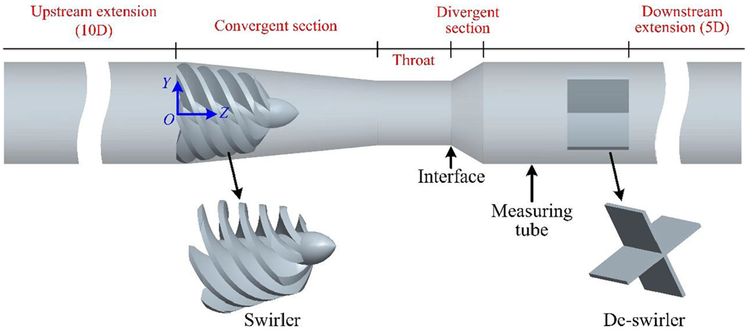
Computational domain of the swirl meter.
A DN50 swirl meter was taken as the research model; the three-dimensional structure was modeled using the commercial software (Pro/E). The cone angle of the prototype swirler was 20°, and the angle of convergence of the convergent section in the measuring tube was 11° when the minimal cone angle was 11°, and a larger cone angle of 30° was taken. The swirler is shown in Figure 2. Three swirl meters with cone angles of 11°, 20°, and 30° were built. To assure a fully developed flow during simulation, a 10-diameter (10D) length upstream pipe and 5-diameter (5D) length downstream pipe were set as extensions.
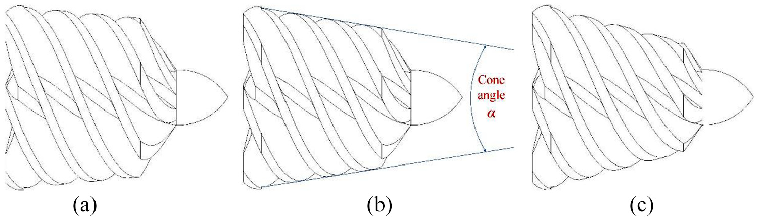
The swirler with different cone angles: (a) α = 11°, (b) α = 20°, and (c) α = 30°.
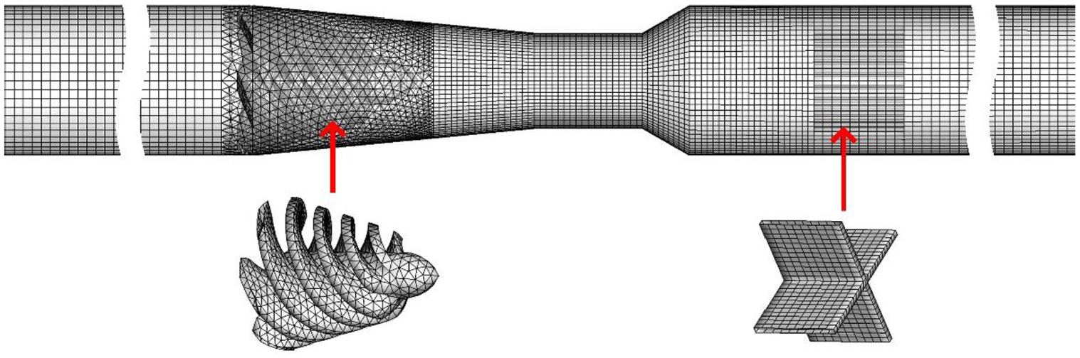
The numerical meshes were generated using the Gambit software and shown in Figure 3. During meshing, the computational domain was separated into upstream extension, swirler region, throat, and divergent section, de-swirler section, and downstream extension. Given that the swirler has a complicated structure with spiral blades, we adopted unstructured tetrahedral meshes with strong adaptability to capture a precise structure. For the other regions, hexahedral structured meshes with high quality were adopted to reduce the total number of spiral blades and improve computing efficiency. For the core regions between the swirler and de-swirler, the local refinement technique was adopted to obtain a better-detailed flow field.
Computational meshes.
The flow fields of prototype swirl meter (swirler cone angle was 20°) with different mesh numbers were analyzed, mean pressure at the interface between throat and divergent section (using piezoelectric sensor, the vortex precession signal was detected at this area in the industrial application; location is shown in Figure 1) was taken to make the comparison. As shown in Figure 4, the result differences were small when the number was over 3 million; therefore, the mesh of 3.8 million was adopted (it showed a slight difference in different swirlers). The y+ was also under consideration during mesh generation, the maximum value was smaller than 72 for all flow conditions, and it meant the meshes were capable to obtain an accurate simulation result.
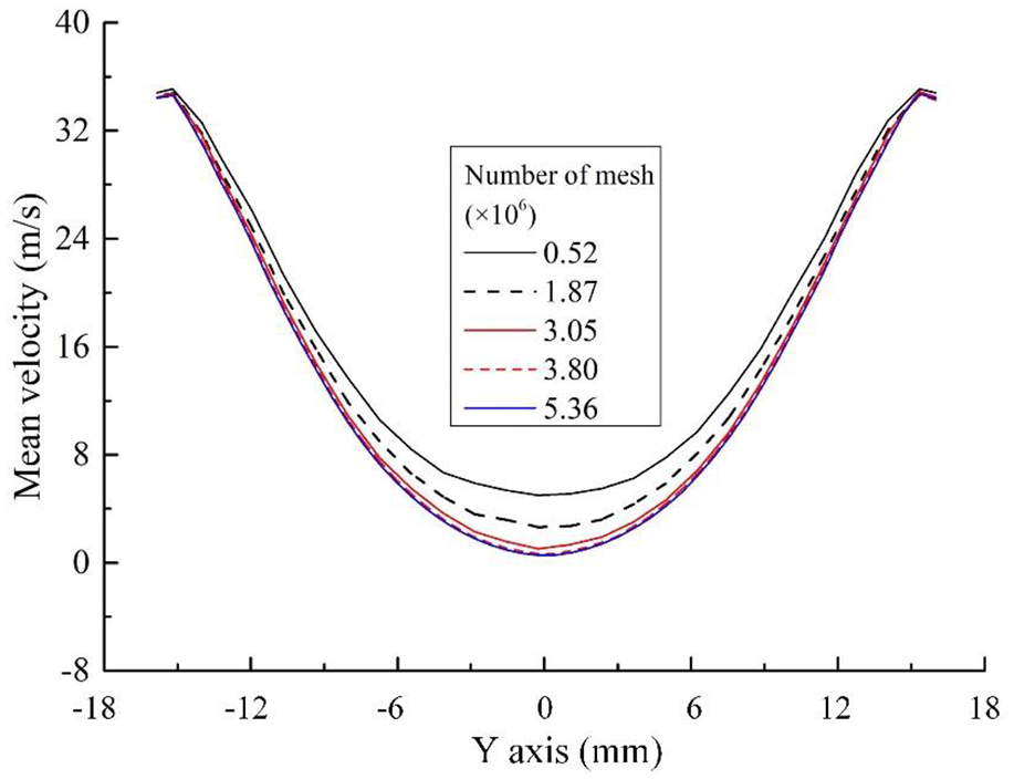
Verification of grid independence (mean velocity at interface).
The numerical simulations for different swirl meters were implemented in Fluent 16.0. In the course of computation, the RNG k–ε turbulent model and SIMPLE (Semi-Implicit Method for Pressure Linked Equations) algorithm were adopted to solve the governing equations. 20 The velocity at the inlet was specified, and a pressure of 0 Pa was given at the outlet of the computational domain. The standard wall function was adopted to solve the flow near the solid wall. The monitoring point was set at the end of the throat, which was the same location the piezoelectric crystal sensor was assembled. This was to capture a precise precession frequency in the swirl meter. The pressure showed regular variation; hence, this computation was convergent.
Based on the national standard of the People’s Republic of China (GB/T 36241-2018, vortex precession flow meter for gas), in this study, the swirl meter was investigated under seven flow conditions including the Qmin, 0.1Qmax, 0.15 Qmax, 0.25 Qmax, 0.4 Qmax, 0.7 Qmax, and Qmax. The rated flow range of our proposed model is 6–100 m3/h. That is, flow rates of 6, 10, 15, 25, 40, 70, and 100 m3/h were numerically simulated and tested. The calculation was accomplished using the Dell Precision T5610 workstation, the CPU was Xeon E5-2650, and the RAM was 64GB.
Numerical result analysis
The mean pressures and axial velocities along the flow directions at 6 m3/h (0.85 m/s), 40 m3/h (5.66 m/s), and 100 m3/h (14.15 m/s) are presented in Figures 5 and 6. As shown in the figures, the mean axial velocity is symmetrically distributed from the inlet to the outlet of the swirl meter. Due to the decreasing flow area in the convergent section, the fluid flow gains acceleration, which ensures the formation of the vortex and final precession motion. A clear reflux zone was discovered in the divergent section. Hence, the rapid expansion of the structure results in the generation of flow that occupies half of the passage. Meanwhile, the fluid in the swirl meter mainly flows close to the measuring tube wall due to the lower velocity at the center of the passage. Therefore, a local high-velocity zone was discovered at the junction of the throat and divergent section due to the reflux.
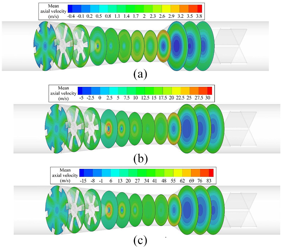
Mean axial velocity: (a) Q = 6 m3/h, (b) Q = 40 m3/h, and (c) Q = 100 m3/h.
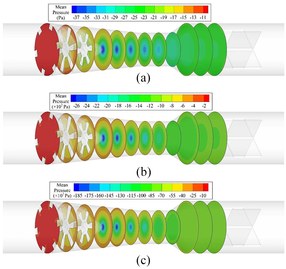
Mean pressure distribution: (a) Q = 6 m3/h, (b) Q = 40 m3/h, and (c) Q = 100 m3/h.
Based on the previous research,15,16 the fluid in the swirl meter in the three-dimensional simulation has an unsteady flow and is more complex when compared with differential meters like the orifice flow meter and wafer cone flow meter. Hence, it is difficult to study the differences under various incoming flow conditions and different structures. Therefore, to achieve an intuitive comparison on the parameters, the time-averaged data were applied to analyze the overall distribution in the swirl meter over a wide range for different swirlers.
Figure 5 shows a comparison of the internal average axial velocity at different flow rates. It presents accurate characteristics of the overall flow fields and the return flow area in the flow meter. In the flow channel formed by the spiral blades of the swirler, the fluid medium (gas, steam, etc., air was taken during present simulation) obtains additional tangential velocity in addition to the axial flow acceleration, thereby forming a vortex flow at the swirler outlet. A high-velocity zone was found in the area close to the cone of swirl shaft. Of the possible fluid media which include gas, steam, and so on, the air was chosen in our simulation. Meanwhile, the velocity was low and the reflux was at the tip of the cone. Huge reflux was present at the divergent section while the velocity close to the wall at the end of the throat was relatively higher.
At different flows, the pressure was uniformly and symmetrically distributed. The decreasing pressure and other variations were consistent in swirler region. After forming the vortex at the downstream of the swirler, two opposite trends appeared at the passage center and tube wall. The minimal pressure was found at the center of the passage. Also, at the exit of the swirler, the pressure at the passage center gradually increased as the flow developed downstream. While for the tube wall and its vicinity, the pressure kept decreasing and then stabilized at the downstream of the divergent section.
The overall distributions for the velocity at different flow conditions were the same, and the same trend was observed for other distributions. This proves that the internal characteristics in the swirl meter remain constant over a wide range and guarantee a stable performance in measurement.
The pressure difference was clear at the inlet and outlet of the swirl meter, which, in this case, stands for a noticeable energy loss during flow measurement. The loss was produced in two main processes, the acceleration of flow in the swirler and the vortex precession at the throat. Considering that the formation of vortex was determined by the tube structure and swirler, the swirler played a dominant role in the entire flow and flow measurement in the swirl meter. The influence of the swirler cone angle was analyzed in detail in the next section.
Effect of the swirler cone angle on the performance of the swirl meter
In the swirl meter, flow acceleration is the basis of forming a strong vortex and the main process occurs in the swirler. The velocity at midsection is shown in Figure 7 (Q = 40 m3/h). It is presented in the form of velocity increments to reveal the basic velocity distribution characteristics where V stands for the local velocity in the swirl meter and Vin is the inlet velocity. As shown in the figure, the fluid gains acceleration since it flows into the swirler. The maximal velocity is at the vertex region of the swirler and the increment could go as high as eight times of the inlet velocity. Although the flow path continues to decrease, the overall velocity decreased after vortex was formed at the swirler exit. The vortex developed at the downstream of the convergent section and throat region; meanwhile, velocity kept decreasing and the vortex precession motion seemed not to influence on the overall decline in velocity. The main influence of the swirler cone angle on the velocity was at the swirler region. Thus, for a smaller cone angle, the fluid obtained a higher acceleration.
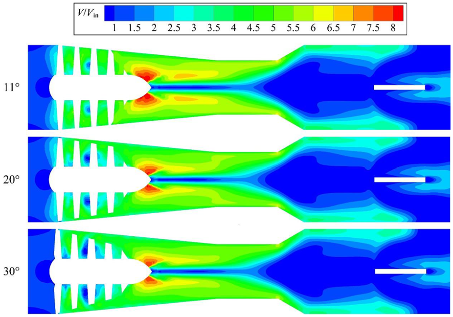
Velocity at midsection with different cone angles.
As shown in Figure 8, the change in pressure was opposite to the velocity change. After entering the swirler, due to the drastic change of the flow channel structure, the fluid hit the surface of the swirler blades. As the flow velocity increased, a clear pressure drop was observed, and the pressure near the tube wall was higher in the same section. For different cone angles, the distributions were the same, the pressure decreased gradually on the wall, and there was an opposite trend at the passage center. The pressure of the cone angle at 11° was lower, but for the other two swirlers, the difference was unclear.
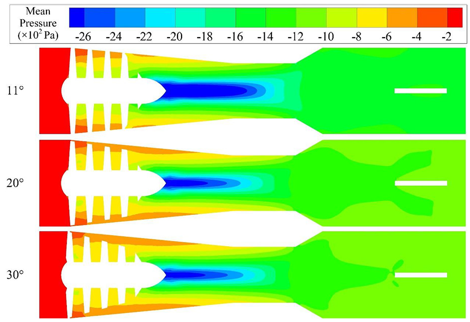
Pressure at midsection for different cone angles.
The velocity and pressure profiles from the inlet to the outlet are shown in Figure 9 (the mean data at cross-sections). The overall distribution law for the pressure was relatively simple; also, there were two main processes involved: one was the process of continuous decline from the beginning of the swirler’s entrance to the end of the throat and the other was the process that entailed a gradual increment in the expansion section. The latter process was a result of the rapid decrease of the pressure inside the swirler and the invariant conditions in the three flow meters. This process was mainly caused by the energy loss accompanying the high-speed impact of the fluid on the blade surface; thereby, the pressure kept decreasing after flowing out of the swirler at a slower rate. At the end of the throat, the pressure was at its lowest. The influence of the cone angle on the pressure distribution was mainly concentrated in the convergent section. The difference between the cone angles 20° and 30° was the same, while a much higher pressure drop was found at 11°. In the throat and divergent sections, the variation was the same for the three cone angles.
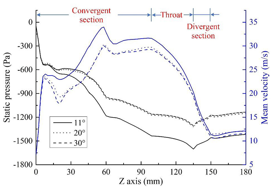
Pressure and velocity distributions along the flow direction.
The distribution of the velocity was more complicated. At the inlet region of the swirler, a sudden increase in velocity occurs during the rapid drop of pressure. Based on the velocity profile for the entire acceleration process, over 60% of the increment was completed at the beginning of flow in the swirl meter. As the fluid flowed through the blades, backflow occurred, causing a decrease in the velocity. After that, acceleration gain occurred with the contraction of the flow passage. As vortex formed at the outlet of swirler and backflow occurred at the center region, the flow was further decreased. At the other parts of the convergent section, velocity increased gradually. The third time with an observed rapid drop in velocity was at the throat and divergent section. After that, flow becomes stable downstream. The overall velocity in the swirl meter was larger for the cone angle of 11°, and the maximal value was about 10% higher than the other two structures. Unlike for pressure, the influence of the cone angle on velocity vanished at the end of the throat.
The centerline pressure profile under different cone angles is shown in Figure 10. As shown, the overall trend was opposite to the results in Figure 9, wherein the pressure increased gradually from the exit of the swirler and started to maintain stable values in the divergent section. The pressure change on the centerline was gentle; there was only a simple incremental process. No obvious difference was found between the cone angles of 20° and 30° which was due to the higher drop after passing the swirler. The overall pressure was lower for the cone angle of 11°. From the observed profile, the swirler cone angle had no direct impact on the centerline pressure distribution.
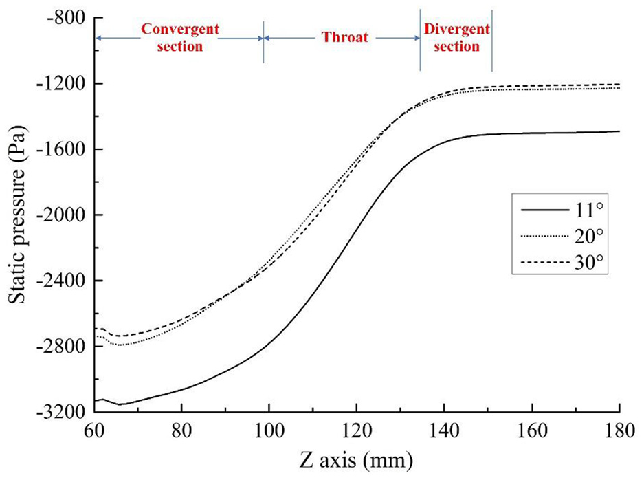
Pressure profiles on the centerline.
The velocity and axial velocity on the centerline are shown in Figures 11 and 12. Due to the reflux, the velocity at the swirler outlet had complicated readings. At the throat region, the velocity increased and reached the maximal. It then began to descend rapidly, reaching a minimum at the end of the throat. In the divergent section, the velocity started to increase again. The velocity at different cone angle conditions showed the same tendency. While the 20° cone angle had a higher velocity at the throat, for the 11° cone angle, it was smallest. Based on the results of Figures 8 and 10, the cone angle had different effects on centerline and overall velocity.
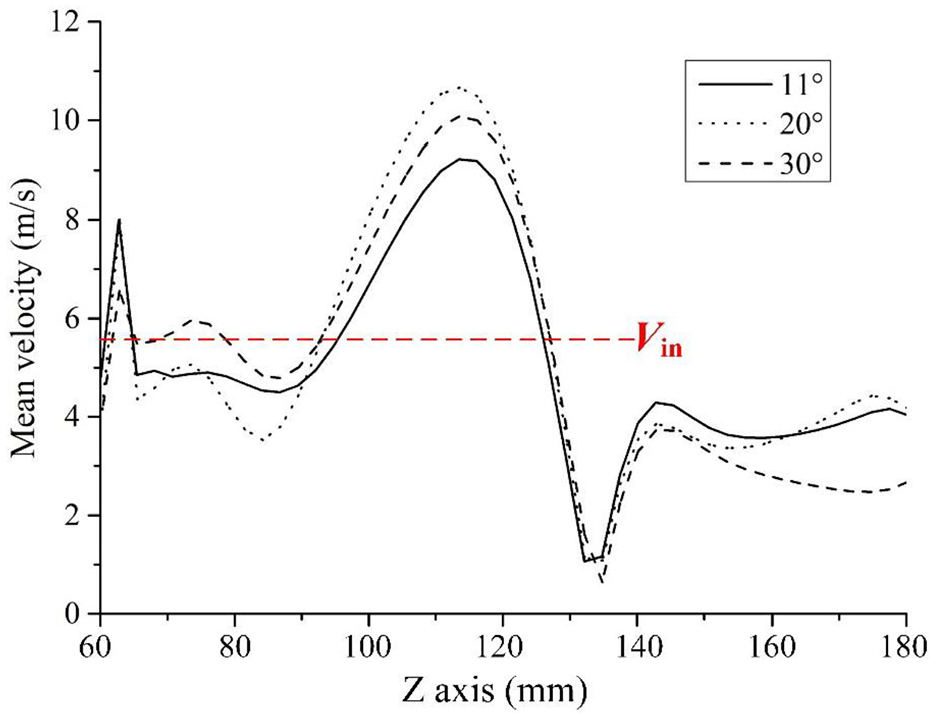
Velocity on the centerline.
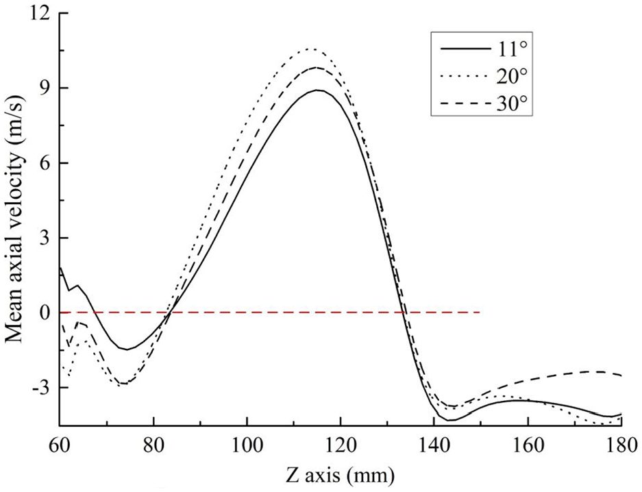
Axial velocity on the centerline.
The distribution of the axial velocity was similar to the velocity. Two reflux areas were found at the swirler outlet, divergent section, and its downstream, and the cone angle did not influence these events. In comparison with the velocity distribution, the axial velocity displayed no obvious speed recovery downstream of the throat. Moreover, the decreasing velocity occurrences were limited to the throat area, while the axial velocity kept decreasing at the divergent section.
The pressure at different cross-sections from the swirler outlet to the end of the throat is shown in Figure 13 (e.g. Z60 stands for the cross-section at Z = 60 mm). At the outlet of the swirler, the pressure is extremely lower in the center, while it is relatively high on the wall (it gradually increases from the center toward the wall). With this skewed distribution, a huge pressure difference was produced, thus creating a strong vortex flow. Given that the flow develops toward downstream, the pressure at the center and wall present opposite tendencies. The pressure on the wall showed the same variation law with the overall distribution analyzed in Figure 8 where it kept decreasing, thereby resulting in the minimization of the pressure difference in the same cross-section. In the course of transit analyzation, the pressure fluctuation was intense at the end of the throat where vortex precession was the strongest. The pressure distributions and the variation inside the swirl meters were the same for different swirlers; however, the difference in the values was significant. This was more pronounced when the cone angle decreased to 11°. Otherwise, the pressure on the wall and at the center both increased with increasing cone angle.
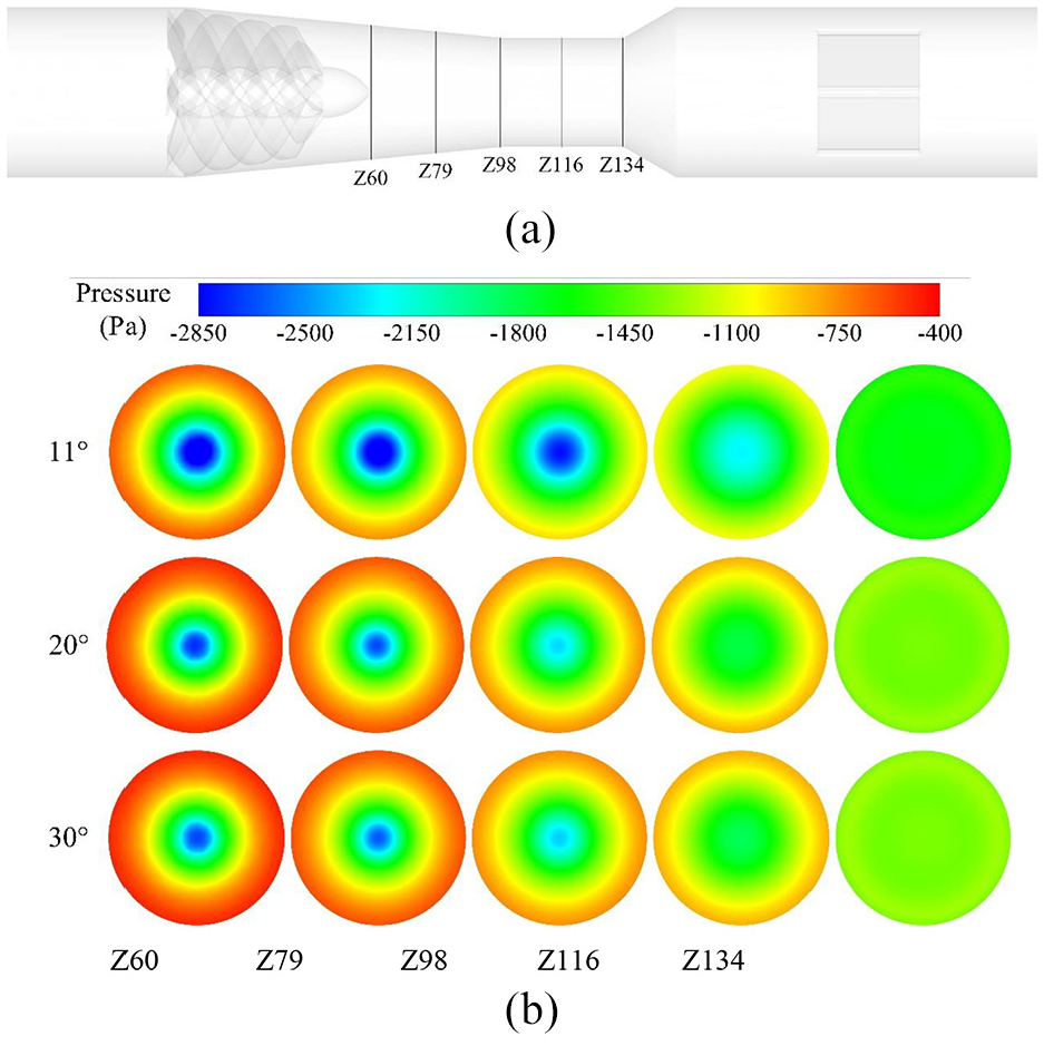
Pressure distributions for different cone angles: (a) location of cross-sections and (b) pressure at cross-sections.
The detailed pressure and velocity profiles at the swirler outlet (Z60), junction of the convergent section, throat (Z98), and the throat end (Z134) are shown in Figure 14. There are significant differences in the velocity distribution at different regions. At the swirler outlet, a large velocity gradient was observed near the center; however, a linear decrease was observed at the wall. Close to the tube wall region, the velocity was higher when the cone angle was 11°. At the junction of the convergent section and throat, the minimal velocity was the same as that at the swirler outlet. From the center to the wall, three processes (increasing, steady, and decreasing levels in the curve) were observed. The velocity was also higher when the cone angle was 11°. The velocity at the end of the throat was more regular; the minimum (close to zero) was at the center. From the center to the tube wall, the velocity increase was steady. Thus, the difference between the three swirlers was relatively small, indicating that the cone angle had a small effect on the velocity in this region.
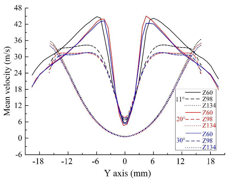
Velocity profiles in the cross-sections.
In comparison with the velocity, the variation of the pressure was simpler. As shown in Figure 15, the pressure at the end of the throat remained constant from the center to the wall. However, it was lower at the cone angle of 11°, which was the same for the other structures. The pressure showed the same tendency at the other regions, that is, it kept increasing from the center to the wall, and it was always lower for cone angle of 11°.
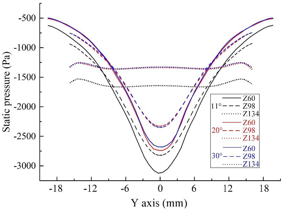
Pressure profiles in the cross-sections.
Experiment results and validation
Experiment plays an important role in the validation of the numerical results,21–24 the swirl meters were tested using the standard sonic nozzle gas flow device, as shown in Figure 16. The device has an error of 0.2%. This experiment aims to obtain the meter factor K of the swirl meter; the definition is as follows
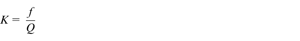
where Q is the flow rate and f is the corresponding vortex precession frequency. The flow rate Q was measured by the sonic nozzle and f was detected by the piezoelectric sensors in the swirl meter; all signals were transmitted to a computer via the RS485 communication port. The meter factor K is a structure factor which depends on the structure of the swirler and the measuring tube. It is independent of the flow parameters.
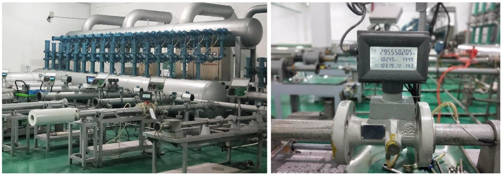
The sonic nozzle gas flow standard device (left) and swirl meter (right).
The experiment results are shown in Figure 17. The meter factor K was 34,756, 32,577, and 32,120 for the 11°, 20°, and 30° cone angles, respectively. Compared with prototype swirler (20°), the factor was about 6.7% higher when the cone angle decreased to 11° and about 1.4% lower when the cone angle increased to 30°. The simulation results are also shown in Figure 17. For a small flow condition (Q = 6 m3/h), the simulation error was relatively larger, while the error was less than 5% for the other flow conditions. Based on the results, the numerical method was adopted and the results show compelling evidence that our approach is reliable.
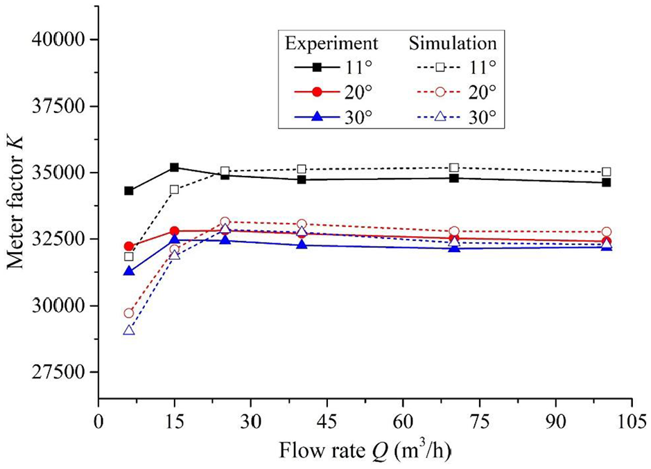
Experiment and simulation results of the meter factor K.
Conclusion
In this study, numerical simulations were conducted to investigate the internal characteristics of the swirl meter, and the results were verified by tests with the standard sonic nozzle gas flow device. The comparison of different flow conditions from 6 to 100 m3/h and the three swirler cone angles of 11°, 20°, and 30° were analyzed. The overall flow field distributions, pressure, and velocity profiles at the centerline and at different cross-sections were discussed in detail. Hence, our conclusions are as follows:
The mean pressure and velocity were the same at different flow conditions. Both of them were of centrosymmetric distribution and ensured that the swirl meter possesses a stable metering performance over a large range.
The flow acceleration was obvious in the convergent section; however, the pressure drop was also noticeable during this process. The overall pressure decreased gradually while it showed an opposite tendency on the centerline.
For the swirl meter with the 11° cone angle, a higher velocity was observed inside which results in a larger meter factor (6.8% larger than the 20° condition). The flow field distributions between the 20° and 30° cone angles were similar, such that the meter factor difference was only about 1.7%.
Swirler cone angle on internal flow of swirl meter was studied in this paper and proved to have direct influence on measurement characteristics. Therefore, an optimal design of the swirler and Venturi-like tube may conduct for future study to improve the measurement performance.
Footnotes
Declaration of conflicting interests
The author(s) declared no potential conflicts of interest with respect to the research, authorship, and/or publication of this article.
Funding
The author(s) disclosed receipt of the following financial support for the research, authorship, and/or publication of this article: This work was supported by the National Natural Science Foundation of China (Grant No. 51676174), the Key Research and Development Program of Zhejiang Province (Grant no. 2019C03117), the Public Projects of Zhejiang Province (Grant no. LGG19E060006), the Fundamental Research Funds of Zhejiang Sci-Tech University (Grant no. 2019Q037), and the Science Foundation of Zhejiang Sci-Tech University (Grant no. 18022222-Y).