Sage Journals: Discover world-class research

Abstract

Fluid, when running through pipes, makes a complex sound emission whose parameters change nonlinearly with respect to flow speed. Especially, in household pipe systems, there may be spraying effects and resonance effects which make the emission more complex. We present a novel approach for predicting flow speed based on wavelet packet analysis of sound emissions rather than traditional time and frequency domain methods. Wavelet packet analysis, by providing arbitrary time–frequency resolution, enables analyzing signals of stationary and non-stationary nature. It has better time representation than Fourier analysis and better high-frequency resolution than wavelet analysis. Wavelet packet analysis subimages are further analyzed to obtain feature vectors of norm entropy. These feature vectors are fed into a multilayer perceptron for prediction. Prediction accuracy of 98.62%, with 3.99E−04 L/s mean absolute error and its corresponding 1.85% relative error is achieved. Time sensitivity is ±0.453 s and is open to improvement by varying window width. The result indicates that the proposed method is a good candidate for flow measurement by acoustic analysis.

Keywords

Acoustic emissions flow measurement fluids multilayer perceptron norm entropy wavelet packet analysis

I. Introduction

Flow of a fluid can produce complex sound emissions in household pipe systems because of the spraying effects, resonances in the pipe structures and other mechanical interactions including friction. With highly varying parameters, this sound can hardly be used by linear methods to predict flow speed.

The possibility of pipe monitoring or flow measurement based on sound analysis has been investigated by researchers. Most of the researchers who worked on this subject have not reported measurement accuracies, but rough statistical correlations; for example, Dinardo et al.¹ and Campagna et al.² showed a linear dependence between the amplitude of the vibration acceleration in its frequency domain and the flow rate in a pipe and developed a fluid flow rate monitoring system; Campagna et al.² developed a methodology for the measurement of the fluid flow rate in a pipe, by means of appropriate evaluations to be implemented on the vibrational signals in the frequency domain; Dinardo et al.³ related the power content of the processed signals (by introducing the signal root mean square value) to the flow rate in a pipe; Saito et al.⁴ and Thompson et al.⁵ developed a relationship between pressure fluctuations caused by sudden flow rate changes; Evans et al.⁶ developed a flow rate measurement technique based on signal noise from an accelerometer attached to the surface of a pipe. They defined the signal noise as the standard deviation of the frequency averaged time-series signal and presented experimental results that indicate a nearly quadratic relationship between the signal noise and the mass flow rate in the pipe; Safari and Tavassoli⁷ showed empirical results that indicate that there is a relationship between the output signal of microphone in frequency domain and the flow rate in a pipe; Medeiros and Barbosa⁸ presented a method for measuring flow in pipelines based on the frequency domain values of vibration caused by the flow of water; and Hu et al.⁹ used accelerometer on a pipe to recognize the type of household water use activity.

Some of the researchers in this field reported measurement accuracies; for example, Jacobs et al.¹⁰ determined a mathematical relationship between the sound signal and the flow rate near a tap. Three models, based on Fourier transforms of data in the frequency domain, were devised to estimate the flow rate of water as a function of the audible sound signal properties. An average error of 15% was determined; Kim et al.¹¹ introduced a nonintrusive autonomous water monitoring system based on pipe dynamic theories to household plumbing in the form of an optimization problem and achieved flow measurement with 7% mean absolute error; and Kim et al.¹² used parameter estimation via numerical optimization technique to estimate flow rate with 5% average error.

Time domain, frequency domain (Fourier) and time–frequency domain (wavelet) analysis are the main tools used for analyzing signals but Fourier analysis has poor time representation and wavelet analysis has poor resolution at high frequency. Wavelet packet analysis (WPA), on the other hand, overcomes both of these, and the arbitrary time–frequency resolution enables analysis of signals of both stationary and non-stationary nature.

WPA has been successfully used to analyze signals for various applications; for example, Hu et al.¹³ used relative wavelet packet energy to classify surface electromyography (EMG) signals; Wang et al.¹⁴ used relative energy of harmonic wavelet packet to classify surface EMG signals; Wu and Liu¹⁵ used Shannon entropy of wavelet packet transform (WPT) for fault diagnosis in internal combustion engines; Ekici et al.¹⁶ used energy, norm entropy and Shannon entropy of WPT to locate fault on transmission lines; Hariharan et al.¹⁷ used energy and Shannon entropy of WPT for pathological infant cry analysis; Arjmandi and Pooyan¹⁸ used energy and Shannon entropy of WPT for pathological voice quality assessment; Yen and Lin¹⁹ used wavelet packet node energies to monitor vibration; Sekine et al.²⁰ used power of detail signals of wavelet packet decomposition (WPD) to classify waist acceleration signals; Averbuch et al.²¹ used energy of WPD to acoustically detect moving vehicles; Ting et al.²² used energy of WPD for electroencephalogram (EEG) feature extraction to be used in brain computer interfacing; Zhang et al.²³ used relative energy and Shannon entropy of WPD to automatically recognize cognitive fatigue from physiological indices; Crovato and Schuck²⁴ used Shannon entropy of WPD for classification of dysphonic voices; Subasi²⁵ used wavelet packet energy to classify EMG signals; Shao et al.²⁶ used wavelet packet energy to classify fault in gear; Zhang et al.²⁷ used wavelet packet energy for classification of power quality disturbance; Avci et al.²⁸ used norm entropy of WPD to recognize targets; Avci and Avci²⁹ used wavelet packet energy for digital radio signal classification; Toliyat et al.³⁰ used energy of WPD to detect railway defect; Alyt et al.³¹ used WPD and higher order statistics to detect and localize radio frequency (RF) radar pulses in noisy environment; Daqrouq³² used Shannon entropy of WPD for text-independent speaker identification; Avci³³ used norm, log energy and sure entropy of WPD to recognize a speaker; Behroozmand and Almasganj³⁴ used energy and Shannon entropy of WPD for classification of pathological speech; and Sengur et al.³⁵ used energy and norm entropy of WPD for texture classification.

In this work, we would like to predict the flow speed in a household water pipe system based on the analysis of emitted sound. For this purpose, we record sound under varying flow speed. We choose to make the analysis by WPA. Output of the WPA is a set of subsignals, number of which depends on the depth of the WPA. We choose norm entropy as a feature vector calculated from these subsignals. We look for a mapping tool from the feature vectors to the flow speed. Multilayer perceptron (MLP) provides such a possibility. It is a kind of neural network which is shown to be effective in black box modelling and function approximation.

II. Material

Sound emissions are recorded from 1.00 cm away from a household pipe with no contact to the pipe using a digital recorder attached to a microphone. Pipe has a circular cross section, made of steel and has a radius of 2.25 cm. The flow speed is varied in 11 even incremental steps between 0.0159 and 0.0526 L/s. Flow speed is measured using a volumetric method by keeping track of the time until fluid from the pipe fills a 1.0-L container. The flow speed is calculated by dividing 1.0 L by the time information from the chronometer. The digital recorder is set to a sampling rate of 44,100 Hz. Recordings from each flow speed are partitioned into 0.907-s long windows which provide us with a total of 110 windows for training and 110 for testing. The window width is selected as 40,000 time steps which we choose depending on our earlier experience in similar applications. Since each window is 0.907-s long, we have a time sensitivity of ±0.453 s. Figure 1 displays sample windows of signals from each of the 6 odd-numbered flow speeds out of 11 between 0.0159 and 0.0526 L/s.

Figure 1.

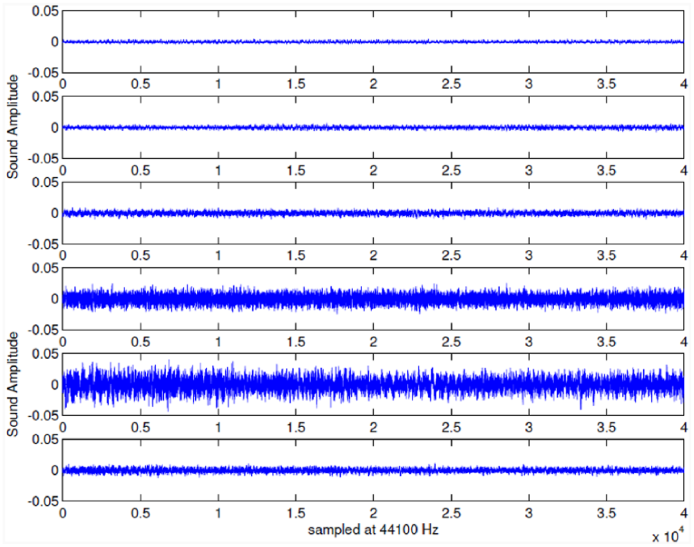
Sound signals recorded for odd-numbered 6 speeds out of 11 speeds (between 0.0159 and 0.0526 L/s) in increasing order from top to bottom

III. Method

Our analysis and prediction workflow is shown in Figure 2 . Each signal is first decomposed into wavelet packet subsignals by WPA. Then, features are extracted from these subsignals using norm entropy. These features are fed into our predictor, the MLP. By looking at prediction accuracy, we fine-tune the parameters: WPA depth, mother wavelet used and which nodes (all or final) of WPA to include in the prediction. Search is done by starting with the simplest parameters and increasing until the best prediction accuracy. The MLP parameters, which are the number of hidden layers and the number of neurons, are determined by pruning. This is to start with an MLP with one hidden layer with one neuron and increasing the number of layers and neurons until achieving the best accuracy. We analyze the contribution of each component of the feature vector corresponding to the nodes of WPA to prediction by a bar plot of the mean values of the feature vectors and then a box plot of the feature vectors at each of the WPD nodes at varying speeds. This lets us decide whether further reduction in the feature vector is needed.

Figure 2.

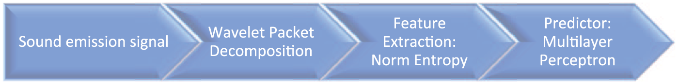
Classification workflow

A. WPD

WPD is used to decompose the signals. Wavelet packets are a generalization of wavelet bases by taking linear combinations of wavelet functions.³⁶ In the following explanation, we take a parallel approach to Yen and Lin¹⁹ and Wu and Liu.¹⁵

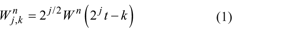
A wavelet function has three indices: j is the index scale (integer), k is the translation (integer), n is the oscillation parameter and t is the time

W_{j, k}^{n} = 2^{j / 2} W^{n} (2^{j} t - k)

(1)

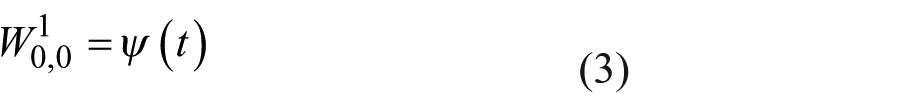
The first two wavelet packet functions are the scaling function and the mother wavelet function

W_{0, 0}^{0} = ϕ (t)

(2)

W_{0, 0}^{1} = ψ (t)

(3)

Wavelet packet functions with higher oscillation parameters are

W_{0, 0}^{2 n} = \sqrt{2} \sum_{k} h (k) W_{1, k}^{n} (2 t - k)

(4)

W_{0, 0}^{2 n + 1} = \sqrt{2} \sum_{k} g (k) W_{1, k}^{n} (2 t - k)

(5)

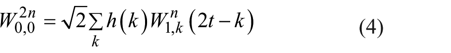
where h(k) and g(k) are quadrature mirror filters³⁷ associated with the scaling function and the mother wavelet function. The wavelet packet coefficients are defined as the inner product of wavelet packet functions with the input signal f(t), which also defines the range of t

w_{j, k}^{n} = f (t), W_{j, k}^{n} (t) = \int f (t) W_{j, k}^{n} (t) d t

(6)

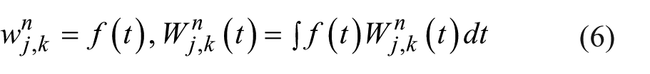
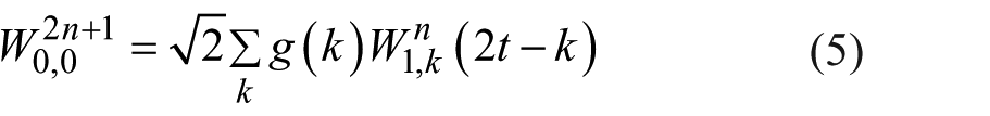
WPD is applied as shown in Figure 3 for three levels. The left-hand side sub-branches are obtained by low-pass filter h(k) and decimation; and the right-hand side sub-branches are obtained by high-pass filter g(k) and decimation. S is the original signal, A stands for approximation, D for detail and the number for level.

Figure 3.

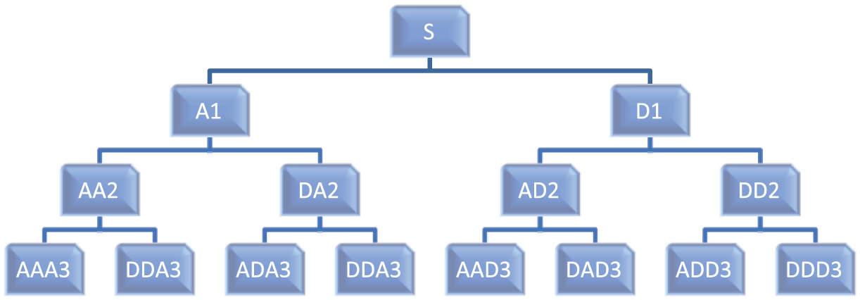
WPD tree up to three levels

B. Feature

Norm entropy is used as the feature vector for prediction. Entropy is a common measure used in signal processing which is able to extract useful information from a signal

Norm entropy : E = \sum_{n} {| w_{j, k}^{n} |}^{p}

(7)

where $w_{j, k}^{n}$ are the WPD coefficients calculated in equation (6) and 1 ≤ p.

C. Predictor: MLP

Various tools including neural networks are available for prediction. We choose MLP with backpropagation learning which can efficiently process large data sets and has been shown to be effective in black box modelling and function approximation.^38,39

MLP is a network of nodes arranged in layers. A node can be modeled as an artificial neuron that computes weighted sums of inputs with bias and presents it to an activation function. A general MLP model is shown in Figure 4 . Linear activation functions are used for input and output layers and hyperbolic tangent sigmoid activation functions for the hidden layer(s) which are in the following form

f (α) = \frac{2}{1 + e^{- 2 α}} - 1

(8)

Figure 4.

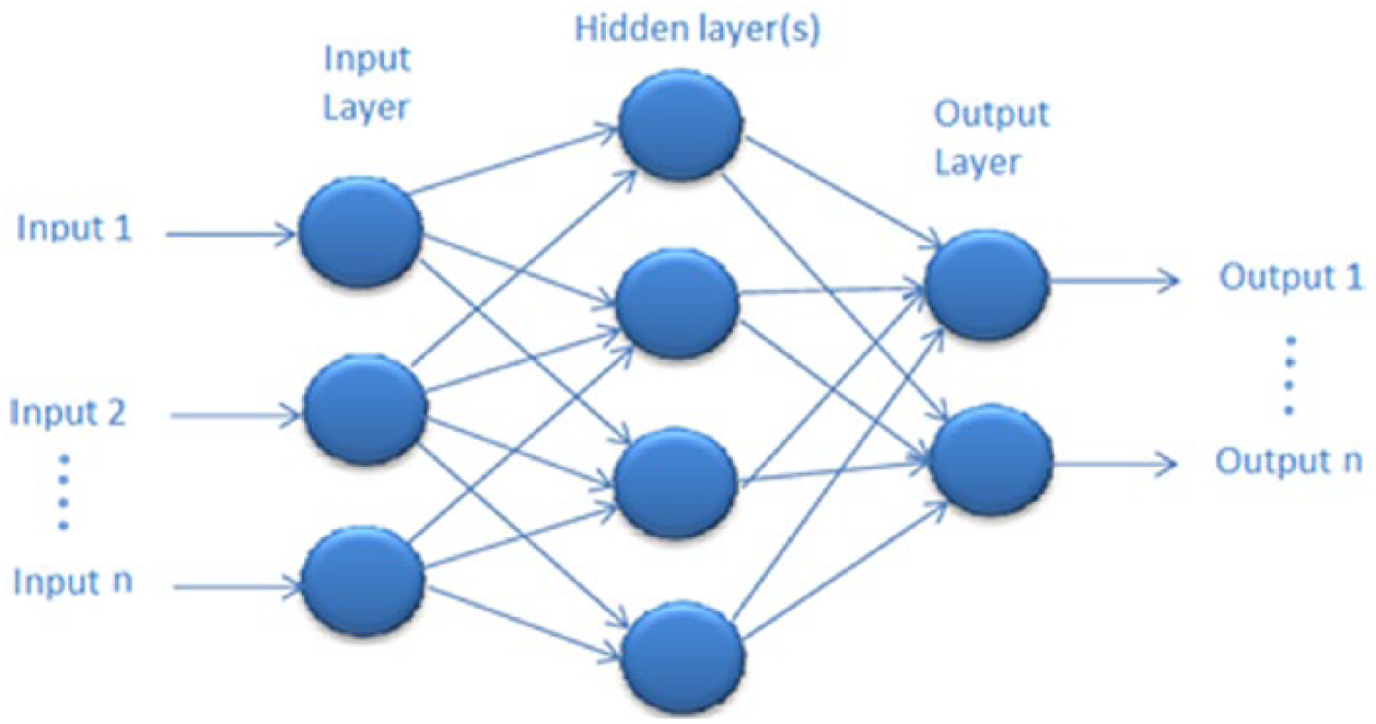
General architecture of the MLP

Training of the MLP is the adjustment of the weight parameters to map the input to the output with minimum error. For this purpose, backpropagation algorithm is adopted where the error between the actual output of the network and the target is backpropagated through the network to adjust the weight parameters.^40,41

IV. Results and Discussion

We start by WPD of the signals. We start at level 1 and increase the level until achieving the best prediction accuracy, which is at level 5. Final node of subsignals of WPD at depth 5 at speeds 0.0159 and 0.0526 L/s is shown in Figure 5 . Each vertical line is a subsignal. The WPD figures for two flow rates are visually different from each other at both the lower frequency (upper parts) and the higher frequency (lower parts) nodes in the WPD domain.

Figure 5.

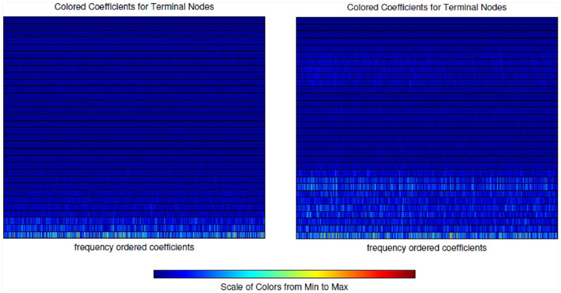
WPD of sound signals at speeds 0.0159 L/s (left) and 0.0526 L/s (right)

We calculate norm entropy of the final-level nodes of WPD. Bar plot of the mean values of the norm entropy for final 32 nodes of WPD for odd-numbered 6 speed steps out of 11 between flow rates 0.0159 and 0.0526 L/s is given in Figure 6 . This figure shows that feature vectors are different at various speeds and therefore will contribute to prediction.

Figure 6.

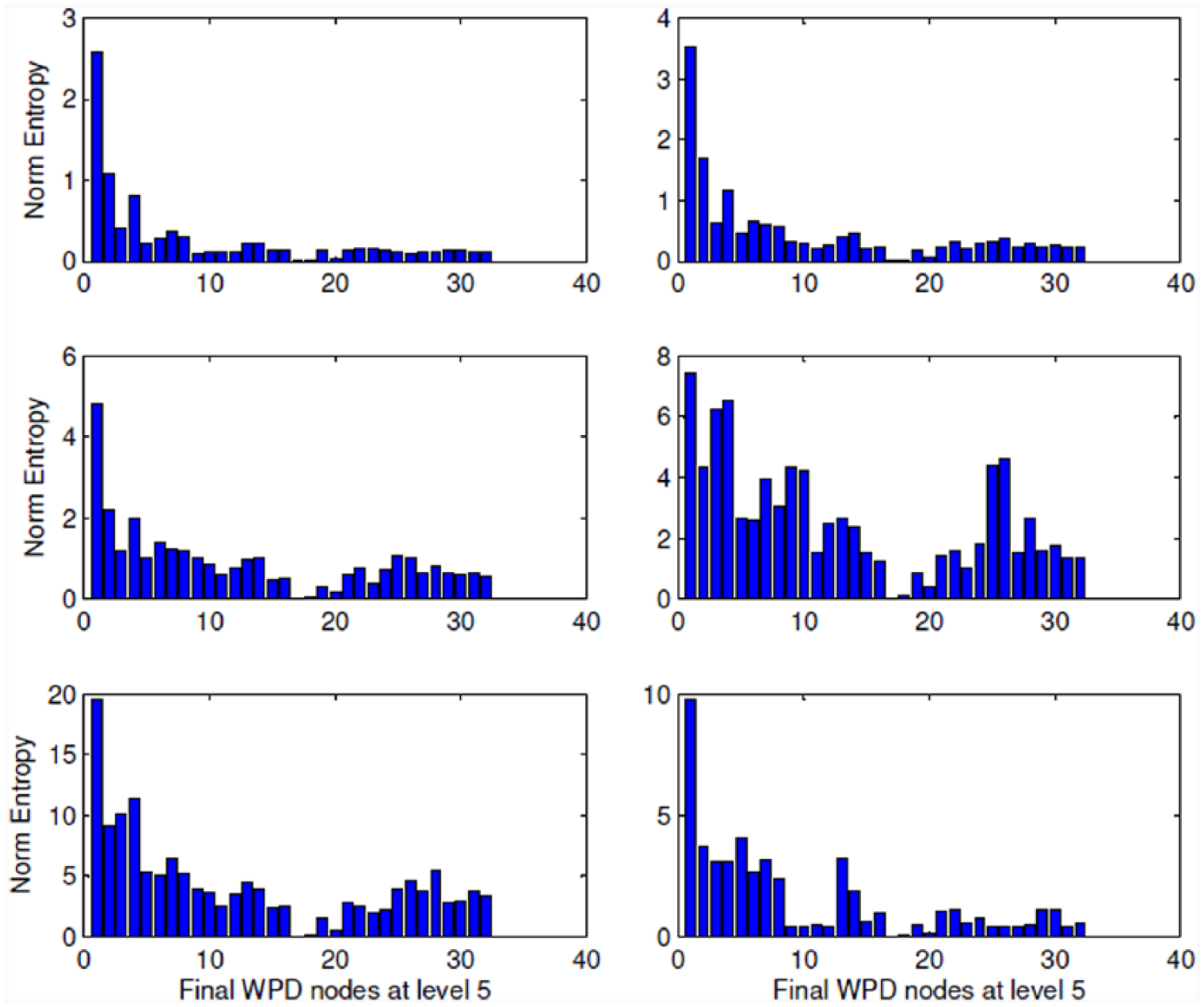
Mean values of norm entropy at final 32 nodes of WPD for odd-numbered 6 speed steps out of 11 between 0.0159 and 0.0526 L/s

To see how each WPD node is contributing to prediction more precisely, we box plot norm entropy for the same nodes of WPD corresponding to odd-numbered 6 speed steps out of 11 between 0.0159 and 0.0526 L/s in Figure 7 . In this figure, the central mark of each box is the median, the edges are the 25th and 75th percentiles and the whiskers cover the most extreme data points that are not outliers. Outliers are plotted individually as + signs. These plots show that feature vector at all nodes is different from each other at various flow rates so these will contribute to prediction; therefore, we decide not to make any reduction in the feature space.

Figure 7.

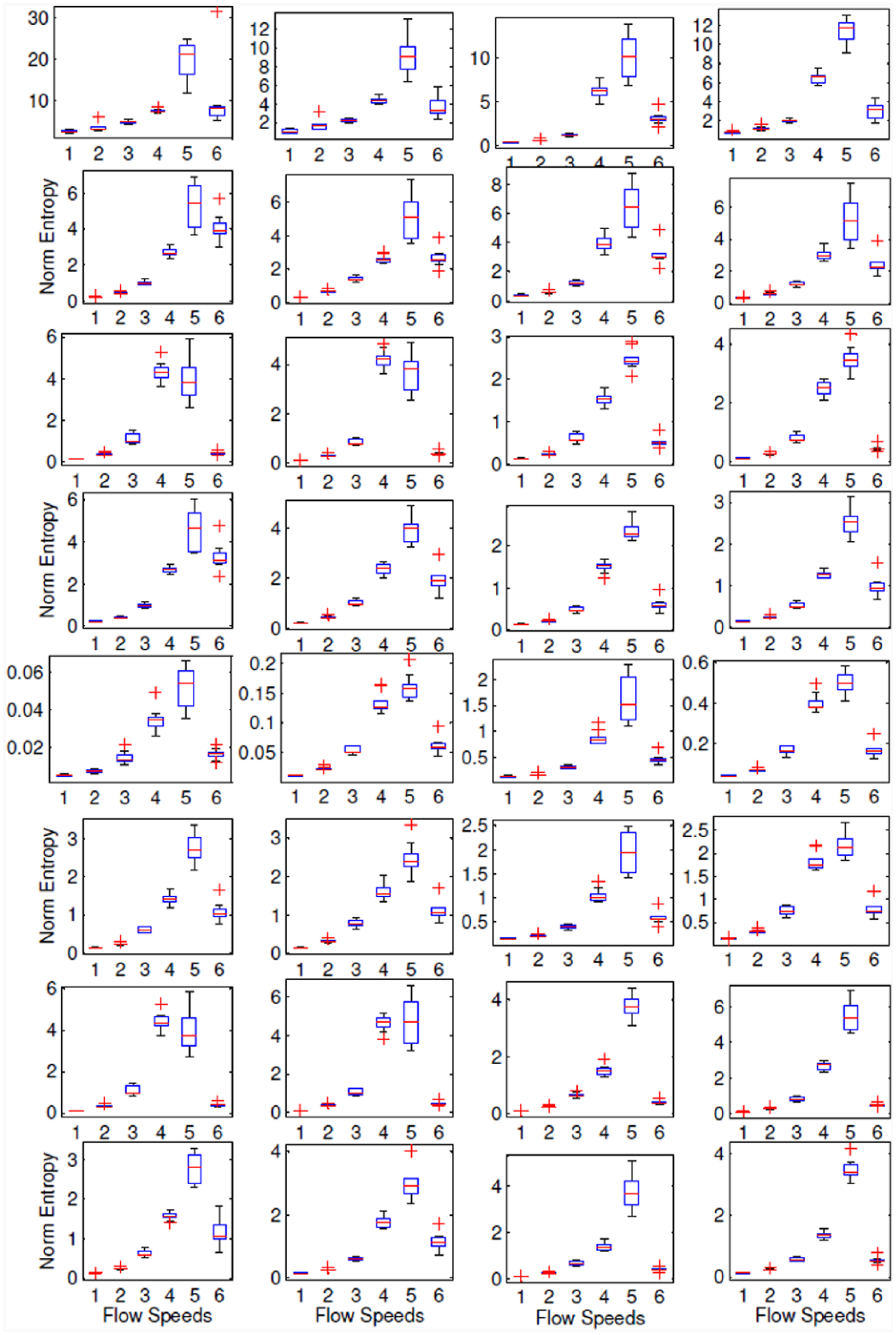
Box plot of norm entropy for 32 nodes of final level of WPD at depth 5 corresponding to odd-numbered 6 speed steps out of 11 between 0.0159 and 0.0526 L/s

We feed the norm entropy features into the MLP. We perform a search in the parameters: WPD depth, mother wavelet used, p value of norm entropy and WPD nodes used in prediction (all or final). We search by starting with the simplest or lowest value of the parameters and increase complexity until reaching the best prediction accuracy. Mother wavelet is found by a search in Daubechies wavelet family by starting with the simplest and increasing complexity until finding that db4 gives best prediction accuracy. Number of MLP hidden layers and the number of neurons are found by the method of pruning. This is to start with one hidden layer of one neuron and increase the number of layers and neurons until best prediction accuracy. The best parameter values that are found by the search, along with best average prediction accuracy, mean absolute prediction error and its corresponding relative error are given in Table 1 .

Table 1.

Parameters corresponding to best prediction accuracy

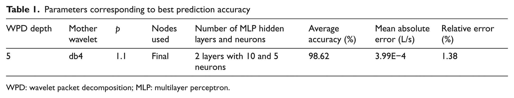
WPD depth	Mother wavelet	p	Nodes used	Number of MLP hidden layers and neurons	Average accuracy (%)	Mean absolute error (L/s)	Relative error (%)
5	db4	1.1	Final	2 layers with 10 and 5 neurons	98.62	3.99E−4	1.38

WPD: wavelet packet decomposition; MLP: multilayer perceptron.

Figure 8 shows the prediction result belonging to all test instances by plotting the actual and the predicted speeds. We see that prediction is mostly consistent with minor random fluctuations. Fluctuations can be linked to noise not related to flow which exists in some of the instances. We see that best prediction with 98.62% mean accuracy and 3.99E−4 L/s mean absolute error, which corresponds to 1.38% relative error, is accomplished with an MLP of two hidden layers with 10 and 5 neurons. Figure 9 shows the training performance of this best performing MLP.

Figure 8.

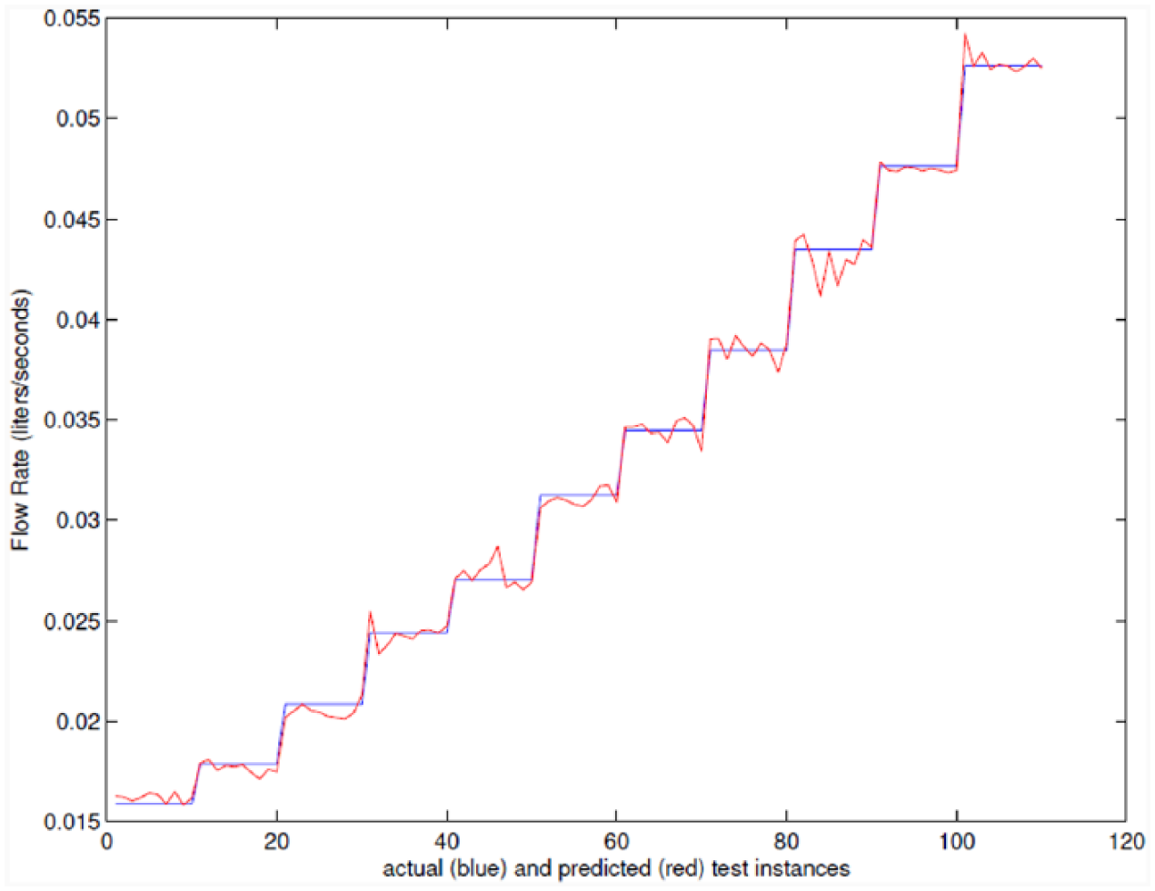
Actual speeds (blue) and predicted speeds (red) for all test instances corresponding to best prediction

Figure 9.

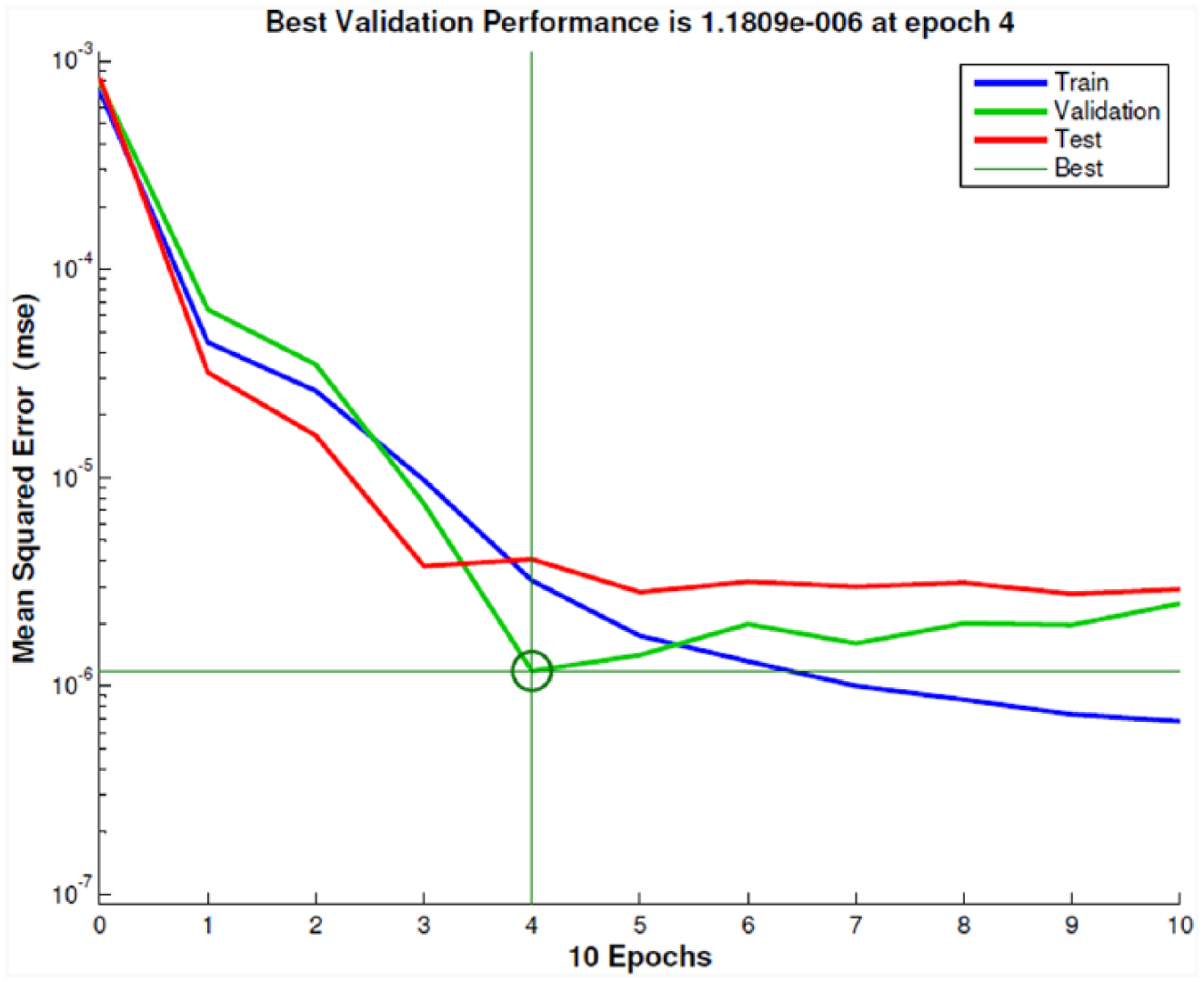
Training performance of the MLP with two hidden layers of 10 and 5 neurons

Most results that were reported in the literature review part of the “Introduction” section report rough statistical correlations in flow measurement by sound analysis. Three of them reported accuracy: Jacobs et al.¹⁰ who reported 85% accuracy using models based on Fourier transform; Kim et al.¹¹ who reported 93% accuracy using pipe dynamic theories parameter estimation; and Kim et al.¹² who reported 95% accuracy using parameter estimation via numerical optimization.

Although it is impossible to make a comparison between these results and ours, since all authors report results using different data sets, we can at least say that our result of flow measurement by WPA of sound emissions with 98.62% mean accuracy is among the good results. The result is in the household flow rate range of 0.0159–0.0526 L/s and further experimentation in other flow ranges is needed in order to generalize the method. The effect of the pipe material can also be investigated in a future research.

V. Conclusion

An approach for flow measurement by sound signal analysis is presented. WPA is chosen as the analysis tool and norm entropy is extracted as the feature vector from the wavelet packet subsignals. Prediction is done with an MLP. An average prediction accuracy of 98.62% with 3.99E−4 L/s mean absolute error and its corresponding 1.38% relative error is achieved. This result is in the household flow range of 0.0159–0.0526 L/s and is extendable to other ranges with further experimentation. Time sensitivity is ±0.453 s and is open to improvement by exploring different window widths. Experimentation with other pipe materials can be done in a future research. The method according to the given results presents us with a promising tool for flow speed measurement by sound emission analysis. It opens the way for a new kind of lower cost, portable and noninvasive flow sensor which can be used to monitor flow in pipe systems.

Footnotes

Funding

The author(s) received no financial support for the research, authorship and/or publication of this article.

Conflict of interest

The author(s) declared no potential conflicts of interest with respect to the research, authorship and/or publication of this article.

ORCID iD

Hüseyin Göksu

References

Dinardo

Fabbiano

Vacca

Fluid flow rate estimation using acceleration sensors. In Proceedings of the 2013 seventh international conference on sensing technology (ICST), Wellington, New Zealand, 3–5 December 2013, pp.221–5. New York: IEEE.

Campagna

Dinardo

Fabbiano

Vacca

Fluid flow measurements by means of vibration monitoring. Measurement Science and Technology 2015; 26(11): 115306.

Dinardo

Fabbiano

Vacca

Lay-Ekuakille

Vibrational signal processing for characterization of fluid flows in pipes. Measurement 2018; 113: 196–204.

Saito

Miyano

Furukawa

Study on vibration response of pipes induced by internal flow. In Pressure vessels and piping conference, Nashville, TN, 17-21 June 1990, pp.233–8. New York: ASME.

Thompson

Maynes

Blotter

JD.

Internal turbulent flow induced pipe vibrations with and without baffle plates. In ASME 2010 3rd Joint US-European fluids engineering summer meeting collocated with 8th international conference on nanochannels, microchannels, and minichannels, Montreal, QC, Canada, 1–5 August 2010, pp.649–59. New York: ASME.

Evans

Blotter

Stephens

AG.

Flow rate measurements using flow-induced pipe vibration. Journal of Fluids Engineering 2004; 126(2): 280–5.

Safari

Tavassoli

Initial test and design of a soft sensor for flow estimation using vibration measurements. In Proceedings of the 2nd international conference on control, instrumentation and automation (ICCIA), Shiraz, Iran, 27–29 December 2011, pp.809–14. New York: IEEE.

Medeiros

Barbosa

CR.

Nonintrusive method for measuring water flow in pipes. In XXI IMEKO world congress “measurement in research and industry,” Prague, Czech Republic, 30 August–4 September 2015.

Chen

Wang

Jia

A nonintrusive and single-point infrastructure-mediated sensing approach for water-use activity recognition. In Proceedings of the IEEE 10th international conference on high performance computing and communications and 2013 IEEE international conference on embedded and ubiquitous computing (HPCC_EUC), Zhangjiajie, China, 13–15 November 2013, pp.2120–6. New York: IEEE.

10.

Jacobs

Skibbe

Makwiza

Correlating sound and flow rate at a tap. Procedia Engineering 2015; 119: 864–73.

11.

Kim

Schmid

Charbiwala

Friedman

Srivastava

MB.

NAWMS: Nonintrusive autonomous water monitoring system. In Proceedings of the 6th ACM conference on embedded network sensor systems, Raleigh, NC, 5–7 November 2008, pp.309–22. New York: ACM.

12.

Kim

Park

Srivastava

MB.

A longitudinal study of vibration-based water flow sensing. ACM T Sensor Network 2012; 9(1): 8.

13.

Wang

Ren

Classification of surface EMG signal using relative wavelet packet energy. Computer Methods and Programs in Biomedicine 2005; 79(3): 189–95.

14.

Wang

Yan

Xie

Wang

Classification of surface EMG signals using harmonic wavelet packet transform. Physiological Measurement 2006; 27(12): 1255–67.

15.

Liu

CH.

An expert system for fault diagnosis in internal combustion engines using wavelet packet transform and neural network. Expert Systems with Applications 2009; 36(3): 4278–86.

16.

Ekici

Yildirim

Poyraz

Energy and entropy-based feature extraction for locating fault on transmission lines by using neural network and wavelet packet decomposition. Expert Systems with Applications 2008; 34(4): 2937–44.

17.

Hariharan

Yaacob

Awang

SA.

Pathological infant cry analysis using wavelet packet transform and probabilistic neural network. Expert Systems with Applications 2011; 38(12): 15377–82.

18.

Arjmandi

Pooyan

An optimum algorithm in pathological voice quality assessment using wavelet-packet-based features, linear discriminant analysis and support vector machine. Biomedical Signal Processing and Control 2012; 7(1): 3–19.

19.

Yen

Lin

KC.

Wavelet packet feature extraction for vibration monitoring. IEEE Transactions on Industrial Electronics 2000; 47(3): 650–67.

20.

Sekine

Tamura

Togawa

Fukui

Classification of waist-acceleration signals in a continuous walking record. Medical Engineering and Physics 2000; 22(4): 285–91.

21.

Averbuch

Zheludev

Rabin

Schclar

Wavelet-based acoustic detection of moving vehicles. Multidimensional Systems and Signal Processing 2009; 20(1): 55–80.

22.

Ting

Guo-Zheng

Bang-Hua

Hong

EEG feature extraction based on wavelet packet decomposition for brain computer interface. Measurement 2008; 41(6): 618–25.

23.

Zhang

Zheng

XL.

Automatic recognition of cognitive fatigue from physiological indices by using wavelet packet transform and kernel learning algorithms. Expert Systems with Applications 2009; 36(3): 4664–71.

24.

Crovato

CDP

Schuck

The use of wavelet packet transform and artificial neural networks in analysis and classification of dysphonic voices. IEEE Transactions on Biomedical Engineering 2007; 54(10): 1898–900.

25.

Subasi

Classification of EMG signals using combined features and soft computing techniques. Applied Soft Computing 2012; 12(8): 2188–98.

26.

Shao

Wang

The fault feature extraction and classification of gear using principal component analysis and kernel principal component analysis based on the wavelet packet transform. Measurement 2014; 54: 118–32.

27.

Zhang

Classification of power quality disturbances using wavelet packet energy and multiclass support vector machine. COMPEL: The International Journal for Computation and Mathematics in Electrical and Electronic Engineering 2012; 31(2): 424–42.

28.

Avci

Turkoglu

Poyraz

Intelligent target recognition based on wavelet packet neural network. Expert Systems with Applications 2005; 29(1): 175–82.

29.

Avci

A novel approach for digital radio signal classification: Wavelet packet energy–multiclass support vector machine (WPE–MSVM). Expert Systems with Applications 2008; 34(3): 2140–7.

30.

Toliyat

Abbaszadeh

Rahimian

Olson

LE.

Rail defect diagnosis using wavelet packet decomposition. IEEE Transactions on Industry Applications 2003; 39(5): 1454–61.

31.

Alyt

Omar

Elsherbeni

AZ.

Detection and localization of RF radar pulses in noise environments using wavelet packet transform and higher order statistics. Progress in Electromagnetics Research 2006; 58: 301–17.

32.

Daqrouq

Wavelet entropy and neural network for text-independent speaker identification. Engineering Applications of Artificial Intelligence 2011; 24(5): 796–802.

33.

Avci

A new optimum feature extraction and classification method for speaker recognition: GWPNN. Expert Systems with Applications 2007; 32(2): 485–98.

34.

Behroozmand

Almasganj

Optimal selection of wavelet-packet-based features using genetic algorithm in pathological assessment of patients’ speech signal with unilateral vocal fold paralysis. Computers in Biology and Medicine 2007; 37(4): 474–85.

35.

Sengur

Turkoglu

Ince

MC.

Wavelet packet neural networks for texture classification. Expert Systems with Applications 2007; 32(2): 527–33.

36.

Wickerhauser

MV.

Adapted Wavelet Analysis from Theory to Software. AK Peters, Wellesley, MA, 1994.

37.

Akansu

Haddad

RA.

Multiresolution Signal Decomposition: Transforms, Subbands, and Wavelets. Academic Press, Cambridge, MA, 2001.

38.

Lippmann

RP.

Pattern classification using neural networks. IEEE Communications Magazine 1989; 27(11): 47–50.

39.

Roth

MW.

Survey of neural network technology for automatic target recognition. IEEE Transactions on Neural Networks 1990; 1(1): 28–43.

40.

Rumelhart

Durbin

Golden

Chauvin

. Backpropagation: Theory, Architectures, and Applications. L. Erlbaum Associates Inc., Nahwah, NJ, 1995.

41.

Wang

McFadden

PD.

Application of orthogonal wavelets to early gear damage detection. Mechanical Systems and Signal Processing 1995; 9(5): 497–507.

Flow Measurement by Wavelet Packet Analysis of Sound Emissions

Abstract

Keywords

I. Introduction

II. Material

III. Method

A. WPD

B. Feature

C. Predictor: MLP

IV. Results and Discussion

V. Conclusion

Footnotes

Funding

Conflict of interest

ORCID iD

References