Sage Journals: Discover world-class research

Abstract

A vehicle, when running, makes a complex sound emission from the engine, the exhaust, the air conditioner, and other mechanical parts. Analysis of this sound for the purpose of vehicle identification is an interesting practice which has security- and transportation-related applications. Engine speed variation, which causes shifts in the frequency content of the emissions, makes Fourier-based methods ineffective in terms of providing a stable signature for the vehicle. We search for an engine speed–independent acoustic signature for the vehicle, and for this purpose, we propose wavelet packet analysis rather than traditional time- or frequency-domain methods. Wavelet packet analysis, by providing arbitrary time–frequency resolution, enables analyzing signals of stationary and non-stationary nature. It has better time representation than Fourier analysis and better high-frequency resolution than wavelet analysis. Under varying engine speed, sound emissions are recorded from four cars and analyzed by wavelet packet analysis. Wavelet packet analysis subimages are further analyzed to obtain feature vectors in the form of log energy entropy, norm entropy, and energy. These feature vectors are fed into a classifier, multilayer perceptron, for evaluation. While norm entropy achieves a classification rate of 100%, log energy entropy and energy achieves classification rates of 99.26% and 97.79%, respectively. These results indicate that, wavelet packet analysis along with norm entropy and multilayer perceptron provides an accurate vehicle-specific acoustic signature independent of the engine speed.

Keywords

Acoustic analysis MLP norm entropy vehicle identification wavelet packet analysis

I. Introduction

A vehicle, when running, produces a complex sound emission from its engine, the exhaust, air conditioner, and other mechanical parts and, if it is moving, from tires and air friction. With highly varying parameters, this sound carries certain diagnostic values including vehicle detection and identification and information regarding fault diagnosis. The possibility of identification and diagnosis of vehicles based on the analysis of sound emissions has been investigated by researchers. Various methods have been proposed to analyze the signals. Below is a chronological review of time-domain, frequency-domain, time–frequency domain, and hybrid analysis methods used in vehicle acoustic signal analysis.

Some of the researchers used time-domain features, for example, Mazarakis and Avaritsiotis¹ used a time-domain encoding and feature extraction to classify tracked vehicles and heavy trucks using their acoustic and seismic signatures; Paulraj et al.² used multi-frame time-domain features for classification of moving vehicles; Wang and Zhou³ used improved time-encoded signal-processing algorithm for feature extraction in acoustic vehicle-type recognition; Rahim et al.⁴ used time-domain features for the classification of moving vehicles; Paulraj et al.⁵ used autoregressive modeling for vehicle-type classification; Mayvan et al.⁶ used quadratic discriminant analysis to classify audio signals of passing vehicles to bus, car, motor, and truck categories based on features such as short-time energy, average zero-crossing rate, and pitch frequency of periodic segments of signals; and Ishida et al.⁷ used dynamic time warping to design an acoustic vehicle-count system.

Some of the researchers used frequency-domain features, for example, Nooralahiyan et al.⁸ used linear predictive coding coefficients, auditory model processing and Fourier transform for acoustic signature analysis for vehicle classification; Wu et al.⁹ used frequency vector principal component analysis for vehicle sound signature recognition; Nooralahiyan et al.¹⁰ used linear predictive coding for vehicle classification by acoustic signature; Munich¹¹ used a probabilistic classifier that is trained on the principal components subspace of the short-time Fourier transform for acoustic signature recognition of vehicles; Sun and Daigle¹² used fast Fourier transform (FFT) magnitudes for vehicle classification; Yang et al.¹³ used overall shape of sound spectrum for vehicle identification; Malhotra et al.¹⁴ used features based on FFT and power spectral density (PSD) to classify running vehicles; Yang et al.¹⁵ used discrete spectrums to identify vehicles in wireless sensor networks; Lu et al.¹⁶ used spectral features to classify running vehicle types into gasoline light-wheeled, gasoline heavy-wheeled, diesel truck and motorcycle; Lu et al.¹⁷ used gammatone filterbanks as spectral features for detecting acoustic signature of approaching vehicles; Malhotra et al.¹⁸ used PSD-based features for classifications in audio-sensor networks; Guo et al.¹⁹ used a number of harmonic components and a group of key frequency components for ground vehicle classification; Bikdash et al.²⁰ used tristimulus response for classification of civilian vehicles from acoustic data; Malhotra et al.²¹ used Aura matrices to create a new feature derived from the PSD and dynamic multidimensional PSD for vehicle classification by wireless audio-sensor networks; Kozhisseri and Bikdash²² used spectral features for the classification of civilian vehicles using acoustic sensors; Changjun and Yuzong²³ used short-time Fourier transform of acoustic and seismic signals for vehicle classification; Rahim et al.²⁴ used one-third octave filter bands for moving vehicle noise classification; Özgündüz et al.²⁵ used Mel-frequency cepstral coefficients for vehicle identification using acoustic and seismic signals; Mato-Mendez and Sobreira-Seoane²⁶ used Mel-frequency cepstral coefficients, sub-band energy ratio, spectral centroid, and spectral roll-off point to classify vehicles; Zhao et al.²⁷ used PSD to recognize status of ball mill load using shell vibration signal; Bhave and Rao²⁸ used formant-based feature and Mel-frequency cepstral coefficients for vehicle engine sound analysis applied to traffic congestion estimation; Gorski and Zarzycki²⁹ used Harmonic line, Shur coefficients and Mel filters methods for feature extraction in acoustic vehicle classification; Guo et al.³⁰ used a number of harmonic components and a group of key frequency components for ground vehicle classification; Rahim et al.³¹ used one-third octave filter band for moving vehicle classification; Rahim et al.³¹ used one-third octave frequency spectrum analysis to classify type and the distance of a moving vehicle with types: car, bike, lorry, and truck; Biernacki³² used harmonic features and correlation features for acoustic vehicle identification; Zambon et al.³³ used a database of vehicles to statistically analyze one-third octave band spectra of emission noise in terms of its relevance to vehicle speed; Sunu and Percus³⁴ used frequency signatures to classify vehicles; and Zambon et al.³⁵ used statistical analysis of recorded spectra of vehicles to detect its relevance to vehicle speed.

Some of the researchers used time–frequency domain features, for example, Averbuch et al.³⁶ used wavelet packet energy for the classification and detection of moving vehicles; Lu et al.³⁷ assembled gammatone feature vectors over multiple temporal frames to establish a high dimensional spectro-temporal representation for noise-independent vehicle sound recognition; Averbuch et al.³⁸ used energy of wavelet packet transform (WPT) for acoustic detection of moving vehicles; and Schclar et al.³⁹ used total magnitude (L1 norm) of the coefficients from wavelet packet decomposition (WPD) to detect vehicles.

Some of the researchers used hybrid features, for example, Aljaafreh and Dong⁴⁰ used PSD of short-time Fourier spectrum and energy of WPT for vehicle classification based on acoustic signals; Padmavathi et al.⁴¹ used signal energy, energy entropy, zero-crossing rate, spectral roll-off, spectral centroid, and spectral flux for vehicle acoustic signal classification; Aljaafreh and Al-Fuqaha⁴² used spectrum analysis and energy of WPT for acoustic classification of multiple targets; George et al.⁴³ used short-time energy, log energy, and smoothed log energy for vehicle detection and Mel-frequency cepstral coefficients for vehicle classification; Kakar and Kandpal⁴⁴ reviewed time-domain, frequency-domain and time–frequency domain feature extraction methods that are used in classification of vehicles; and Shah and Mehta⁴⁵ used time-domain and frequency-domain features for the analysis of acoustic signals for vehicle classification of four wheeler models.

Time-domain, frequency-domain (Fourier), and time–frequency domain (Wavelet) analysis are the main tools for analyzing signals, but Fourier analysis has poor time representation and wavelet analysis has poor resolution at high frequency. Wavelet packet analysis (WPA) overcomes both of these, and the arbitrary time–frequency resolution enables analysis of signals of both stationary and non-stationary nature.

In search for an engine speed–independent acoustic signature for vehicles, we propose a method based on WPA of the sound signals for the aforementioned reasons. Moreover, since frequency content of the signals shifts under varying engine speeds, Fourier-based methods would not provide a stable signature. To apply the proposed method, we record sound emissions from four vehicles by varying the engine speed. Output of the WPA is a set of subsignals. We analyze these subsignals further using norm entropy, log energy entropy, and energy. For classification, we feed these feature vectors to a multilayer perceptron, which is a kind of neural network that is able to learn patterns from a set of data and generalize to a new set. It has been shown to be effective in pattern recognition and classification problems. We evaluate the three features given for their classification accuracy.

II. Material

Sound emissions are recorded from four vehicles: a Ford Kuga 1.5 L Ecoboost, a Skoda Fabia 1.4 L, a Volkswagen Passat 1.6 L TDi, and a Ford Tourneo Courier 1.5 L TDCi. Measurements are made using a digital recorder attached to a microphone with a sampling rate of 44,100 Hz. Recordings are taken from a location 1 m away from the engine on the left side of the vehicle. We choose this as a reasonable distance to be used in a real vehicle detection and identification system. Since the minimum idle running speed of the vehicle engines is 800 r/min, we start at that rate and increase until 3000 r/min. An RPM ranging around 800–3000 r/min is chosen because it is the usual running range of the vehicle engines unless aggressive driving. We increase the engine speed slowly beginning with 800 r/min going up to 3000 r/min and then decrease back, which we repeat two times. We would like about 30 training samples and 30 test samples from each vehicle, each of which is 0.907 s long in order to contain 40,000 time steps. We choose this window width based on our earlier experience in similar problems. In order to obtain aforementioned training and test samples, we arrange each increase and decrease episode to be roughly 30 s. Figure 1 shows 1 min recordings from each vehicle which include two episodes of increase and decrease of engine speeds. The first increase and decrease episodes are used to extract training samples, and the second episodes are used to extract test samples. This procedure ensures that training and test samples contain sound emissions from the whole range of engine speeds between 800 and 3000 r/min. Total number of training samples is 130 and testing samples is 136.

Figure 1.

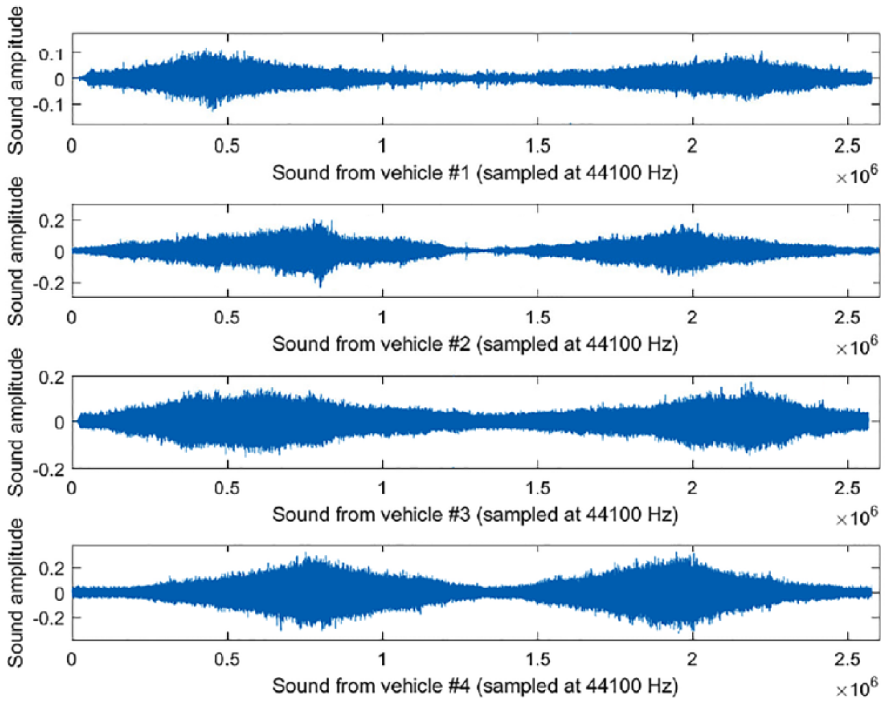
Sound signals recorded from four vehicles.

III. Method

Our analysis and classification workflow is such that each signal is first decomposed into wavelet packet subsignals by WPA. Then features are extracted from these subsignals in the form of norm entropy, log energy entropy, and energy. To evaluate these features we feed them into a classifier, multilayer perceptron (MLP). During this procedure, we fine tune the following parameters: WPA depth, mother wavelet used, which nodes (all or final) of WPA to include in the analysis, and the neural network parameters.

We analyze the contribution of each component of the feature vector which corresponds to the nodes of WPA by a barplot of the mean values and then a boxplot of the feature at each node of the WPA for each vehicle. These let us to decide whether a reduction in the feature vectors or further fine-tuning of parameters is needed.

A. WPD

WPD is used to decompose the signals. Wavelet packets are a generalization of wavelet bases by taking linear combinations of wavelet functions.⁴⁶ In the following explanation, we take a parallel approach to Yen and Lin⁴⁷ and Wu and Liu.⁴⁸

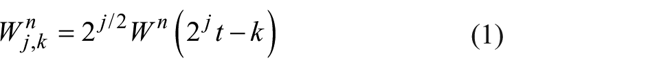
A wavelet function has three indices, j: index scale (integer), k: translation (integer), n: oscillation parameter; and t is time

W_{j, k}^{n} = 2^{j / 2} W^{n} (2^{j} t - k)

(1)

The first two wavelet packet functions are a scaling function and the mother wavelet function

W_{0, 0}^{0} = ϕ (t)

(2)

W_{0, 0}^{1} = ψ (t)

(3)

Wavelet packet functions with higher oscillation parameters are

W_{0, 0}^{2 n} = \sqrt{2} \sum_{k} h (k) W_{1, k}^{n} (2 t - k)

(4)

W_{0, 0}^{2 n + 1} = \sqrt{2} \sum_{k} g (k) W_{1, k}^{n} (2 t - k)

(5)

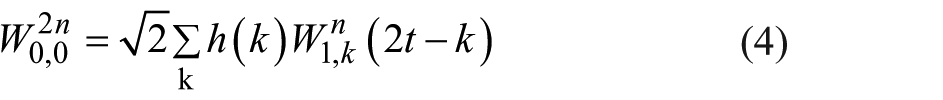
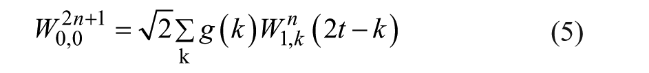
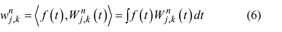
where h(k) and g(k) are quadrature mirror filters⁴⁹ associated with the scaling function and the mother wavelet function. The wavelet packet coefficients are defined as the inner product of wavelet packet functions with the input signal f(t), which also defines the range of t

w_{j, k}^{n} = 〈 f (t), W_{j, k}^{n} (t) 〉 = \int^{} f (t) W_{j, k}^{n} (t) d t

(6)

WPD is applied as shown in Figure 2 for three levels. The left hand–side sub-branches are obtained by low-pass filter h(k) and decimation; the right hand–side sub-branches are obtained by high-pass filter g(k) and decimation. S is the original signal, A stands for approximation, D for detail, and the number for level.

Figure 2.

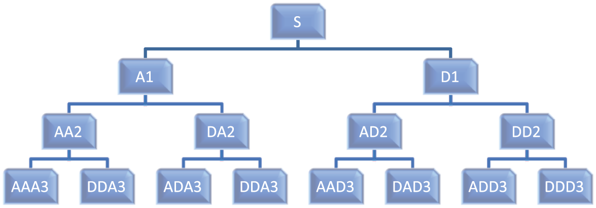
WPD tree up to three levels.

B. Feature

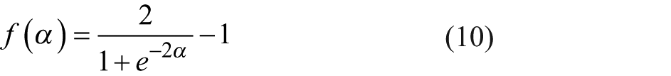
Norm entropy, log energy entropy, and energy are used as feature vectors for prediction. Entropy and energy are common measures used in signal processing, which are able to extract useful information from a signal

Norm entropy : E = {\sum_{n} | w_{j, k}^{n} |}^{p}

(7)

Log energy entropy : E = \sum_{n} l o g (w_{j, k}^{n 2})

(8)

Energy : E = \sum_{n} w_{j, k}^{n 2}

(9)

where $w_{j, k}^{n}$ are the WPD coefficients calculated in equation (6) and 1 ≤ p.

C. Classifier: MLP

Various tools including neural networks are available for classification. We choose MLP with backpropagation learning which can efficiently process large data sets and has been shown to be effective in pattern recognition and classification.^50,51

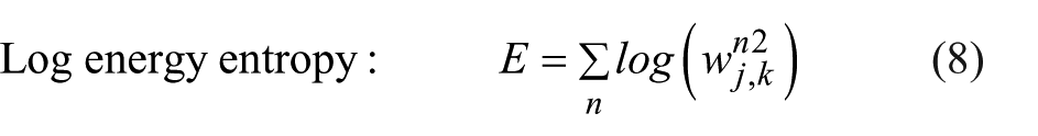
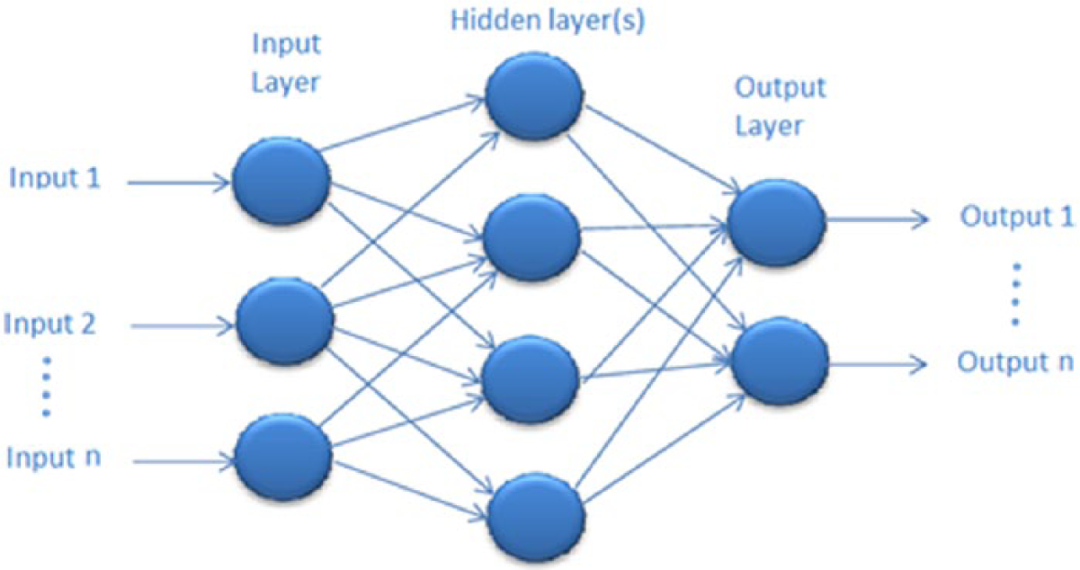
MLP is a network of nodes arranged in layers. A node can be modeled as an artificial neuron that computes weighted sums of inputs with bias and presents it to an activation function. A general MLP model is shown in Figure 3 . Linear activation functions were used for input and output layers and hyperbolic tangent sigmoid activation function for the hidden layer(s) which are in the form

f (α) = \frac{2}{1 + e^{- 2 α}} - 1

(10)

where a is the input to the neuron. Training of the MLP is the adjustment of the weight parameters to map the input to the output with minimum error. For this purpose, backpropagation algorithm is adopted where the error between the actual output of the network and the target is backpropagated through the network to adjust the weight parameters.^52,53

Figure 3.

General architecture of the MLP.

IV. Results and Discussion

We start by WPD of the signals at level 1 and increase until level 5, which gives the best classification accuracy. We search the Daubechies mother wavelet space by starting with the simplest and increasing complexity until reaching best accuracy at db4. First, we include all nodes of WPD up to the final level and then switch to using only the final nodes which gives better accuracy. Figure 4 shows the WPD of signals at 800, 2000, and 3000 r/min for each vehicle. Each horizontal line represents a subimage, and low-frequency nodes are in the upper region. Visually, vehicles 3 and 4 are easily differentiable from each other and from vehicles 1 and 2. MLP parameters, the number of hidden layers, and the number of neurons are determined by the method of pruning. This is to start with one hidden layer of 1 neuron and increase until reaching the best classification accuracy at two layers with eight and four neurons. p-value of the norm entropy is again defined by a search in the interval (1, 2) with 0.1 increments. Best-performing parameters are given in Table 1 , along with the classification accuracy achieved by each of the three features: norm entropy, log energy entropy, and energy.

Figure 4.

WPD of signals at speeds 800, 2000, and 3000 r/min.

Table 1.

Best-performing parameter values and accuracies achieved.

WPD depth	Mother wavelet	Feature	p	Nodes	MLP hidden layers	Classification accuracy (%)
5	db4	Energy	–	Final	2 layers, 8 and 4 neurons	97.79
5	db4	Log energy entropy	–	Final	2 layers, 8 and 4 neurons	99.26
5	db4	Norm entropy	1.1	Final	2 layers, 8 and 4 neurons	100

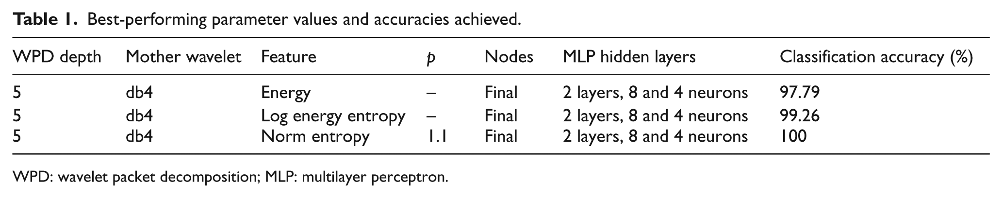
WPD: wavelet packet decomposition; MLP: multilayer perceptron.

Norm entropy achieves 100% classification accuracy with p = 1.1, and energy and log energy entropy achieves accuracies of 97.79% and 99.26%, respectively.

We plot mean values of norm entropy corresponding to final 32 nodes of WPD for each vehicle in Figure 5 . It is easy to see that mean of the feature vector is very different for each vehicle. In order to see the contribution of each node of WPD, we boxplot norm entropy of four vehicles at each node of the WPD in Figure 6 . The central mark of each box is the median, the edges are the 25th and 75th percentiles, and the whiskers cover the most extreme data points that are not outliers. Outliers are plotted individually. In these plots, it is easy to see that norm entropy ranges for each vehicle is mostly different from the others in most of the nodes. But it is hard to estimate the contribution of each node, so we keep all of the nodes in the analysis and decide not to make any reduction in the feature space. Reduction, which might reduce the complexity of the method, can be considered as a future work, but it is not essential since we have reached 100% classification accuracy, so we have found the right feature which provides a precise engine speed–independent acoustic signature for vehicles: WPA followed by norm entropy and MLP. Figure 7 shows the training performance of the best-performing MLP for the classification when feature is norm entropy.

Figure 5.

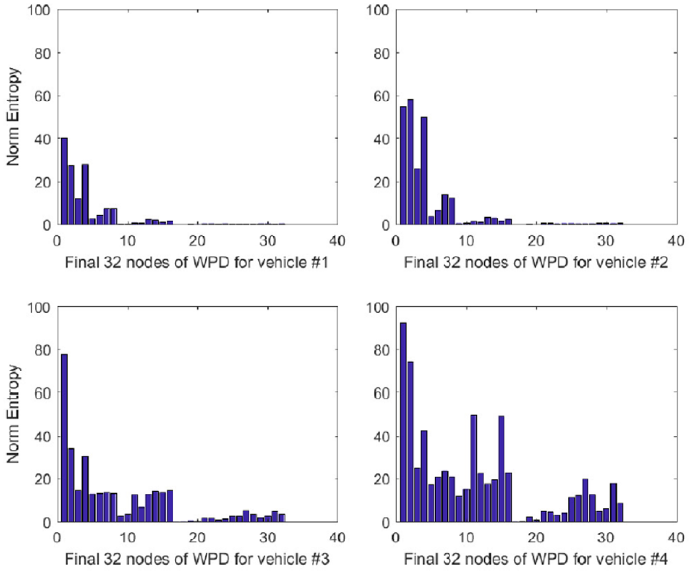
Mean values of norm entropy for final 32 nodes of WPD for four vehicles.

Figure 6.

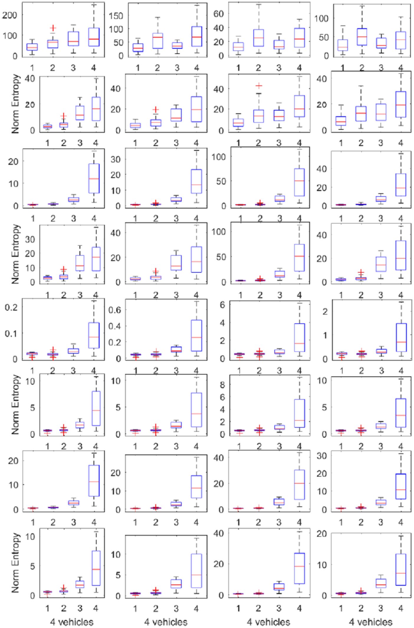
Boxplot of norm entropy at final 32 nodes of WPD at depth 5 for four vehicles.

Figure 7.

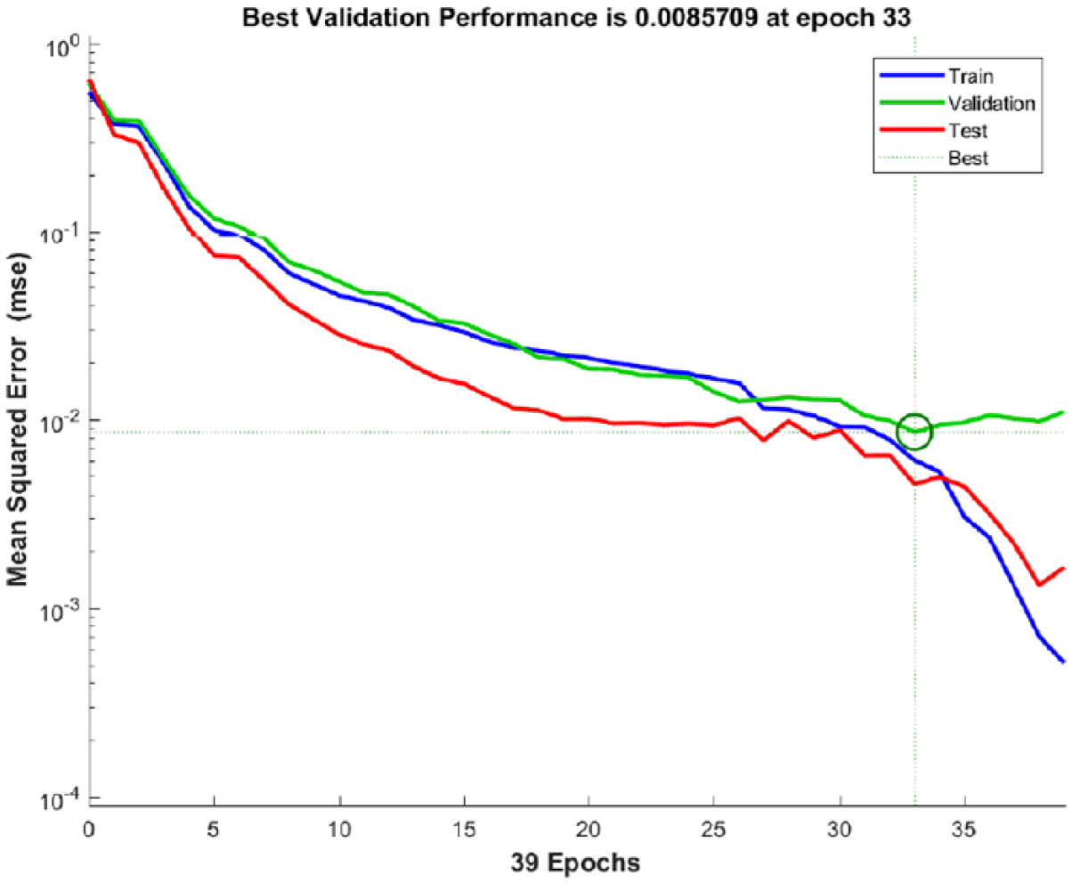
Training performance of the MLP with two hidden layers of 8 and 4 neurons using norm entropy.

V. Conclusion

An approach for defining an engine speed–independent acoustic signature for vehicles is presented. Wavelet packet analysis is chosen as the analysis tool and is explored for different wavelet bases at various depths. Daubechies db4 mother wavelet function is found to give the best classification accuracy at depth 5. Wavelet packet subimages are analyzed further using three features: norm entropy, log energy entropy, and energy. These features are evaluated for their classification accuracy using an MLP as a classifier, and norm entropy is found to give the best result of 100% classification rate with p = 1.1, which is defined by a search in the interval (1, 2). Using final nodes of the WPD provides better results than using all of the nodes. Best-performing MLP is found by pruning the neural network until two hidden layers of eight and four neurons. Future work would be to extend analysis to higher number of vehicles with a wider range of vehicle types including heavy trucks. Moreover, reduction in the feature vector space can be considered in order to decrease complexity of the method. The current results show that under varying engine speeds in the interval between 800 and 3000 r/min, the method of using wavelet packet analysis followed by norm entropy and multilayer perceptron provides an accurate acoustic signature for vehicles independent of the engine speed.

Footnotes

Acknowledgements

The author would like to thank Mr Muammer Göksu, Mr Mustafa Turgut, and Ms Azize Yasemin Göksu Erol for making their vehicles available for measurements of this manuscript.

Funding

The author(s) received no financial support for the research, authorship, and/or publication of this article.

ORCID iD

Hüseyin Göksu

References

Mazarakis

Avaritsiotis

JN.

Vehicle classification in sensor networks using time-domain signal processing and neural networks. Microprocessors and Microsystems 2007; 31(6): 381–92.

Paulraj

Adom

Sundararaj

Classification of moving vehicle using multi-frame time domain features. In 2013 7th international conference on intelligent systems and control (ISCO), Coimbatore, India, 4–5 January 2013, pp.529–33. New York: IEEE.

Wang

Zhou

Vehicle type recognition in WSN based on ITESP algorithm. In 2013 IEEE 10th international conference on ubiquitous intelligence and computing and 10th international conference on autonomic and trusted computing (UIC/ATC), Vietri sul Mere, 18–21 December 2013, pp.668–71. New York: IEEE.

Rahim

Paulraj

Adom

AH.

Classification of moving vehicles using multi-classifier with time-domain approach. International Journal of Computer Applications 2013; 71(1): 12–17.

Paulraj

Adom

Sundararaj

Rahim

NBA

. Moving vehicle recognition and classification based on time domain approach. Procedia Engineering 2013; 53: 405–10.

Mayvan

Beheshti

Masoom

MH.

Classification of vehicles based on audio signals using quadratic discriminant analysis and high energy feature vectors. International Journal on Soft Computing 2015; 6(1): 53–64.

Ishida

Liu

Mimura

Tagashira

Fukuda

Design of acoustic vehicle count system using DTW. In 23rd World Congress of Intelligent Transport Systems, Melbourne, Australia, 10–14 October 2016, pp.1–10. Australia: ITS. Available online at https://www.f.ait.kyushu-u.ac.jp/~ishida/archives/ishida16_its-world.pdf

Nooralahiyan

Dougherty

McKeown

Kirby

HR.

A field trial of acoustic signature analysis for vehicle classification. Transportation Research Part C: Emerging Technologies 1997; 5(3): 165–77.

Siegel

Khosla

Vehicle sound signature recognition by frequency vector principal component analysis. In IEEE instrumentation and measurement technology conference, 1998. IMTC/98. Conference proceedings, St. Paul, MN, 18–21 May 1998, vol. 1, pp.429–34. New York: IEEE.

10.

Nooralahiyan

Kirby

McKeown

Vehicle classification by acoustic signature. Mathematical and Computer Modelling 1998; 27(9–11): 205–14.

11.

Munich

ME.

Bayesian subspace methods for acoustic signature recognition of vehicles. In 2004 12th European Signal Processing Conference, Vienna, 6–10 September 2004, pp.2107–10. New York: IEEE.

12.

Sun

Daigle

JN.

A PCA-based vehicle classification system in wireless sensor networks. In IEEE wireless communications and networking conference, 2006. WCNC 2006, Las Vegas, NV, 3–6 April 2006, vol. 4, pp.2193–8. New York: IEEE.

13.

Yang

Kim

Choi

Vehicle identification using wireless sensor networks. In IEEE SoutheastCon, 2007. Proceedings, Richmond, VA, 22–25 March 2007, pp.41–6. New York: IEEE.

14.

Malhotra

Nikolaidis

Harms

Distributed classification of acoustic targets in wireless audio-sensor networks. Computer Networks 2008; 52(13): 2582–93.

15.

Yang

Kim

Choi

Vehicle identification using discrete spectrums in wireless sensor networks. Journal of Networks 2008; 3(4): 51–63.

16.

Dibazar

Berger

TW.

Noise-robust acoustic signature recognition using nonlinear Hebbian learning. Neural Networks 2010; 23(10): 1252–63.

17.

Dibazar

Berger

TW.

Perimeter security on detecting acoustic signature of approaching vehicle using nonlinear neural computation. In 2008 IEEE conference on technologies for homeland security, Waltham, MA, 12–13 May 2008, pp.51–6. New York: IEEE.

18.

Malhotra

Nikolaidis

Nascimento

MA.

Distributed and efficient classifiers for wireless audio-sensor networks. In 5th international conference on networked sensing systems, 2008. INSS 2008, Kanazawa, Japan, 17–19 June 2008, pp.203–6. New York: IEEE.

19.

Guo

Nixon

Damarla

TR.

Acoustic information fusion for ground vehicle classification. In 2008 11th international conference on information fusion, Cologne, 30 June–3 July 2008, pp.1–7. New York: IEEE.

20.

Bikdash

Kozhisseri

Tettey

Features for the classification of civilian vehicles from acoustic data. US Army RDECOM under contract W911QX-07-C-0062, 2008.

21.

Malhotra

Nikolaidis

Harms

A simple vehicle classification framework for wireless audio-sensor networks. Journal of Telecommunications and Information Technology 2008; 1: 43–50.

22.

Kozhisseri

Bikdash

Spectral features for the classification of civilian vehicles using acoustic sensors. In IEEE workshop on computational intelligence in vehicles and vehicular systems, 2009. CIVVS’09, Nashville, TN, 30 March–2 April 2009, pp.93–100. New York: IEEE.

23.

Changjun

Yuzong

The research of vehicle classification using SVM and KNN in a ramp. In International forum on computer science-technology and applications, 2009. IFCSTA’09, Chongqing, China, 25–27 December 2009, vol. 3, pp.391–4. New York: IEEE.

24.

Rahim

Paulraj

Adom

Sundararaj

Moving vehicle noise classification using backpropagation algorithm. In 2010 6th international colloquium on signal processing and its applications (CSPA), Mallaca City, Malaysia, 21–23 May 2010, pp.1–6. New York: IEEE.

25.

Özgündüz

Türkmen

Hİ

Şentürk

Karslıgil

Yavuz

AG.

Vehicle identification using acoustic and seismic signals. In 2010 IEEE 18th signal processing and communications applications conference (SIU), Diyarbakir, 22–24 April 2010, pp.941–4. New York: IEEE.

26.

Mato-Méndez

Sobreira-Seoane

MA.

Detecting multiple simultaneous vehicles pass-by sound source separation techniques. In INTER-NOISE and NOISE-CON congress and conference proceedings, Lisbon, Portugal, 13–16 June 2010, vol. 2010, no. 8, pp.3142–50. Reston, VA: Institute of Noise Control Engineering.

27.

Zhao

Yan

Wang

Tang

Chai

Recognition of Mill Load with KPCA and KNN Based on Shell Vibration Signals. In 2011 3rd international workshop on intelligent systems and applications (ISA), Wuhan, China, 28–29 May 2011, pp.1–4. New York: IEEE.

28.

Bhave

Rao

Vehicle engine sound analysis applied to traffic congestion estimation. In Proceedings of 8th International Symposium, CMMR 2011 and 20th International Symposium, FRSM 2011, Bhubaneswar, India, 9–12 March 2011, pp.59–63. Available online at https://www.ee.iitb.ac.in/student/~daplab/publications/nikhil-pr-frsm-2011.pdf

29.

Górski

Zarzycki

Feature extraction in vehicle classification. In 2012 international conference on signals and electronic systems (ICSES), Wroclaw, 18–21 September 2012, pp.1–6. New York: IEEE.

30.

Guo

Nixon

Damarla

Improving acoustic vehicle classification by information fusion. Pattern Analysis and Applications 2012; 15(1): 29–43.

31.

Rahim

Paulraj

Adom

AH.

Adaptive boosting with SVM classifier for moving vehicle classification. Procedia Engineering 2013; 53: 411–9.

32.

Biernacki

Acoustic information fusion for vehicles identification. In 2014 19th international conference on methods and models in automation and robotics (MMAR), Miedzyzdroje, 2–5 September 2014, pp.711–5. New York: IEEE.

33.

Zambon

Roman

Benocci

Scaling model for a speed-dependent vehicle noise spectrum. Journal of Traffic and Transportation Engineering 2017; 4: 230–9.

34.

Sunu

Percus

AG.

Dimensionality reduction for acoustic vehicle classification with spectral clustering. arXiv preprint arXiv:1705.09869, 2017.

35.

Zambon

Roman

Benocci

Vehicle speed recognition from noise spectral patterns. International Journal of Environmental Research 2017; 11: 449–59.

36.

Averbuch

Hulata

Zheludev

Kozlov

A wavelet packet algorithm for classification and detection of moving vehicles. Multidimensional Systems and Signal Processing 2001; 12(1): 9–31.

37.

Dibazar

Berger

TW.

Nonlinear Hebbian learning for noise-independent vehicle sound recognition. In IEEE international joint conference on neural networks, 2008. IJCNN 2008 (IEEE World Congress on Computational Intelligence), Hong Kong, China, 1–8 June 2008, pp.1336–43. New York: IEEE.

38.

Averbuch

Zheludev

Rabin

Schclar

Wavelet-based acoustic detection of moving vehicles. Multidimensional Systems and Signal Processing 2009; 20(1): 55–80.

39.

Schclar

Averbuch

Rabin

Zheludev

Hochman

A diffusion framework for detection of moving vehicles. Digital Signal Processing 2010; 20(1): 111–22.

40.

Aljaafreh

Dong

An evaluation of feature extraction methods for vehicle classification based on acoustic signals. In 2010 international conference on networking, sensing and control (ICNSC), Chicago, IL, 10–12 April 2010, pp.570–5. New York: IEEE.

41.

Padmavathi

Shanmugapriya

Kalaivani

Neural network approaches and MSPCA in vehicle acoustic signal classification using wireless sensor networks. In 2010 IEEE international conference on communication control and computing technologies (ICCCCT), Ramanathapuram, India, 7–9 October 2010, pp.372–6. New York: IEEE.

42.

Aljaafreh

Al-Fuqaha

Multi-target classification using acoustic signatures in wireless sensor networks: A survey. Signal Processing: An International Journal 2010; 4(4): 175.

43.

George

Cyril

Koshy

Mary

Exploring sound signature for vehicle detection and classification using ANN. International Journal on Soft Computing 2013; 4(2): 29.

44.

Kakar

Kandpal

Techniques of acoustic feature extraction for detection and classification of ground vehicles. International Journal of Emerging Technology and Advance Engineering 2013; 3(2): 419–26.

45.

Shah

Mehta

PD.

Analysis of acoustic signals for vehicle classification of four wheeler models using feature extraction methods. In Recent advances and innovations in engineering (ICRAIE), 2014, Jaipur, India, 9–11 May 2014, pp.1–4. New York: IEEE.

46.

Wickerhauser

MV.

Adapted Wavelet Analysis from Theory to Software. Piscataway, NJ: IEEE Press, 1994.

47.

Yen

Lin

KC.

Wavelet packet feature extraction for vibration monitoring. IEEE Transactions on Industrial Electronics 2000; 47(3): 650–67.

48.

Liu

CH.

An expert system for fault diagnosis in internal combustion engines using wavelet packet transform and neural network. Expert Systems with Applications 2009; 36(3): 4278–86.

49.

Akansu

Haddad

RA.

Multiresolution Signal Decomposition: Transforms, Subbands, and Wavelets. New York: Academic Press, 2001.

50.

Lippmann

RP.

Pattern classification using neural networks. IEEE Communications Magazine 1989; 27(11): 47–50.

51.

Roth

MW.

Survey of neural network technology for automatic target recognition. IEEE Transactions on Neural Networks 1990; 1(1): 28–43.

52.

Chauvin

Rumelhart

(eds). Backpropagation: Theory, Architectures, and Applications. Abingdon: Psychology Press, 1995.

53.

Wang

McFadden

PD.

Application of orthogonal wavelets to early gear damage detection. Mechanical Systems and Signal Processing 1995; 9(5), 497–507.

Engine Speed–Independent Acoustic Signature for Vehicles

Abstract

Keywords

I. Introduction

II. Material

III. Method

A. WPD

B. Feature

C. Classifier: MLP

IV. Results and Discussion

V. Conclusion

Footnotes

Acknowledgements

Funding

ORCID iD

References