Sage Journals: Discover world-class research

Abstract

Estimation of vehicle speed by analysis of drive-by noise is a known technique. The methods used in this kind of practice generally estimate the velocity of the vehicle with respect to the microphone(s), so they rely on the relative motion of the vehicle to the microphone(s). There are also other methods that do not rely on this technique. For example, recent research has shown that there is a statistical correlation between vehicle speed and drive-by noise emissions spectra. This does not rely on the relative motion of the vehicle with respect to the microphone(s) so it inspires us to consider the possibility of predicting velocity of the vehicle using an on-board microphone. This has the potential for the development of a new kind of speed sensor. For this purpose we record sound signal from a vehicle under speed variation using an on-board microphone. Sound emissions from a vehicle are very complex, which is from the engine, the exhaust, the air conditioner, other mechanical parts, tires, and air resistance. These emissions carry both stationary and non-stationary information. We propose to make the analysis by wavelet packet analysis, rather than traditional time or frequency domain methods. Wavelet packet analysis, by providing arbitrary time-frequency resolution, enables analyzing signals of stationary and non-stationary nature. It has better time representation than Fourier analysis and better high-frequency resolution than Wavelet analysis. Subsignals from the wavelet packet analysis are analyzed further by Norm Entropy, Log Energy Entropy, and Energy. These features are evaluated by feeding them into a multilayer perceptron. Norm entropy achieves the best prediction with 97.89% average accuracy with 1.11 km/h mean absolute error which corresponds to 2.11% relative error. Time sensitivity is ±0.453 s and is open to improvement by varying the window width. The results indicate that, with further tests at other speed ranges, with other vehicles and under dynamic conditions, this method can be extended to the design of a new kind of vehicle speed sensor.

Keywords

Vehicles sound emission speed measurement wavelet packet analysis entropy multilayer perceptron

Introduction

A vehicle can produce a complex sound emission from its engine, the exhaust, the air conditioner, tires, other mechanical systems, and air friction. The possibility of making diagnosis or identification of vehicles based on sound emission analysis has been investigated by researchers.

An important parameter in the vehicle noise emission is vehicle speed. Speed estimation by analyzing drive-by noise of vehicles has been investigated by researchers. Some of these techniques are based on Doppler shift,¹ which depends on the relative motion of the vehicle with respect to the receiver microphone. There are a few other techniques that use signals from microphone arrays and/or omnidirectional microphones^2–6 which also rely on the relative motion of the vehicle with respect to the receiver microphone(s). Although still using drive-by noise of the vehicles, there are a few other techniques that do not rely on the relative motion of the vehicle with respect to the microphone.^7–9 Recently, Zambon et al.⁷ used a database of vehicles to statistically analyze 1/3-octave band spectra of emission noise in terms of its relevance to vehicle speed and used recorded spectra of vehicles to detect a statistical correlation between the vehicle speed and noise spectra.⁸ Their method does not rely on the relative motion of the vehicle with respect to the microphone(s). So this inspires us to consider the possibility of using a similar method to estimate the speed of a vehicle using sound signals recorded from an on-board microphone. This may result in a new kind of speed sensor.

Identification, diagnosis, and parameter estimation of vehicles based on the analysis of sound emissions has been investigated by researchers. Various methods have been proposed for these analysis. Below is a chronological review of time-domain, frequency-domain, time–frequency domain, and hybrid analysis methods used in vehicle acoustic signal analysis.

Some of the researchers used time-domain features, for example, Mazarakis and Avaritsiotis¹⁰ used a time-domain encoding and feature extraction to classify tracked vehicles and heavy trucks using their acoustic and seismic signatures; Paulraj et al.¹¹ used multi-frame time-domain features for classification of moving vehicles; Wang and Zhou¹² used an improved time-encoded signal-processing algorithm for feature extraction in acoustic vehicle-type recognition; Rahim et al.¹³ used time-domain features for the classification of moving vehicles; Paulraj et al.¹⁴ used autoregressive modeling for vehicle-type classification; Mayvan et al.¹⁵ used quadratic discriminant analysis to classify audio signals of passing vehicles to bus, car, motor, and truck categories based on features such as short-time energy, average zero-crossing rate, and pitch frequency of periodic segments of signals; and Ishida et al.¹⁶ used dynamic time warping to design an acoustic vehicle-count system.

Some of the researchers used frequency-domain features, for example, Nooralahiyan et al.¹⁷ used linear predictive coding coefficients, auditory model processing, and Fourier transform for acoustic signature analysis for vehicle classification; Wu et al.¹⁸ used frequency vector principal component analysis for vehicle sound signature recognition; Nooralahiyan et al.¹⁹ used linear predictive coding for vehicle classification by acoustic signature; Munich²⁰ used a probabilistic classifier that is trained on the principal components subspace of the short-time Fourier transform for acoustic signature recognition of vehicles; Sun and Daigle²¹ used fast Fourier transform (FFT) magnitudes for vehicle classification; Yang et al.²² used overall shape of sound spectrum for vehicle identification; Malhotra et al.²³ used features based on FFT and power spectral density (PSD) to classify running vehicles; Yang et al.²⁴ used discrete spectrums to identify vehicles in wireless sensor networks; Lu et al.²⁵ used spectral features to classify running vehicle types into gasoline light-wheeled, gasoline heavy-wheeled, diesel truck, and motorcycle; Lu et al.²⁶ used gammatone filterbanks as spectral features for detecting acoustic signature of approaching vehicles; Malhotra et al.²⁷ used PSD-based features for classifications in audio-sensor networks; Guo et al.²⁸ used a number of harmonic components and a group of key frequency components for ground vehicle classification; Bikdash et al.²⁹ used tristimulus response for classification of civilian vehicles from acoustic data; Malhotra et al.³⁰ used Aura matrices to create a new feature derived from the PSD and dynamic multidimensional PSD for vehicle classification by wireless audio-sensor networks; Kozhisseri and Bikdash³¹ used spectral features for the classification of civilian vehicles using acoustic sensors; Changjun and Yuzong³² used short-time Fourier transform of acoustic and seismic signals for vehicle classification; Rahim et al.³³ used one-third octave filter bands for moving vehicle noise classification; Özgündüz et al.³⁴ used Mel-frequency cepstral coefficients for vehicle identification using acoustic and seismic signals; Mato-Méndez and Sobreira-Seoane³⁵ used Mel-frequency cepstral coefficients, sub-band energy ratio, spectral centroid, and spectral roll-off point to classify vehicles; Zhao et al.³⁶ used PSD to recognize status of ball mill load using shell vibration signal; Bhave and Rao³⁷ used formant-based feature and Mel-frequency cepstral coefficients for vehicle engine sound analysis applied to traffic congestion estimation; Górski and Zarzycki³⁸ used Harmonic line, Shur coefficients, and Mel filters methods for feature extraction in acoustic vehicle classification; Guo et al.³⁹ used a number of harmonic components and a group of key frequency components for ground vehicle classification; Rahim et al.⁴⁰ used one-third octave filter band for moving vehicle classification; Rahim et al.⁴⁰ used one-third octave frequency spectrum analysis to classify type and the distance of a moving vehicle with types: car, bike, lorry, and truck; Biernacki⁴¹ used harmonic features and correlation features for acoustic vehicle identification; Zambon et al.⁷ used a database of vehicles to statistically analyze one-third octave band spectra of emission noise in terms of its relevance to vehicle speed; Sunu and Percus⁴² used frequency signatures to classify vehicles; and Zambon et al.⁸ used statistical analysis of recorded spectra of vehicles to detect its relevance to vehicle speed.

Some of the researchers used time–frequency domain features, for example, Averbuch et al.⁴³ used wavelet packet energy for the classification and detection of moving vehicles; Lu et al.⁴⁴ assembled gammatone feature vectors over multiple temporal frames to establish a high-dimensional spectro-temporal representation for noise-independent vehicle sound recognition; Averbuch et al.⁴⁵ used energy of wavelet packet transform (WPT) for acoustic detection of moving vehicles; and Schclar et al.⁴⁶ used total magnitude (L1 norm) of the coefficients from wavelet packet decomposition (WPD) to detect vehicles.

Some of the researchers used hybrid features, for example, Aljaafreh and Dong⁴⁷ used PSD of short-time Fourier spectrum and energy of WPT for vehicle classification based on acoustic signals; Padmavathi et al.⁴⁸ used signal energy, energy entropy, zero-crossing rate, spectral roll-off, spectral centroid, and spectral flux for vehicle acoustic signal classification; Aljaafreh and Al-Fuqaha⁴⁹ used spectrum analysis and energy of WPT for acoustic classification of multiple targets; George et al.⁵⁰ used short-time energy, log energy, and smoothed log energy for vehicle detection and Mel-frequency cepstral coefficients for vehicle classification; Kakar and Kandpal⁵¹ reviewed time-domain, frequency-domain, and time–frequency domain feature extraction methods that are used in classification of vehicles; and Shah and Mehta⁵² used time-domain and frequency-domain features for the analysis of acoustic signals for vehicle classification of four-wheeler models.

Time domain, frequency domain (Fourier), and time–frequency domain (Wavelet) analysis are the main tools for analyzing signals but Fourier analysis has poor time representation, and wavelet analysis has poor resolution at high frequency. Wavelet packet analysis (WPA), on the other hand, overcomes both of these, and the arbitrary time–frequency resolution enables analysis of signals of stationary and non-stationary nature.

In this work, we would like to predict the speed of a vehicle based on the analysis of its sound emissions recorded from an on-board microphone. For this purpose, we record sound of a vehicle by varying and recording its speed. For its aforementioned advantages, we choose to make the analysis by WPA. Output of the WPA is a set of subsignals whose number depends on the depth of the WPA. From these subsignals, we extract several features including Energy, Log Energy Entropy, and Norm Entropy. We evaluate these features and choose whichever results in best prediction. To map the feature vectors to vehicle speed, we use a multilayer perceptron (MLP) which is a kind of neural network which is proven to be successful in black box modeling and function approximation. Although, in the past studies, WPA has been used along with energy in vehicle acoustic analysis,^43,45 Entropy is used for the first time by us in vehicle acoustic emission analysis along with WPA in this study.

Material

Sound emissions are recorded from a Ford Kuga 1.5 Ecoboost, using its cruise control to control its speed in 1 km/h increments starting from 30 km/h and going up to 80 km/h. Sound is recorded by placing the microphone inside the vehicle, on the front passenger’s seat, windows closed, and the air conditioner on, which is a significant noise source. Recording is done by a digital recorder at 44,100 Hz for 30 s at each speed step. Recordings from each speed step are partitioned into 40 windows to provide 20 parts for training and 20 parts for testing for each speed step. A total of 475 sets of training and 475 for testing is obtained. Figure 1 displays one set of data from each of 30, 40, 50, 60, 70, and 80 km/h speed steps. Since each window is 0.907 s long, we have a time sensitivity of ±0.453 s.

Figure 1.

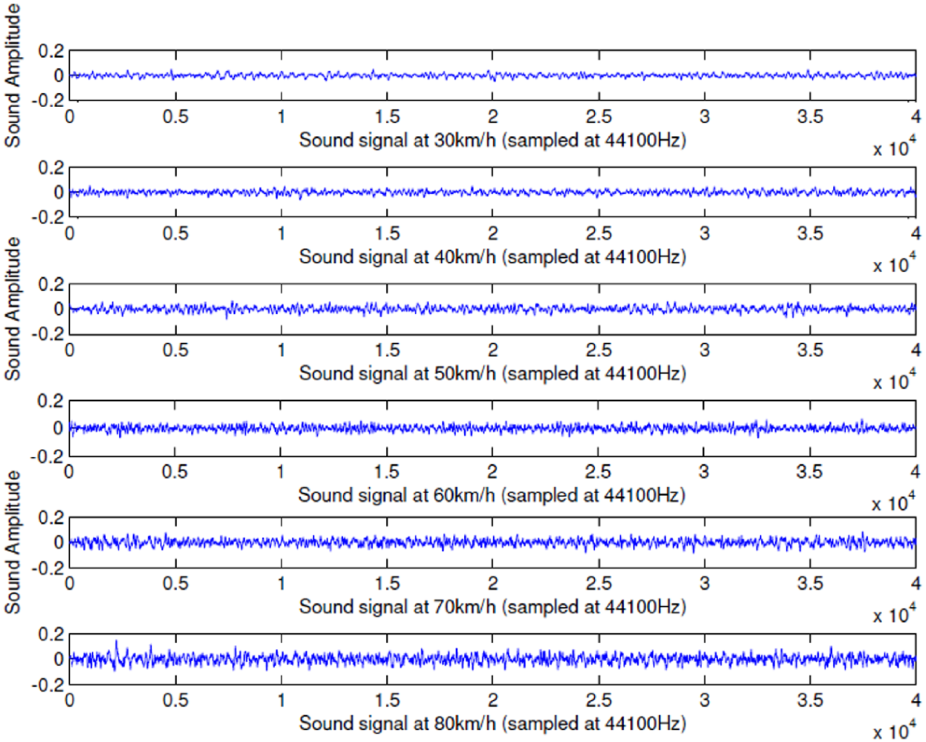
Sound signals recorded at speeds 30, 40, 50, 60, 70, and 80 km/h.

Method

Our analysis and prediction workflow is such that each signal is first decomposed into wavelet packet subsignals using WPA. Then, features are extracted from these subsignals in the form of Norm Entropy, Log Energy Entropy, and Energy. To select best of these features, we feed them into the prediction tool, the MLP, to further fine tune the parameters: WPA depth, mother wavelet, and which nodes (all or final) of WPA to include in the prediction and the neural network parameters. After this step, we analyze the contribution of each component of the feature vector which corresponds to the nodes of WPA by a plot of mean of the feature vectors at different speed steps and then box plot the features at each of the nodes for varying speeds. These results let us decide whether further reduction in the feature space or fine-tuning of the parameters is needed.

WPD

WPD is used to decompose the signals. Wavelet packets are a generalization of wavelet bases by taking linear combinations of wavelet functions.⁵³ In the following explanation, we take a parallel approach to Yen and Lin⁵⁴ and Wu and Liu.⁵⁵

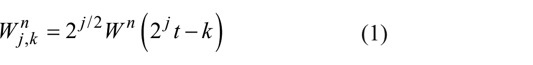
A wavelet function has three indices, j: index scale (integer), k: translation (integer), n: oscillation parameter; and t is time

W_{j, k}^{n} = 2^{j / 2} W^{n} (2^{j} t - k)

(1)

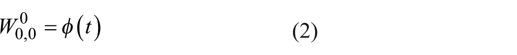
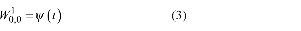
The first two wavelet packet functions are a scaling function and the mother wavelet function

W_{0, 0}^{0} = ϕ (t)

(2)

W_{0, 0}^{1} = ψ (t)

(3)

Wavelet packet functions with higher oscillation parameters are

W_{0, 0}^{2 n} = \sqrt{2} \sum_{k} h (k) W_{1, k}^{n} (2 t - k)

(4)

W_{0, 0}^{2 n + 1} = \sqrt{2} \sum_{k} g (k) W_{1, k}^{n} (2 t - k)

(5)

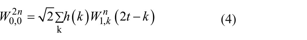
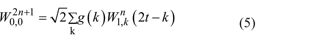
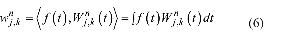
where h(k) and g(k) are quadrature mirror filters⁵⁶ associated with the scaling function and the mother wavelet function. The wavelet packet coefficients are defined as the inner product of wavelet packet functions with the input signal f(t), which also defines the range of t

w_{j, k}^{n} = 〈 f (t), W_{j, k}^{n} (t) 〉 = \int^{​} f (t) W_{j, k}^{n} (t) d t

(6)

WPD is applied as shown in Figure 2 for three levels. The left-hand side sub-branches are obtained by low pass filter h(k) and decimation; the right-hand side sub-branches are obtained by high pass filter g(k) and decimation. S is the original signal, A stands for approximation, and D for detail and the number for level.

Figure 2.

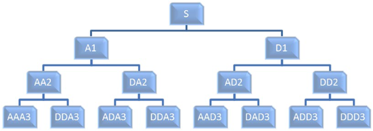
WPD tree up to three levels.

Features

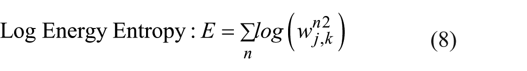
Norm Entropy, Log Energy Entropy, and Energy are used as feature vectors for prediction. Entropy and energy are common measures used in signal processing which are able to extract useful information from a signal

Norm Entropy : E = \sum_{n} {| w_{j, k}^{n} |}^{p}

(7)

Log Energy Entropy : E = \sum_{n} l o g (w_{j, k}^{n 2})

(8)

Energy : E = \sum_{n} w_{j, k}^{n 2}

(9)

where $w_{j, k}^{n}$ are the WPD coefficients calculated in equation (6) and 1 ≤ p.

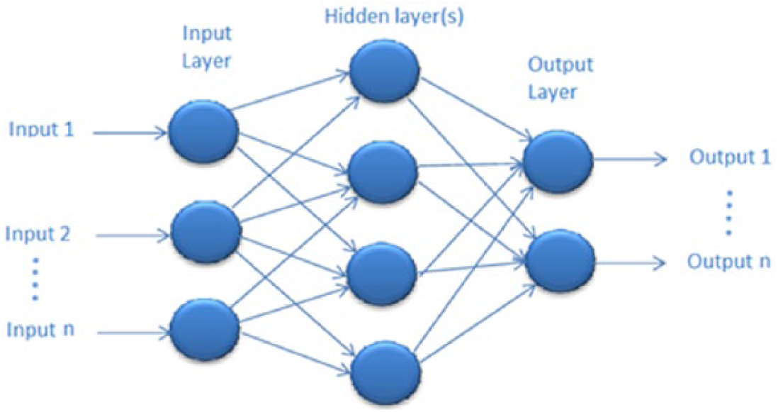
Predictor: MLP

We choose MLP with backpropagation learning which can efficiently process large datasets and has been shown to be effective in black box modeling and function approximation.^57,58

MLP is a network of nodes arranged in layers. A node can be modeled as an artificial neuron that computes weighted sums of inputs with bias and presents it to an activation function. A general MLP model is shown in Figure 3.

Figure 3.

General architecture of the MLP.

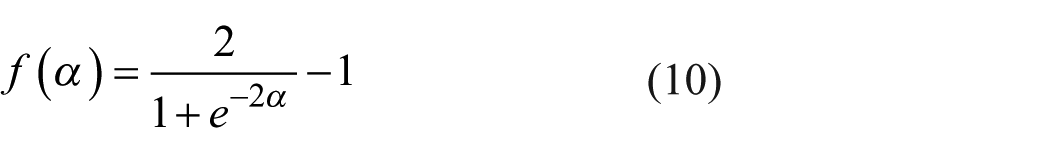
Linear activation functions are used for input and output layers and hyperbolic tangent sigmoid activation function for the hidden layer(s) which are in the form

f (α) = \frac{2}{1 + e^{- 2 α}} - 1

(10)

where $α$ is the input to the neuron. Training of the MLP is the adjustment of the weight parameters to map the Input to the Output with minimum error. For this purpose, backpropagation algorithm is adopted where the error between the actual output of the network and the target is backpropagated through the network to adjust the weight parameters.^59,60

Results and discussion

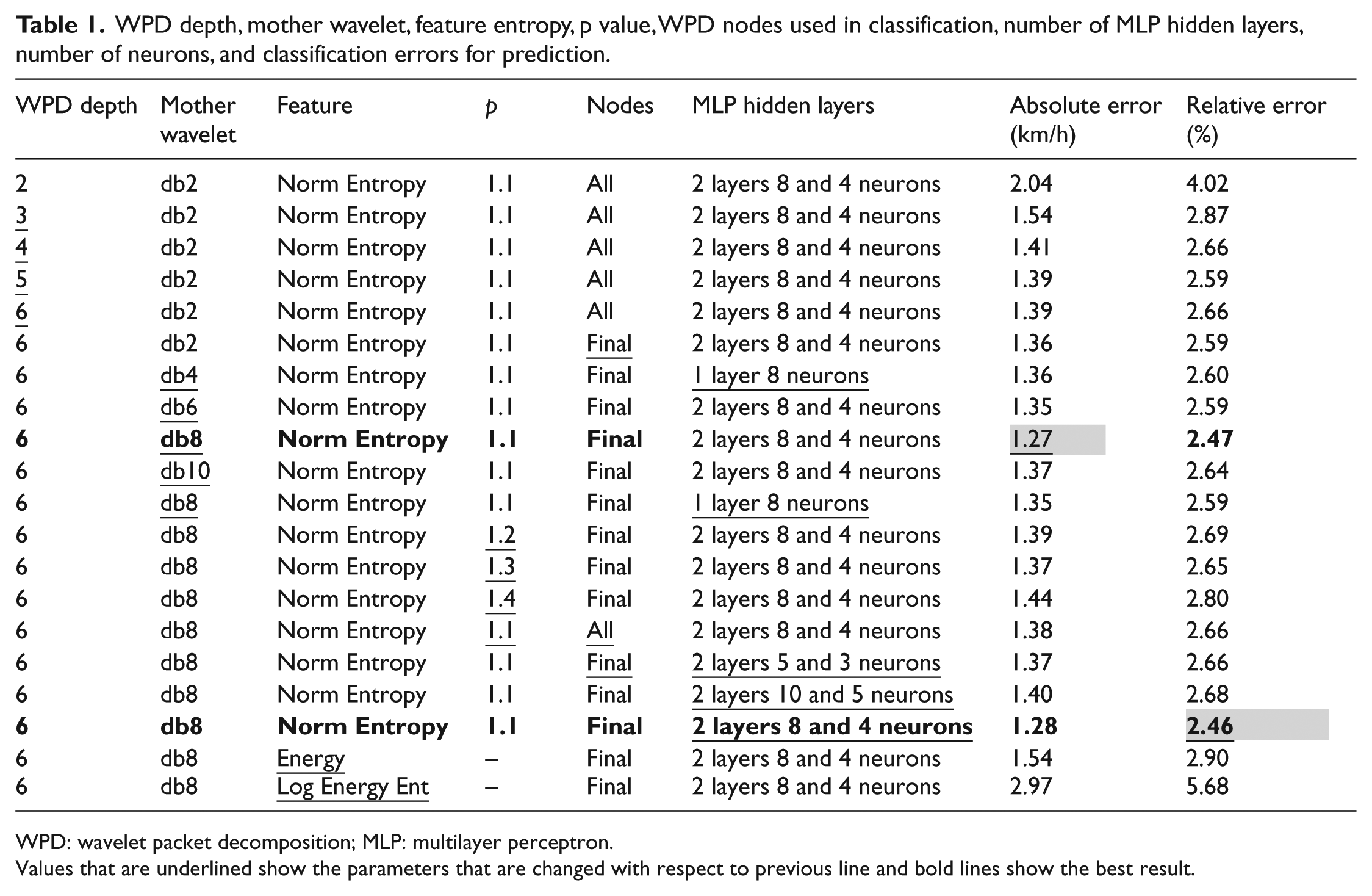
We start by WPD of the signals. We start with Daubechies db2 as our mother wavelet and search the Daubechies family looking for best prediction accuracy. Level of the WPD is determined by a search starting with 2 and increasing until best prediction accuracy. We include all nodes of the WPD up to the final level and then switch to using only the final nodes which gives better prediction accuracy. We use Log Energy Entropy, Energy, and Norm Entropy as feature vectors and see that Norm Entropy gives best prediction accuracy with parameter p = 1.1, which is found by a search in the interval (1, 2). Neural network parameters, which are the number of hidden layers and number of neurons, are determined by pruning. This is to start with the simplest network of 1 hidden layer of 1 neuron and increasing complexity until best prediction accuracy. WPD depth is increased one step at a time until level 6, which gives the best accuracy. The WPD subsignals of the final nodes at depth 6 corresponding to V = 30 km/h and V = 60 km/h are shown in Figure 4. Each horizontal line in this figure is a subsignal. Visually it is not easy to differentiate between the subsignals under speed variation.

Figure 4.

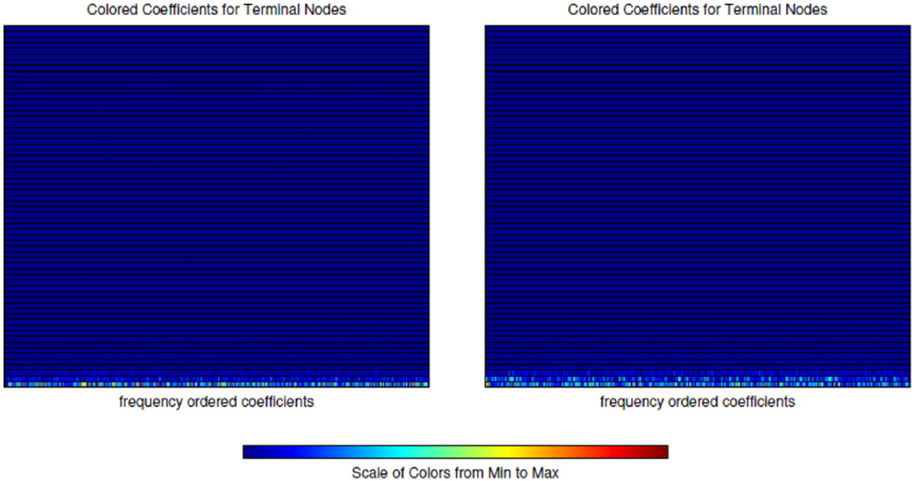
WPD subsignals of final nodes at level 6 for V = 30 km/h (left) and V = 60 km/h (right).

The search we perform in the parameter spaces is given in Table 1. Underlined values show the parameter that is changed with respect to the previous line. As we can see, Norm Entropy achieves the best result with a mean absolute prediction error of 1.27 km/h which corresponds to a relative error of 2.46%. The parameters that correspond to this best prediction are given in Table 1. From our earlier experience in similar applications, we have seen that if Energy, Log Energy Entropy, and Norm Entropy are compared in terms of classification or prediction accuracy at one set of parameters, the one that performs the best in that set of parameters continue to perform the best at other parameter values. Or if the parameters are optimized using one of these features, it means they are optimized for all three features. Therefore, in our search listed in Tables 1 and 2, once we optimized the parameters using Norm Entropy, it means we have optimized the parameters for all three features; afterward we try Log Energy Entropy and Energy, and since we see that Norm Entropy performs the best, we continue with it in the rest of the study.

Table 1.

WPD depth, mother wavelet, feature entropy, p value, WPD nodes used in classification, number of MLP hidden layers, number of neurons, and classification errors for prediction.

WPD depth	Mother wavelet	Feature	p	Nodes	MLP hidden layers	Absolute error (km/h)	Relative error (%)
2	db2	Norm Entropy	1.1	All	2 layers 8 and 4 neurons	2.04	4.02
3	db2	Norm Entropy	1.1	All	2 layers 8 and 4 neurons	1.54	2.87
4	db2	Norm Entropy	1.1	All	2 layers 8 and 4 neurons	1.41	2.66
5	db2	Norm Entropy	1.1	All	2 layers 8 and 4 neurons	1.39	2.59
6	db2	Norm Entropy	1.1	All	2 layers 8 and 4 neurons	1.39	2.66
6	db2	Norm Entropy	1.1	Final	2 layers 8 and 4 neurons	1.36	2.59
6	db4	Norm Entropy	1.1	Final	1 layer 8 neurons	1.36	2.60
6	db6	Norm Entropy	1.1	Final	2 layers 8 and 4 neurons	1.35	2.59
6	db8	Norm Entropy	1.1	Final	2 layers 8 and 4 neurons	1.27	2.47
6	db10	Norm Entropy	1.1	Final	2 layers 8 and 4 neurons	1.37	2.64
6	db8	Norm Entropy	1.1	Final	1 layer 8 neurons	1.35	2.59
6	db8	Norm Entropy	1.2	Final	2 layers 8 and 4 neurons	1.39	2.69
6	db8	Norm Entropy	1.3	Final	2 layers 8 and 4 neurons	1.37	2.65
6	db8	Norm Entropy	1.4	Final	2 layers 8 and 4 neurons	1.44	2.80
6	db8	Norm Entropy	1.1	All	2 layers 8 and 4 neurons	1.38	2.66
6	db8	Norm Entropy	1.1	Final	2 layers 5 and 3 neurons	1.37	2.66
6	db8	Norm Entropy	1.1	Final	2 layers 10 and 5 neurons	1.40	2.68
6	db8	Norm Entropy	1.1	Final	2 layers 8 and 4 neurons	1.28	2.46
6	db8	Energy	–	Final	2 layers 8 and 4 neurons	1.54	2.90
6	db8	Log Energy Ent	–	Final	2 layers 8 and 4 neurons	2.97	5.68

WPD: wavelet packet decomposition; MLP: multilayer perceptron.

Values that are underlined show the parameters that are changed with respect to previous line and bold lines show the best result.

Table 2.

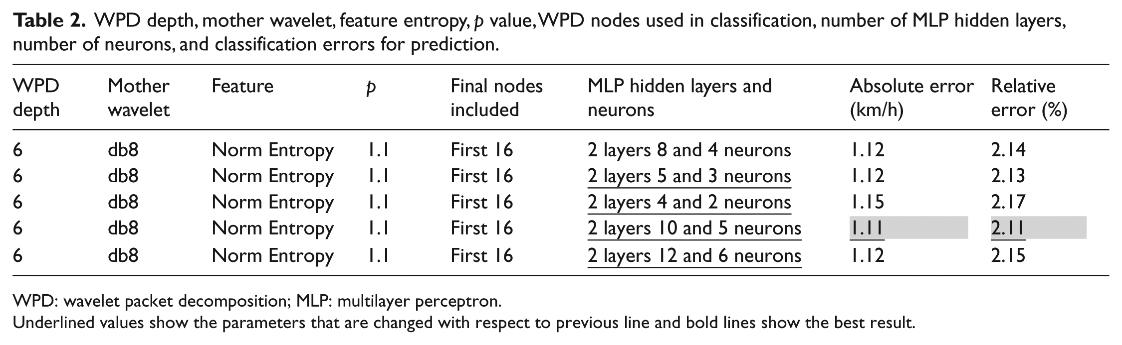
WPD depth, mother wavelet, feature entropy, p value, WPD nodes used in classification, number of MLP hidden layers, number of neurons, and classification errors for prediction.

WPD depth	Mother wavelet	Feature	p	Final nodes included	MLP hidden layers and neurons	Absolute error (km/h)	Relative error (%)
6	db8	Norm Entropy	1.1	First 16	2 layers 8 and 4 neurons	1.12	2.14
6	db8	Norm Entropy	1.1	First 16	2 layers 5 and 3 neurons	1.12	2.13
6	db8	Norm Entropy	1.1	First 16	2 layers 4 and 2 neurons	1.15	2.17
6	db8	Norm Entropy	1.1	First 16	2 layers 10 and 5 neurons	1.11	2.11
6	db8	Norm Entropy	1.1	First 16	2 layers 12 and 6 neurons	1.12	2.15

WPD: wavelet packet decomposition; MLP: multilayer perceptron.

Underlined values show the parameters that are changed with respect to previous line and bold lines show the best result.

To see the contribution of each node to prediction, we first plot mean values of Norm Entropy corresponding to final 64 nodes of WPD until depth 6 for speeds V = 30, 40, 50, 60, 70, and 80 km/h in Figure 5. Visually only several nodes from the first part seem to be contributing to identification by showing variation at different speeds, but it is not easy to see which nodes these are.

Figure 5.

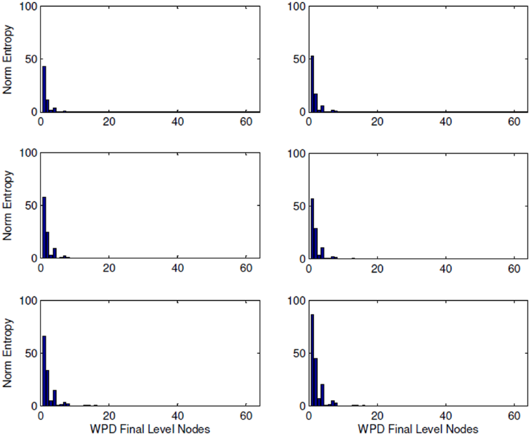
Mean values of Norm Entropy for final 64 nodes of WPD corresponding to vehicle speeds 30, 40, 50, 60, 70, and 80 km/h.

A box plot of norm entropy at each of the nodes at speeds V = 30, 40, 50, 60, 70, and 80 km/h in Figures 6 and 7 shows us exactly which nodes are contributing to prediction. In these figures, the central mark of each box is the median, the edges are the 25th and 75th percentiles, and the whiskers cover the most extreme data points that are not outliers. Outliers are plotted individually as red “+” signs. These plots show that only at the first 16 nodes, speeds are differentiable from each other, therefore only these nodes contribute to prediction. These are the lower frequency nodes. The rest of the nodes with higher frequency show less variation and they overlap with each other under varying speeds so they seem to be useless in prediction. So we decide to continue by keeping only the first 16 nodes among the final nodes of WPD at depth 6 in our analysis.

Figure 6.

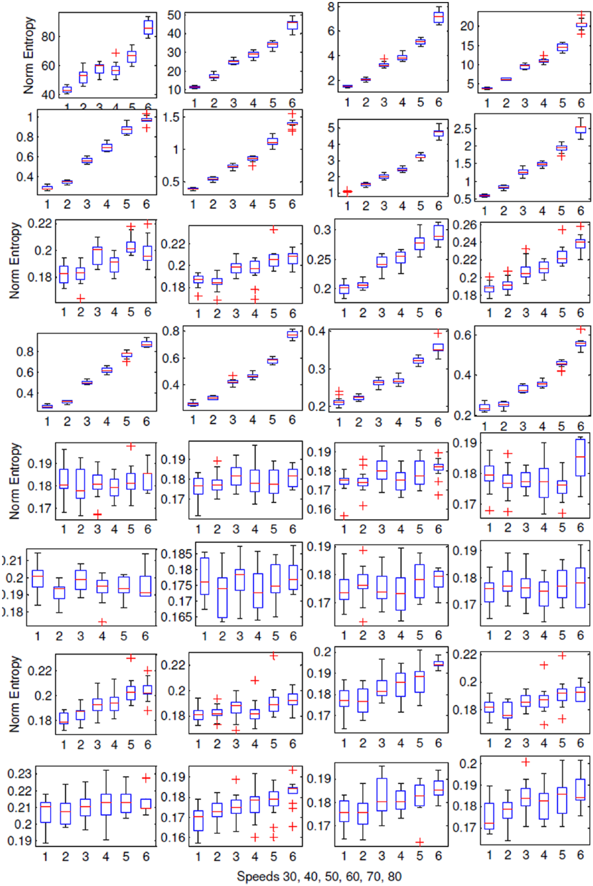
Box plot of Norm Entropy for nodes 1–32 of final nodes of WPD at depth 6 corresponding to vehicle speeds 30, 40, 50, 60, 70, and 80 km/h.

Figure 7.

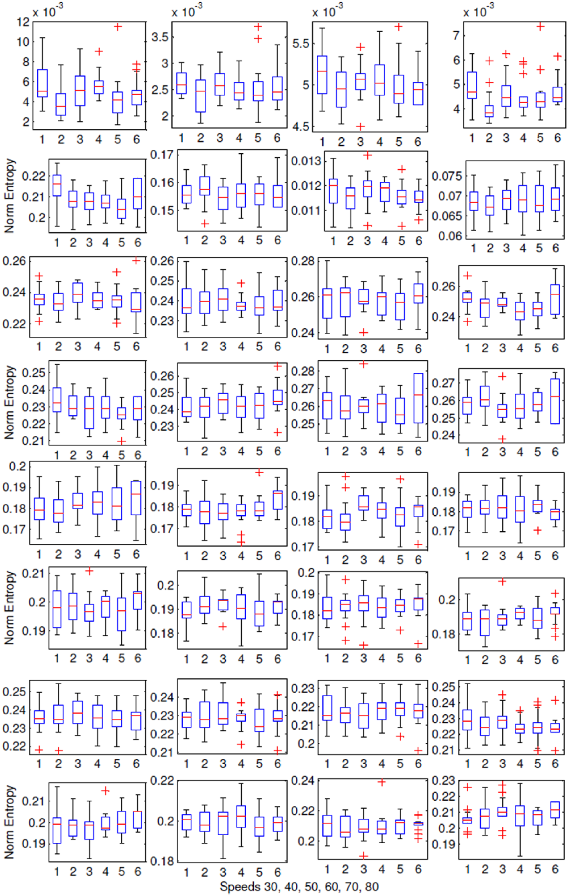
Box plot of Norm Entropy for nodes 33–64 of final nodes of WPD at depth 6 corresponding to vehicle speeds 30, 40, 50, 60, 70, and 80 km/h.

Table 2 shows our results using only the first 16 nodes. We again perform a search in the parameter spaces to fine-tune the parameters. We see that these results are better than the ones in Table 1, which shows that keeping only the first 16 nodes was the right choice. Now since the input size of the MLP has changed, we fine-tune MLP parameters too. We see that we achieve the best prediction with 1.11 km/h mean absolute error and its corresponding 2.11% relative error with MLP with two hidden layers of 10 and 5 neurons. Figure 8 shows the training performance of this final MLP.

Figure 8.

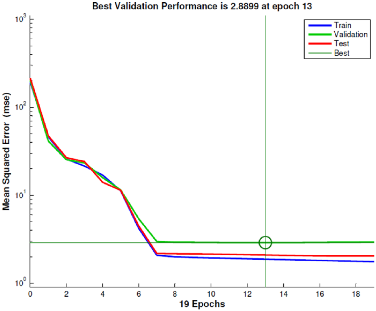
Training performance of the MLP with two hidden layers of 10 and 5 neurons.

Figure 9 shows the prediction results by plotting the actual speeds and predicted speeds for all test instances. We see that prediction is mostly consistent, that is, random fluctuations in prediction are minor. There are fluctuations as a group of neighboring instances which means that there is inaccuracy in the control and measurement of the speed. As we mentioned earlier, speed control and measurement is done using the cruise control of the vehicle. This is a device which tries to keep the speed fixed at a determined value. But as with all control systems, it can control with a certain uncertainty. The road slope variation causes vehicle speed to follow a variable pattern. This shows that if measurement and control could be done more precisely, the method would perform better. Under these conditions, the results indicate that our method is able to predict the speed of the vehicle with 1.11 km/h average absolute error and its corresponding 2.11% relative error with ±0.453 s time sensitivity by sound emission analysis using an on-board microphone. These results are in the speed range between 30 and 80 km/h and they are under steady-state conditions. Testing with other vehicles, at other speed ranges and under dynamic conditions, the method can be extended for the design of a new kind of speed sensor. Speed measurement and control must be done more precisely in these tests. Time sensitivity may also be improved by reducing the window size. The algorithm can be optimized along with the use of a faster CPU. These are to be performed in a future study in order to generalize the method to the design of a new kind of vehicle speed sensor.

Figure 9.

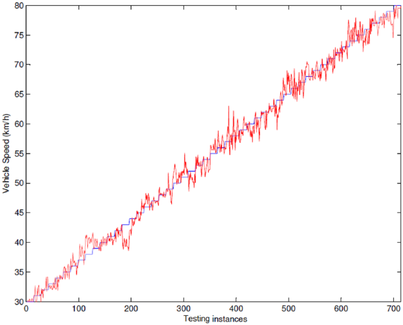
Actual speeds (blue) and predicted speeds (red) for all test instances.

Conclusion

An approach for predicting vehicle speed by sound emission analysis using an on-board microphone is presented. WPD is used as the analysis tool and is explored for different wavelet base functions at various depths. Daubechies db8 mother wavelet is found to give the best result at depth 6. Features of Log Energy Entropy, Norm Entropy, and Energy are explored and Norm Entropy is found to give the best accuracy with p = 1.1. Using the final nodes of the WPD than using all nodes gives better prediction accuracy. Analysis of the variation of Norm Entropy among final nodes shows us that the first 16 nodes, which are the lower frequency nodes, show distinction under varying speed, therefore only these contribute to prediction and we only keep these nodes in the remaining part of the analysis. Fine-tuning of the parameters is finalized by pruning the MLP until two hidden layers of 10 and 5 neurons which gives the best accuracy. The aforementioned search in the parameter spaces serves as an optimization and contributes to the success of our method. Under the limitations of controlling the vehicle speed with the cruise control of the vehicle, an average prediction rate of 97.89% is achieved with 1.11 km/h mean absolute error and 2.11% relative error. This is in the speed range between 30 and 80 km/h and under steady-state condition. The plot of the actual and predicted speeds shows us that predicted speeds sometimes fluctuate consistently as a group in a neighborhood, which shows that there is uncertainty in controlling and measurement of the speed of the vehicle with cruise control because of varying road slopes. In a future study with better control and measurement of the vehicle speed and doing tests with other vehicles, at other speed ranges and under dynamic conditions, the proposed method can be generalized for use in the development of a new kind of speed sensor. Time sensitivity is ±0.453 s and can be improved using other window widths. The algorithms can be optimized along with the use of a faster CPU. Overall, current results present us with a promising candidate for the development of a new kind of vehicle speed sensor by sound signal analysis using an on-board microphone.

Footnotes

Declaration of conflicting interests

The author(s) declared no potential conflicts of interest with respect to the research, authorship, and/or publication of this article.

Funding

The author(s) received no financial support for the research, authorship, and/or publication of this article.

References

Couvreur

Bresler

. Doppler-based motion estimation for wide-band sources from single passive sensor measurements. In: 1997 IEEE international conference on acoustics, speech, and signal processing (ICASSP-97), Munich, 21–24 April 1997, vol. 5, pp. 3537–3540. New York: IEEE.

Cevher

Chellappa

McClellan

. Vehicle speed estimation using acoustic wave patterns. IEEE T Signal Proces 2009; 57(1): 30–47.

Forren

Jaarsma

. Traffic monitoring by tire noise. In: IEEE conference on intelligent transportation system (ITSC’97), Boston, MA, 12 November 1997, pp. 177–182. New York: IEEE.

Ferguson

. Broadband passive acoustic technique for target motion parameter estimation. IEEE T Aero Elec Sys 2000; 36(1): 163–175.

Lopez-Valcarce

Hurtado

Mosquera

et al . Bias analysis and removal of a microphone array based road traffic speed estimator. In: 2004 12th European signal processing conference, Vienna, 6–10 September 2004, pp. 609–612. New York: IEEE.

López-Valcarce

Mosquera

Pérez-González

. Estimation of road vehicle speed using two omnidirectional microphones: a maximum likelihood approach. EURASIP J Appl Si Pr 2004; 8: 1059–1077.

Zambon

Roman

Benocci

. Scaling model for a speed-dependent vehicle noise spectrum. J Traffic Transport Eng 2017; 4: 230–239.

Zambon

Roman

Benocci

. Vehicle speed recognition from noise spectral patterns. Int J Environ Res 2017; 11: 449–459.

Eskridge

Hunt

JCR

. Highway modeling. Part I: prediction of velocity and turbulence fields in the wake of vehicles. J Appl Meteorol 1979; 18(4): 387–400.

10.

Mazarakis

Avaritsiotis

. Vehicle classification in sensor networks using time-domain signal processing and neural networks. Microprocess Microsy 2007; 31(6): 381–392.

11.

Paulraj

Adom

Sundararaj

. Classification of moving vehicle using multi-frame time domain features. In: 2013 7th international conference on intelligent systems and control (ISCO), Coimbatore, India, 4–5 January 2013, pp. 529–533. New York: IEEE.

12.

Wang

Zhou

. Vehicle type recognition in WSN based on ITESP algorithm. In: 2013 IEEE 10th international conference on ubiquitous intelligence and computing and 10th international conference on autonomic and trusted computing (UIC/ATC), Vietri sul Mere, 18–21 December 2013, pp. 668–671. New York: IEEE.

13.

Rahim

Paulraj

Adom

. Classification of moving vehicles using multi-classifier with time-domain approach. Int J Comput Appl 2013; 71(1): 12–17.

14.

Paulraj

Adom

Sundararaj

et al . Moving vehicle recognition and classification based on time domain approach. Procedia Engineer 2013; 53: 405–410.

15.

Mayvan

Beheshti

Masoom

. Classification of vehicles based on audio signals using quadratic discriminant analysis and high energy feature vectors. Int J Soft Comput 2015; 6(1): 53–64.

16.

Ishida

Liu

Mimura

et al . Design of acoustic vehicle count system using DTW. In: 23rd world congress of intelligent transport systems, Melbourne, VIC, Australia, 10–14 October 2016, pp. 1–10. Australia: ITS, https://www.f.ait.kyushu-u.ac.jp/~ishida/archives/ishida16_its-world.pdf

17.

Nooralahiyan

Dougherty

McKeown

et al . A field trial of acoustic signature analysis for vehicle classification. Transport Res C: Emer 1997; 5(3): 165–177.

18.

Siegel

Khosla

. Vehicle sound signature recognition by frequency vector principal component analysis. In: IEEE instrumentation and measurement technology conference (IMTC/98), St. Paul, MN, 18–21 May 1998, vol. 1, pp. 429–434. New York: IEEE.

19.

Nooralahiyan

Kirby

McKeown

. Vehicle classification by acoustic signature. Math Comput Model 1998; 27(9–11): 205–214.

20.

Munich

. Bayesian subspace methods for acoustic signature recognition of vehicles. In: 2004 12th European signal processing conference, Vienna, 6–10 September 2004, pp. 2107–2110. New York: IEEE.

21.

Sun

Daigle

. A PCA-based vehicle classification system in wireless sensor networks. In: IEEE wireless communications and networking conference (WCNC 2006), Las Vegas, NV, 3–6 April 2006, vol. 4, pp. 2193–2198. New York: IEEE.

22.

Yang

Kim

Choi

. Vehicle identification using wireless sensor networks. In: IEEE SoutheastCon, Richmond, VA, 22–25 March 2007, pp. 41–46. New York: IEEE.

23.

Malhotra

Nikolaidis

Harms

. Distributed classification of acoustic targets in wireless audio-sensor networks. Comput Netw 2008; 52(13): 2582–2593.

24.

Yang

Kim

Choi

. Vehicle identification using discrete spectrums in wireless sensor networks. J Netw 2008; 3(4): 51–63.

25.

Dibazar

Berger

. Noise-robust acoustic signature recognition using nonlinear Hebbian learning. Neural Networks 2010; 23(10): 1252–1263.

26.

Dibazar

Berger

. Perimeter security on detecting acoustic signature of approaching vehicle using nonlinear neural computation. In: 2008 IEEE conference on technologies for homeland security, Waltham, MA, 12–13 May 2008, pp. 51–56. New York: IEEE.

27.

Malhotra

Nikolaidis

Nascimento

. Distributed and efficient classifiers for wireless audio-sensor networks. In: 5th international conference on networked sensing systems (INSS 2008), Kanazawa, Japan, 17–19 June 2008, pp. 203–206. New York: IEEE.

28.

Guo

Nixon

Damarla

. Acoustic information fusion for ground vehicle classification. In: 2008 11th international conference on information fusion, Cologne, 30 June–3 July 2008, pp. 1–7. New York: IEEE.

29.

Bikdash

Kozhisseri

Tettey

. Features for the classification of civilian vehicles from acoustic data. US Army RDECOM under contract W911QX-07-C-0062, 2008, http://ncpa.blog.olemiss.edu/files/2012/01/bikdash-et-al-june-09-Sent-features-vehicle-classification.pdf

30.

Malhotra

Nikolaidis

Harms

. A simple vehicle classification framework for wireless audio-sensor networks. J Telecommun Inform Technol 2008; 1: 43–50.

31.

Kozhisseri

Bikdash

. Spectral features for the classification of civilian vehicles using acoustic sensors. In: IEEE workshop on computational intelligence in vehicles and vehicular systems (CIVVS’09), Nashville, TN, 30 March–2 April 2009, pp. 93–100. New York: IEEE.

32.

Changjun

Yuzong

. The research of vehicle classification using SVM and KNN in a ramp. In: International forum on computer science-technology and applications (IFCSTA’09), Chongqing, China, 25–27 December 2009, vol. 3, pp. 391–394. New York: IEEE.

33.

Rahim

Paulraj

Adom

et al . Moving vehicle noise classification using backpropagation algorithm. In: 2010 6th international colloquium on signal processing and its applications (CSPA), Malacca City, Malaysia, 21–23 May 2010, pp. 1–6. New York: IEEE.

34.

Özgündüz

Türkmen

Hİ

Şentürk

et al . Vehicle identification using acoustic and seismic signals. In: 2010 IEEE 18th signal processing and communications applications conference (SIU), Diyarbakir, 22–24 April 2010, pp. 941–944. New York: IEEE.

35.

Mato-Méndez

Sobreira-Seoane

. Detecting multiple simultaneous vehicles pass-by sound source separation techniques. In: INTER-NOISE and NOISE-CON congress and conference proceedings, Lisbon, 13–16 June 2010, vol. 2010, no. 8, pp. 3142–3150. Reston, VA: Institute of Noise Control Engineering.

36.

Zhao

Yan

Wang

et al . Recognition of Mill Load with KPCA and KNN Based on Shell Vibration Signals. In: 2011 3rd international workshop on intelligent systems and applications (ISA), Wuhan, China, 28–29 May 2011, pp. 1–4. New York: IEEE.

37.

Bhave

Rao

. Vehicle engine sound analysis applied to traffic congestion estimation. In: Proceedings of 8th international symposium, CMMR 2011 and 20th international symposium, FRSM 2011, Bhubaneswar, India, 9–12 March 2011, pp. 59–63. Available at: https://www.ee.iitb.ac.in/student/~daplab/publications/nikhil-pr-frsm-2011.pdf

38.

Górski

Zarzycki

. Feature extraction in vehicle classification. In: 2012 international conference on signals and electronic systems (ICSES), Wroclaw, 18–21 September 2012, pp. 1–6. New York: IEEE.

39.

Guo

Nixon

Damarla

. Improving acoustic vehicle classification by information fusion. Pattern Anal Appl 2012; 15(1): 29–43.

40.

Rahim

Paulraj

Adom

. Adaptive boosting with SVM classifier for moving vehicle classification. Procedia Engineer 2013; 53: 411–419.

41.

Biernacki

. Acoustic information fusion for vehicles identification. In: 2014 19th international conference on methods and models in automation and robotics (MMAR), Miedzyzdroje, 2–5 September 2014, pp. 711–715. New York: IEEE.

42.

Sunu

Percus

. Dimensionality reduction for acoustic vehicle classification with spectral clustering. arXiv preprint arXiv:1705.09869, 2017.

43.

Averbuch

Hulata

Zheludev

et al . A wavelet packet algorithm for classification and detection of moving vehicles. Multidim Syst Sign P 2001; 12(1): 9–31.

44.

Dibazar

Berger

. Nonlinear Hebbian learning for noise-independent vehicle sound recognition. In: IEEE international joint conference on neural networks (IJCNN 2008, IEEE world congress on computational intelligence), Hong Kong, China, 1–8 June 2008, pp. 1336–1343. New York: IEEE.

45.

Averbuch

Zheludev

Rabin

et al . Wavelet-based acoustic detection of moving vehicles. Multidim Syst Sign P 2009; 20(1): 55–80.

46.

Schclar

Averbuch

Rabin

et al . A diffusion framework for detection of moving vehicles. Digit Signal Process 2010; 20(1): 111–122.

47.

Aljaafreh

Dong

. An evaluation of feature extraction methods for vehicle classification based on acoustic signals. In: 2010 international conference on networking, sensing and control (ICNSC), Chicago, IL, 10–12 April 2010, pp. 570–575. New York: IEEE.

48.

Padmavathi

Shanmugapriya

Kalaivani

. Neural network approaches and MSPCA in vehicle acoustic signal classification using wireless sensor networks. In: 2010 IEEE international conference on communication control and computing technologies (ICCCCT), Ramanathapuram, India, 7–9 October 2010, pp. 372–376. New York: IEEE.

49.

Aljaafreh

Al-Fuqaha

. Multi-target classification using acoustic signatures in wireless sensor networks: a survey. Signal Process 2010; 4(4): 175–200.

50.

George

Cyril

Koshy

et al . Exploring sound signature for vehicle detection and classification using ANN. Int J Soft Comput 2013; 4(2): 29–36.

51.

Kakar

Kandpal

. Techniques of acoustic feature extraction for detection and classification of ground vehicles. Int J Emerg Technol Adv Eng 2013; 3(2): 419–426.

52.

Shah

Mehta

. Analysis of acoustic signals for vehicle classification of four wheeler models using feature extraction methods. In: Recent advances and innovations in engineering (ICRAIE), Jaipur, India, 9–11 May 2014, pp. 1–4. New York: IEEE.

53.

Wickerhauser

. Adapted wavelet analysis from theory to software. Piscataway, NJ: IEEE Press, 1994.

54.

Yen

Lin

. Wavelet packet feature extraction for vibration monitoring. IEEE T Ind Electron 2000; 47(3): 650–667.

55.

Liu

. An expert system for fault diagnosis in internal combustion engines using wavelet packet transform and neural network. Expert Syst Appl 2009; 36(3): 4278–4286.

56.

Akansu

Haddad

. Multiresolution signal decomposition: transforms, subbands, and wavelets. New York: Academic Press, 2001.

57.

Lippmann

. Pattern classification using neural networks. IEEE Commun Mag 1989; 27(11): 47–50.

58.

Roth

. Survey of neural network technology for automatic target recognition. IEEE T Neural Networ 1990; 1(1): 28–43.

59.

Chauvin

Rumelhart

(eds). Backpropagation: theory, architectures, and applications. Abingdon: Psychology Press, 1995.

60.

Wang

McFadden

. Application of orthogonal wavelets to early gear damage detection. Mech Syst Signal Pr 1995; 9(5): 497–507.

Vehicle speed measurement by on-board acoustic signal processing

Abstract

Keywords

Introduction

Material

Method

WPD

Features

Predictor: MLP

Results and discussion

Conclusion

Footnotes

Declaration of conflicting interests

Funding

References