What are the effective public schools? Insights from New South Wales’ secondary schools using a Stochastic Frontier Analysis with a panel dataset

Abstract

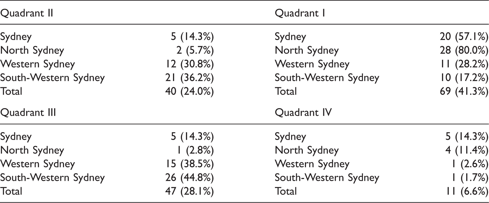
Using Stochastic Frontier Analysis, this article examines the efficiency and effectiveness of financial inputs and demographic data for educational outputs as measured by the Year 12 results for New South Wales secondary schools using a panel dataset from 2005 to 2010. Effective schools, in these analyses, are those that have higher Year 12 results than expected given their students’ prior performance and socio-economic status as well as financial inputs. Results indicate that prior learning achievement in Year 10 has a large, significant and positive impact on the current Year 12 results. Using a quadrant method, for each school, the efficiency score and the median Year 12 result are plotted separately for each of the three regions across New South Wales and a further quadrant plot is presented for the four Metropolitan districts in Sydney. Overall 37.5 per cent of schools are efficient and effective schools and 30 per cent are neither efficient nor effective.

Introduction

Over the last decade increasing attention is being paid to the performance accountability of Commonwealth and State government funds devoted to school education in Australia. In order to analyse the efficiency of schools, a dataset of public secondary schools in the Australian state of New South Wales (NSW) containing school financial and demographic data as well as Year 12 results is used in a Stochastic Frontier Model to produce efficiency scores. These scores are then analysed using a quadrant method. The key interest in this article is the identification of schools which are efficient and effective whereby schools that show higher results than expected given their students’ socio-economic background and prior achievement are considered to be effective ones.

In 2010, enrolment in public schools – also known as government or state schools – consists of about two-thirds of all children in Australia. State and Territory funding for public and private schools is $26.3 billion and $2.5 billion, respectively, and Federal funding is $2.1 billion and $5.5 billion, respectively. Considering the amount of money spent on public education there is only a limited number of studies available that examine how efficiently the resources are being used by public schools in Australia. The education funding arrangements by the Federal Government are also described in Chakraborty and Blackburn (2013).

This study is part of a series using a dataset from the NSW Department of Education’s annual financial statements for primary and secondary schools in NSW which have investigated the efficiency of government schools from different aspects (Blackburn, Brennan, & Ruggiero, 2014; Chakraborty & Blackburn, 2013; Pugh, Mangan, Blackburn, & Radicic, 2015).

Chakraborty and Blackburn (2013) investigate the cost efficiency of primary and secondary schools using the operating expenditure per student as the output with the Australia’s National Assessment Program – Literacy and Numeracy (NAPLAN) results for Grades 3 and 5 as some of the inputs. ‘The study found that social disadvantage in primary schools exerts a strong negative impact on students’ achievement scores causing inefficient use of available resources’ (p. 127).

Pugh et al. (2015) estimate the effects of school expenditure on school performance (the Australian Tertiary Admission Rank (ATAR) score), using a dynamic panel analysis from 2006 to 2010. Using a quadratic function for size of school, the results indicate that the size impact increases the estimated effects on the median ATAR score until the size of the school reaches approximately 1,500 students. In schools with more than 1,500 students the positive size impact decreases. The resource used in this article is ‘Increasing real aggregate expenditure per full-time equivalent’. The study finds that while an increase in expenditure does increase the estimated median ATAR score, the impact is small. The authors further recommend using a panel dataset and dynamics.

As a result of the Gonski’s Review (2011) which includes recommendations for a new national school funding model, measuring the overall performance of each school and reporting the technical efficiency index for public school funding policies has increased in importance. The ‘Schools Issues Paper’ (Commonwealth of Australia, 2014) also stresses the importance of a ‘greater focus on the equity, efficiency and effectiveness of school service delivery’ in relation to school funding. These issues are the focus of the empirical modelling in this article.

To our knowledge, no earlier study examines the effects of prior attainment in Year 10 (the median value of the School Certificate) on Year 12 outcomes in the context of Australian secondary schools. Nor are we aware of any study that has divided the total expenditure of schools into average teachers’ salaries and average salaries of other staff. However, using Stochastic Frontier Analysis (SFA) modelling, we expect to confirm the findings of earlier studies which show that prior achievement (i.e. Year 10 results in this study) is a strong indicator of future success.

As no socio-economic status (SES) variable is available in the current dataset, a number of variables are used as proxies. We use dummy variables for region, ratio of female students, the proportion of Indigenous Students, the proportion of students attending school and the apparent average retention rate. Further, using a graphic quadrant analysis, it is possible to identify schools that are efficient and effective by each of the three regions in NSW. The Metropolitan region of Sydney is further subdivided into four regions. This quadrant analysis indicates very clearly the large percentage of schools (61.7 per cent) that have an above average efficiency score while 46.3 per cent of schools have an above average ATAR score.

The major objectives of our study are: (1) to identify the secondary schools that are efficient in managing their resources while delivering the required educational outcomes; and (2) to identify the factors that account for the differences in the median ATAR between schools, in particular the role of prior academic achievement, disaggregated school financial resources and dynamic effects. The specific policy context of this study are current reforms involving a movement away from a centrally determined school spending regime towards a decentralised model of school level spending and staff hiring.

The NSW secondary school system

To put the dataset used in the analyses reported in this article in context, we provide an overview of the funding and enrolment systems operating in public schools in NSW. In this study, we are only concerned with government schools which are centrally funded. The level of funding for schools for education and training is determined by the NSW State Budget process. Approximately 82.5% of school recurrent resources are issued through NSW state allocations, another 13 per cent are allocated by Commonwealth Government allocations and school derived revenue makes up approximately five per cent.

Staff positions constitute about 81% of the operational costs of a school. The number of students in Years 7–10 and 11–12 determine the number of teachers in the general teacher category. Low SES schools also receive funding under the Priority School Funding Scheme whilst salaries of other staff and non-teaching staff are allocated on the basis of student enrolments. Additional funding is available for circumstances such as urgent minor maintenance, geographic isolation and socio-economic considerations. The number of students is used to calculate the additional entitlements where the most important factors are disability and SES dimensions.

A key objective in the NSW secondary school system is a focus on maximising student year 12 results which are used to determine eligibility for university entry. The Year 10 results are an important prior determinant of achievement in upper secondary schooling.

Students wishing to enrol in a public school in NSW are usually required to enrol in the primary school or high school in their local designated enrolment area. Further to this, schools are expected to accept all students for enrolment residing in the school’s designated enrolment area.

Background

The studies that have been reviewed for this article have been grouped into two sections. The first section focuses on studies that have used regression techniques. The second section focuses on studies which have used two types of efficiency analysis, namely Data Envelopment Analysis (DEA) and SFA.

Prior research using regression techniques

Todd and Wolpin (2003) consider methods for modelling a production frontier. Much of the discussion is on data at the student level. However, the authors recognise that both school and family inputs, current and past, are important. Data are usually gathered at the school which implies school data are readily available but not necessarily family data. Fredriksson, Öckert, and Oosterbeek (2013) use data from Swedish one-school districts to evaluate the long-term effects of class size. They conclude that ‘smaller classes in the last three years of primary school (age 10 to 13) are beneficial for cognitive and non-cognitive ability at age 13, and improve achievement at age 16’ (p. 249). They also find that larger class sizes decrease the earnings of students later in their adult lives.

Goldhaber and Brewer (1997) use the first two waves of the US National Education Longitudinal Study of 1988 (NELS). Information about 8th and 10th grade marks as well as demographic information are used. Outcomes are usually standardized test scores which are regressed on a set of factors involving school inputs and demographic data of the family. There is little agreement in this study as to the most important factors.

Hanushek, Rivkin, and Taylor (1996) use student data from the US High School and Beyond (HSB) Panel Data Survey from 1980, 1982, 1984 and 1986. There are two attainment variables – composite 12th grade test scores and years of schooling attained. The authors use a two-stage regression framework to analyse the impact of aggregation. The results show that using aggregated data overestimates the influence of school expenditure on student characteristics.

Gyimah-Brempong and Gyapong (1991) use canonical regression models for graduating 12th grade students in Michigan, US at the district level in 1986/1987. They find that socio-economic characteristics (SEC) have positive and significant impacts on the output of education. There is a high correlation between SEC and school resources. The authors note that parents’ education is an adequate variable to use as a proxy for SEC. Past student achievements are also an important determinant of students’ performance.

Sellin (1990) investigates the effects of aggregation at the student level and class level. He explores whether ‘the influences of group related variables should be examined using students, classes or schools’ (p. 257). He suggests that it is possible that some variables will seem to have a much stronger effect at the school level. Sellin also notes that it is common practice to use class or school levels instead of a student level. He states that, resulting from aggregating the data, there is a loss of information which leads to differences between the regression results. Using ordinary least squares modelling, Cramer (1964) finds that unbiased estimates of the same parameter occur whether using individual observations or weighted group data.

These five articles illustrate the need to have less aggregated data and include all relevant variables especially prior achievement and SES factors. However this is not possible with the NSW dataset as school and student data are not collected. Further, including the financial detail requires all data to be aggregated to the school level. The article by Cramer (1964) indicates that the problems with grouped data may cause too many problems. Cramer also notes that the two estimates are generally highly correlated.

Previous Australian studies investigate the relationship between school performance and effectiveness and concentrate on the impact of the SES of students and their academic achievements. Drawing on Australian data from PISA, McConney and Perry (2010) used SES data to measure how student achievement in mathematics and science varies by school SES groups (quintiles). The authors find: (1) as the SES of each school group increases, the mean individual student achievement consistently increases, (2) students in the lowest school group quintile have consistent increases in student academic achievement as the SES for the individual student group increases, and (3) in Australia, the location of the school makes a significant difference to the mean achievement in mathematics and science.

Yates (2002) investigates the direction and magnitude of relationships between students’ optimism, pessimism and achievement in mathematics over time and considers ‘the influence of students’ Grade level and gender on these relationships’. The study uses a sample of students in Grades 3 to 7 in two government primary schools in South Australia three years apart. Correlations and regression models are used. Pessimism is associated with lower achievement both at the first stage of the study and in the second stage. Achievement in mathematics is most strongly connected to prior achievement and grade level.

Marks (2009) uses Australian data for students who participated in the 2003 PISA study to examine school sector differences. Regression analysis is used to estimate the models with variables representing school sector, socio-economic background and achievement (PISA score) with tertiary performance as the dependent variable. He concludes that moderate value-added effects for the school sector exist when prior achievement is considered.

Miller and Voon (2011) examine NAPLAN results for Australian schools from all states and territories and for three sectors of schools – government, catholic and independent – using regression models. The authors use data from 2008 and 2009. Test score data for 3rd, 5th, 7th and 9th graders are regressed against SES characteristics, type of school, percentage of female students, student attendance, school size, state and region. No information on prior academic achievement or school financial resources is used in their analysis. The estimated coefficients for the different NAPLAN tests and for different years are broadly the same. The school Index of Community Socio Educational Advantage (ICSEA) is the most influential variable. The Year 3 results show large differences across states and school types.

Adams (2012) uses NAPLAN data to explore trends in the reading and numeracy achievement of Australian students. Data from 2008 to 2011 are analysed for Years 3, 5, 7 and 9 in all Australian states and territories. Two models are estimated using ‘differences as outcome models that estimated group differences in gains and prediction models that predict a second performance using both an initial performance and background characteristics’ (p. 32). In both models, there is very little variation between gains. In areas with higher mean outcomes in terms of student performance, a tendency for less variation between schools and student subgroups exists.

Hill and Rowe (1998) use a multivariate multilevel to explain the variation in primary school students’ progress in their literacy achievement. Three waves of data (1992, 1993 and 1994) on literacy progress of primary school students in Victoria are used. Independent variables consist of prior achievement and social background including critical events. Students with a disability have a significant negative effect on literacy progress with prior achievement having a significant and positive effect.

Drawing on data for Spain from the PISA study, Perelman and Santin (2011) note that the aggregation of data to a school or district level imposes some limitation on disentangling the background of individual students. They use a parametric output distance function at the student level, controlling for potential endogeneity of school choice. Observed differences can be associated with the effort and motivation put in by teachers, parents and students. When the differences in school inputs, students’ background and other characteristics are taken into consideration in the model, the observed differences between the public and private-voucher schools vanish.

Keeves, Hungi, and Darmawan (2013) study the effects of SES, size and ability grouping of classes on science achievement of secondary school students in Canberra in the Australian Capital Territory. Using the three levels of student, classroom and school, the authors use a multilevel analysis controlling for student level effects. At the student level, father’s occupation, expected education, liking science and prior achievement directly influence science achievement. At the class level, prior achievement and class size positively affect science achievement.

Marks (2014) uses a panel dataset, NAPLAN, of students in Victorian government schools in Australia comprising students in Years 3 in 2008, Year 5 in 2010 and Year 7 in 2012 in order to investigate changes over time. Using a fixed effects model, Marks finds that prior achievement has a dominant influence even after differences in school and socio-economic backgrounds have been included in the model.

Van Ewijk and Sleegers (2010) use a meta-regression analysis of 30 studies on the effects on students’ test scores of their peers’ SES. These 30 studies produce large differences in their results. There are three sources of variation – measurement of the SES variable, sample characteristics and model specification. Dealing with endogeneity and omitted variable bias has many different outcomes. The different ways of estimating the SES variable can also influence the effect size. The effect does not differ between science, mathematics, language or country. Studies controlling for omitted variable bias find lower effects but the differences are not statistically significant. The results also suggest that not including prior achievement as a covariate can lead to upward bias in the effect estimates.

The studies which have been discussed in this first section cover Australian student assessment data and find both SES and prior attainment to be key explanatory determinants with prior achievement being the dominant influence.

Prior efficiency research using DEA

Mante and O’Brien (2002) assess the technical efficiency of 27 Victorian secondary schools using the DEA model and 1996 data and find many schools could increase their output by using their resources more efficiently. The authors state that, when adjustments for socio-economic disadvantages are made, the schools previously thought to be inefficient are not significantly less efficient than other schools.

Bradley, Draca, and Green (2004) use three different data sources to build a database of primary school students in the public education system in the Australian state of Queensland. They use the DEA model to investigate how socio-economic structure, demographic variables and the average prior ability of students impact on the school’s output measure which consists of average scaled literacy and numeracy for year 7. Their results indicate that the size of the school and the income variable have a positive impact while the proportion of Indigenous students is negatively related to the school’s efficiency.

Alexander, Haug, and Jaforullah (2010) use a two-stage (DEA and regression) analysis of the efficiency of secondary schools in New Zealand. They find that single-sex schools show higher achievement than co-educational schools and that main urban schools show higher achievement than rural and minor urban areas. In addition, results show that socio-economic deprivation is related to lower achievement whereas greater teacher experience and qualification levels are linked to higher achievement.

Blackburn et al. (2014) used a DEA model from 2010. Including an index for the socio-economic environment, their results suggest that efficiency gains are increased as the environment becomes more favourable.

In summary, these earlier studies show that variables, SES and prior achievement, are consistently estimated in the models. Other variables that are found to be significantly related to higher performance and achievement are the size of the school, teachers’ experience and qualifications, and school expenditure.

Prior efficiency research using SFA

Frontier methods are first introduced by Aigner, Knox Lovell, and Schmidt (1977) and Meeusen and van den Broeck (1977) independently. Jondrow, Knox Lovell, and Schmidt (1982) propose a method of separating the error term of the SFA model into two components for each observation. Pitt and Lee (1981) use production function models with cross-section data over time. They assume that time invariant efficiency is tenable over a long-panel dataset. The time invariant assumption is relaxed in Battese and Coelli (BC) (1992). Battese and Coelli (1995) and others extend the estimation to a single-stage approach.

In a study of Portuguese schools, Pereira and Moreira (2007) use a panel dataset at the school level for 555 schools in 2003/2004 and 545 schools in 2004/2005. The SFA model was used with a log-linear specification. Results are ‘less sensitive to the presence of outliers and allowed the possibility of making inference about the contribution of inputs’ (p. 3).

Using data from 283 school districts in Kansas, US and a three-year panel dataset (2002–2005), Chakraborty (2009) estimates two SFA models using the BC models. The test score data are aggregated to the district level as many of the input variables are only available at the district level. The authors note that Kansas schools are generally efficient, however SES factors have a significant impact on achievement scores.

Kirjavainen (2012) estimates different SFA models to calculate the efficiency of Finnish general upper secondary schools using a school-level panel dataset from 2000 to 2004. There are 436 schools, but the panel is unbalanced. The output is the grade in an examination while the main inputs consist of the school grade point average, parental background, school resources and the length of studies. The efficiencies and the rankings of schools vary between models. These models allow the separation of random and fixed effects from inefficiency. Hence, they allow for heterogeneity and omitted variable bias.

The articles using the SFA model used a panel dataset and found SES and students’ prior achievement and family background were the strongest predictors of performance.

Comparison of DEA and SFA models

Bifulco and Bretschneider (2003) note that, if the variables have significant measurement errors, then, if the estimation methods require exogenous inputs, the inaccuracy can be substantial. The SFA model incorporates an efficiency term and a random error as part of the estimation of the model. Most researchers use a half-normal distribution for the efficiency term. Specifying a half-normal distribution generates more reliable estimates of the technical efficiency.

Grosskopf, Hayes, and Taylor (2014a) focus on modelling and measurement choices to analyse efficiency in education. The authors note their agreement with economists that the value-added measure is the best way to estimate student performance. However to calculate the value-added measure, the data need to be panel data at the student level and not aggregated upwards. The authors note that models with multiple inputs and outputs need a DEA model whereas models with a single output can use a SFA model. Most of the educational models have only one input so the SFA may be the most appropriate model.

Mizala, Romaguera, and Farren (2002) use the SFA and the DEA methods for measuring efficiency. The two models give a similar ranking of primary schools in terms of efficiency. The data consist of a random sample of 2,000 Chilean schools classified by type of school and include a socio-economic index and a vulnerability index for measuring the performance and efficiency of schools using the academic performance of primary school students. An efficiency-achievement matrix, using four quadrants to identify the schools which are inefficient and ineffective as well as other combinations of efficiency and effectiveness, is also created.

Grosskopf, Hayes, and Taylor (2014b) use a dataset from primary and secondary schools in Texas, US as an empirical example of assessing efficiencies in school performance. Measuring production efficiency can be calculated by maximising the output for a given set of inputs or a given budget. The authors estimate three models – SFA, DEA and Corrected Ordinary Least Squares (C-OLS). The authors note the different assumptions that the DEA and SFA models use. The DEA model assumes all variables are measured without error. It seems very unlikely that the education variables are measured without error. The SFA model allows different assumptions made about the error term. Grosskopf summarises her results by stating that ‘applying techniques to data are sensitive to the modelling choices’ (p. 202).

These studies show that the variables, SES and prior achievement, are very important in almost all the models. Using the DEA model has underlying assumptions that may not apply to educational data.

In earlier articles, the SFA model is not used in measuring the efficiency of Australian secondary level government schools using Year 10 public exam results as well as final year 12 public exam results which are used to determine students’ university entrance scores (ATARs). We consider the SFA approach as novel for Australian data which will add to the existing body of our knowledge about school efficiency and effectiveness. Further, both at the state regional level and at the sub-region in metropolitan areas, using efficiency matrices and graphs provide an illustration of the schools that are efficient and effective.

Data and descriptive statistics

The analysis presented in this article use a panel dataset from the Department of Education’s annual financial statements. These statements contain information on several inputs/outputs and other socio-economic variables for all public secondary schools in NSW for the years 2005–2010. The final dataset includes information on 339 secondary schools that are split into three regions – Metropolitan, Hunter and Illawarra, and Country – to enable the exploration of regional differences throughout NSW. While NSW has additional regions, their school numbers are small and thus are considered as one group – Country.

Most of the schools (49%) are in the Metropolitan region with 22 per cent in the Hunter and Illawarra region and 29 per cent in the Country. The Metropolitan region encompasses the city of Sydney which for the purpose of these analyses is divided into four districts, namely Sydney, North Sydney, Western Sydney and South-Western Sydney to explore the efficiency scores relative to the ATAR results for each school. The Hunter and Illawarra region is to the north and south, respectively, of the Sydney region. Schools outside the Greater Metropolitan Area are considered to be part of the Country region.

In NSW, the aggregated scores in the Higher School Certificate examinations at the end of Year 12 are used by parents, students and policy makers to rank the performance of schools. The ATAR is used as the main criteria for entry into university. It is a percentile score which denotes a student’s ranking relative to their peers in the Higher School Certificate. For example, an ATAR score of 99.0 means that the student is better than 99% of his or her peers, and ranks lower than 0.95% of peers (as the maximum score is 99.95).

In the context of this study, one potential problem is using the ATAR as an output variable. We assume that the distribution of the median ATAR is consistent over the six year period. Note that the questions on the examination articles vary from year to year and also the composition of students and their abilities. The average ATAR increases 6.1% from 2005 to 2009. There is very little difference in the kernel densities of the scores for 2005 to 2007. However, when the kernel density for the years from 2007 to 2010 are estimated, the kernel density functions for the ATAR for 2009 and 2010 shift to the right of 2007 (Figure 1). The shift is very small, indicating that the measurement of the median ATAR should not pose a problem as it indicates consistency of the measure over the period 2005 to 2010. The kernel densities justify the assumption of consistency.

Figure 1.

Kernel Density Functions for ATAR for the Years 2007 to 2010.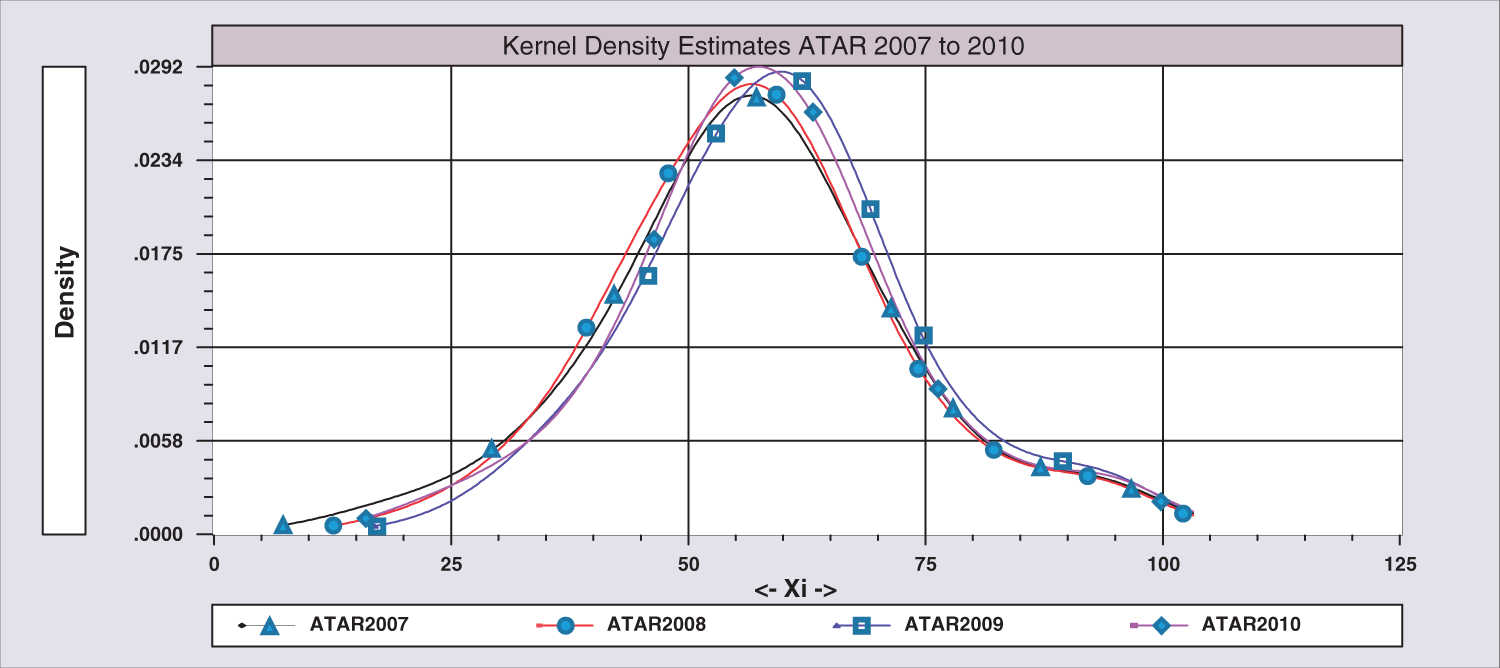

In this study, we use NSW Year 10 School Certificate Examination Results from 2005 to 2010. In Year 10, all students sit an external examination in English, Mathematics, Science, History and Geography. These examinations are moderated and marked externally. The median School Certificate result for each school is an indication of the prior learning/achievement of students at each school. This is the only state-wide measure available to indicate the ability of a student in a particular school. The correlation between the ATAR and School Certificate median for each school and year is 0.88.

The school and non-school inputs used in this study are measured as student–teacher ratio, average contract salary for teachers and support staff, and the average years of service of teachers which give an indication of teacher experience in the school (Table 1). School Own Source Expenditure from funds raised in the school is identified as a separate expense item. The three expenditure variables are deflated using the CPI for Sydney with a base year of 2005 giving real expenditure. Further, the variables are on a per capita basis to control for the variation in the size of the schools.

Table 1.

Definitions of the variables in the dataset.

Variable	Definition
ATAR	Median ATAR for each school
Hunter & Illawarra	Dummy variable = 1 if schools is in the Hunter and Illawarra area
Country	Dummy variable = 1 if schools is outside the greater metropolitan area
No. of students	Number of students in the school
Teachers’ salaries per student	Average salaries for teachers per student $
Other staff salaries per student	Average salaries of other staff per student $
Female ratio	Ratio of female students in the school
Yrs of service	Average years of service of teachers
Student teacher ratio	Ratio of students to teachers
School own expenditure	School own source expenditure per student
Median School Cert.	Median mark for the school certificate
Indigenous students per student	Proportion of indigenous students per student
Retention	Apparent average retention rates
Attend	Proportion of students attending school

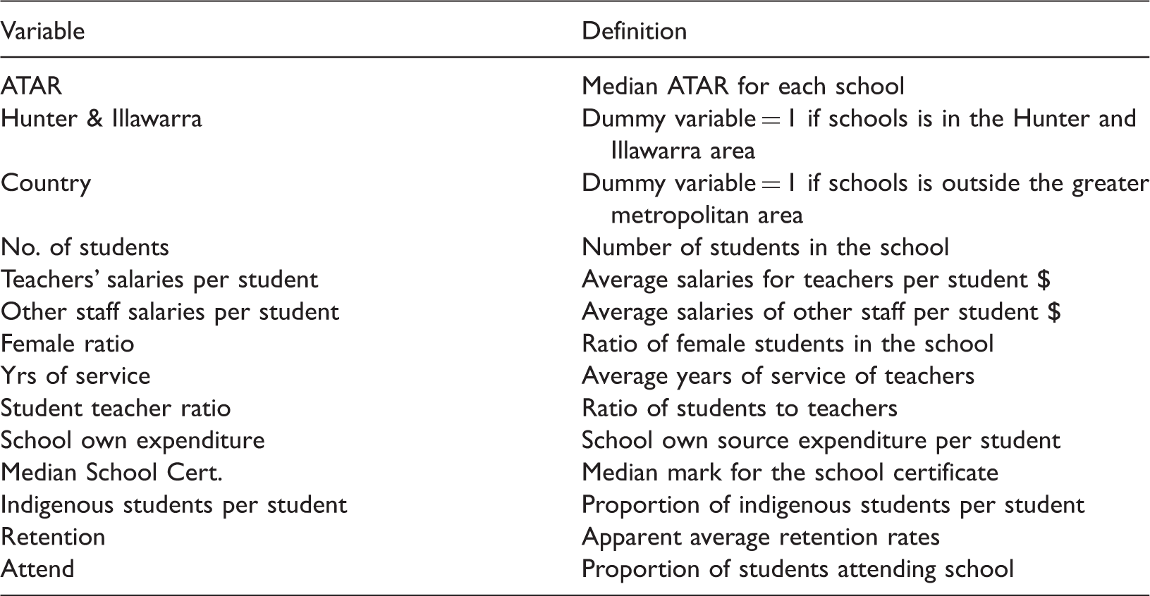
The variables used to control for the school environment are the ratio of female students in the school and the proportion of Indigenous Students per student in the school. Other characteristics of schooling such as apparent retention rates and student attendance are also used. Apparent retention measures the extent to which students in NSW public schools progress to their final year of schooling. The term ‘apparent’ is used because the measurement is based on the total number of students in each year level compared to the number in an earlier year, rather than by tracking the retention of individual students. Only full-time students are counted in the calculation of apparent retention.

The Family, Occupation and Education Index (FOEI) is the socio-economic index variable used in NSW. At the time of writing this article, the authors were only able to access FOEI data for years 2009 and 2010. As more years of FOEI data become available, it will be included in future models. Pugh et al. (2015) have included this variable in their model but it is unclear how the missing observations are treated.

The descriptive statistics for the dataset being used are shown in Tables 1 to 3. Table 1 details the definition of the different variables. Tables 2 and 3 present the descriptive statistics for each variable averaged over the six years for all schools and for each of the three regions. The number of students in a school varies from 145 to 2,029. The range for the median ATAR in the schools ranges from 11.5 to 99.35. The range for average teachers’ and other staff salaries per student are large considering that these are per student values.

Table 2.

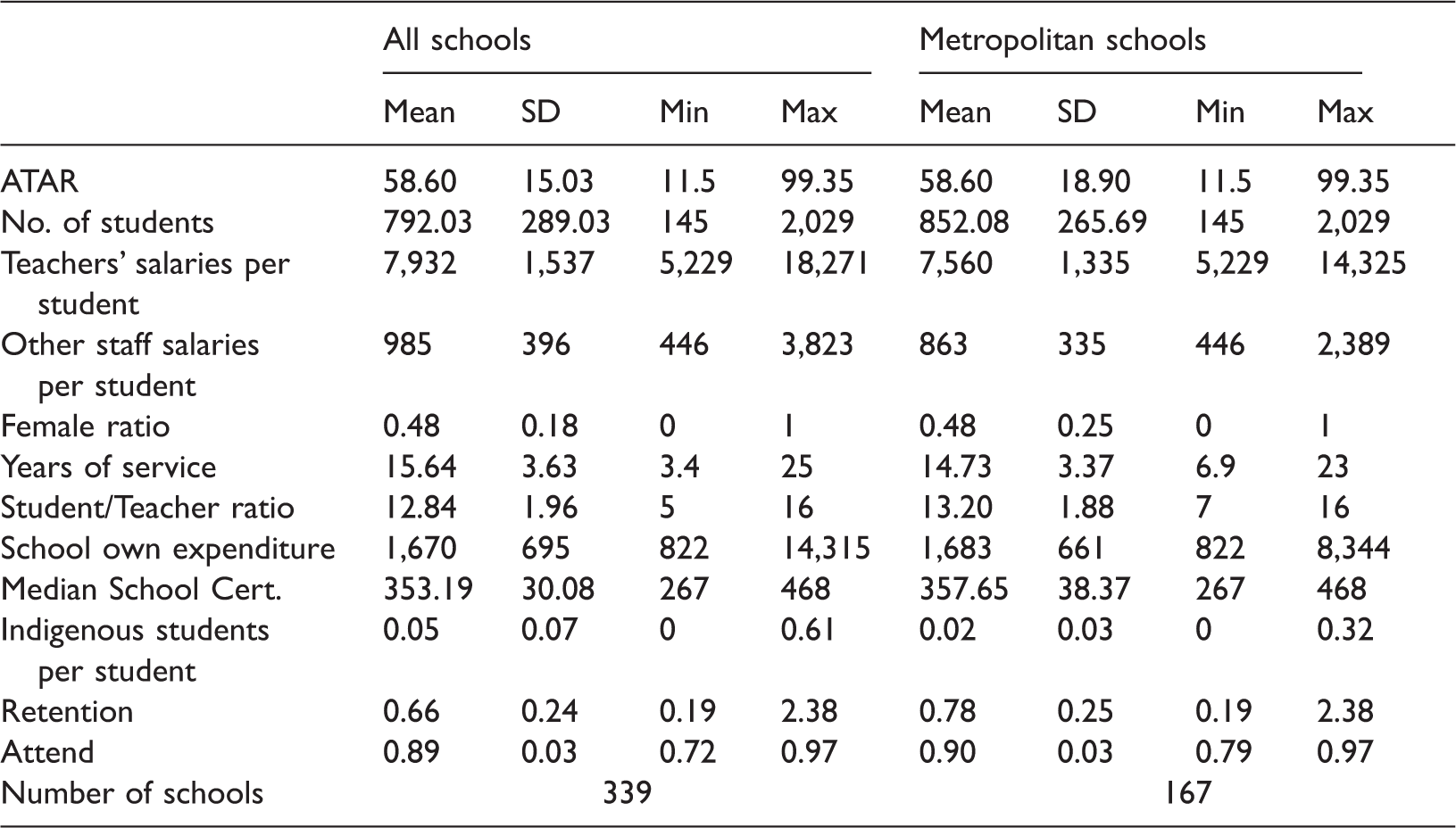
Descriptive statistics for all schools and metropolitan schools for 2005–2010.

	All schools				Metropolitan schools
	Mean	SD	Min	Max	Mean	SD	Min	Max
ATAR	58.60	15.03	11.5	99.35	58.60	18.90	11.5	99.35
No. of students	792.03	289.03	145	2,029	852.08	265.69	145	2,029
Teachers’ salaries per student	7,932	1,537	5,229	18,271	7,560	1,335	5,229	14,325
Other staff salaries per student	985	396	446	3,823	863	335	446	2,389
Female ratio	0.48	0.18	0	1	0.48	0.25	0	1
Years of service	15.64	3.63	3.4	25	14.73	3.37	6.9	23
Student/Teacher ratio	12.84	1.96	5	16	13.20	1.88	7	16
School own expenditure	1,670	695	822	14,315	1,683	661	822	8,344
Median School Cert.	353.19	30.08	267	468	357.65	38.37	267	468
Indigenous students per student	0.05	0.07	0	0.61	0.02	0.03	0	0.32
Retention	0.66	0.24	0.19	2.38	0.78	0.25	0.19	2.38
Attend	0.89	0.03	0.72	0.97	0.90	0.03	0.79	0.97
Number of schools	339				167

Table 3.

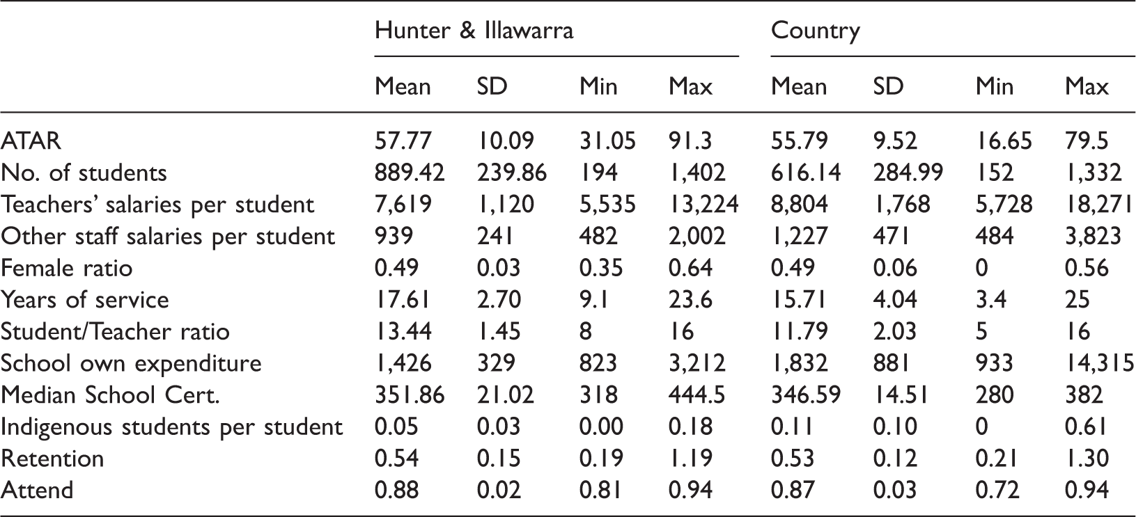
Descriptive statistics for Hunter & Illawarra schools and country schools for 2005–2010.

	Hunter & Illawarra				Country
	Mean	SD	Min	Max	Mean	SD	Min	Max
ATAR	57.77	10.09	31.05	91.3	55.79	9.52	16.65	79.5
No. of students	889.42	239.86	194	1,402	616.14	284.99	152	1,332
Teachers’ salaries per student	7,619	1,120	5,535	13,224	8,804	1,768	5,728	18,271
Other staff salaries per student	939	241	482	2,002	1,227	471	484	3,823
Female ratio	0.49	0.03	0.35	0.64	0.49	0.06	0	0.56
Years of service	17.61	2.70	9.1	23.6	15.71	4.04	3.4	25
Student/Teacher ratio	13.44	1.45	8	16	11.79	2.03	5	16
School own expenditure	1,426	329	823	3,212	1,832	881	933	14,315
Median School Cert.	351.86	21.02	318	444.5	346.59	14.51	280	382
Indigenous students per student	0.05	0.03	0.00	0.18	0.11	0.10	0	0.61
Retention	0.54	0.15	0.19	1.19	0.53	0.12	0.21	1.30
Attend	0.88	0.02	0.81	0.94	0.87	0.03	0.72	0.94

We consider the possible effect that the proportion of Indigenous students in the school per student might have on the average Teachers’ and other staff salaries per student. It is expected that more resources may be granted for schools with a higher proportion of Indigenous students. As the average proportion of Indigenous students increases, the average salary of other staff shows a small increase.

In Figure 2(a) to (c), all three regions show a definite downward trend in the average salaries of teachers and other staff as the number of students in the school increased. There are a few outliers in each region. As the average size of the school increases, the average salaries for teachers per student decreases from approximately $12,000 to $6,000 for all three regions. Apart from two outliers, the average school expenditure per student for the Country region decreases from approximately $3,000 to about $1,000 when the average number of students increases. The decrease is not as evident in the other two regions.

Figure 2.

(a) Average teacher salaries, other staff salaries and school expenditure per student for Metropolitan Schools. (b) Average teacher salaries, other staff salaries and school expenditure per student for Hunter and Illawarra Schools. (c) Average teacher salaries, other staff salaries and school expenditure per student for Country Schools.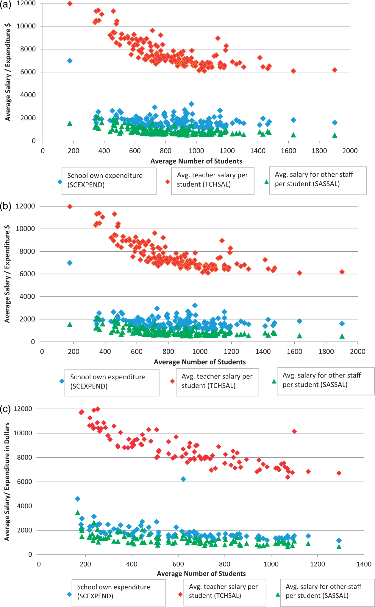

Technical efficiency and Production Frontier Models

Concept of efficiency

There are two types of efficiency – economic efficiency, which involves resource allocation and technical efficiency, which involves decisions made at the school level to maximize output given a certain level of inputs. Schools in NSW have no jurisdiction over how the resources are allocated to the school. Therefore, this article considers technical efficiency to be the most relevant measure for these schools. Using technical efficiency, it is possible to determine whether increasing outputs can be achieved by managing inputs more efficiently.

There are two models that can be used to calculate the technical efficiency for each school – the SFA model and the DEA. In this article we only use the SFA model as the DEA models have some assumptions that are not relevant in this project. The DEA model assumes all variables are measured without error which is unlikely in the education context. The SFA model allows different assumptions made about the error term.

Stochastic Frontier Production model

SFA models use the concept of an economic production function which estimates the maximum output reached given a set of inputs. There are some important empirical difficulties with applying the methodology of economics to the education field. Pereira and Moreira (2007) note that the first problem is the definition of output while the second relates to the factors beyond school inputs. The first problem is easily addressed in our analyses as the output in our study is clearly defined as the HSC examination which is undertaken by most students in year 12 in NSW. However, their second concern is more problematic as it relates to demographic factors of students, interactions with colleagues and ability. They note that some of the problems can be lessened by using data either at the individual student level or aggregated to the school level. Our data are aggregated to the school level.

Time-invariant technical efficiency

There are two models for estimating efficiencies that we consider in this article – the time-invariant technical efficiency and time-varying technical efficiency.

For the panel data model, we have observations on n schools over t time periods. Note the error term of the stochastic frontier production function has two components which enables statistical noise and technical inefficiency to be separated. Thus u_i is a non-negative term to account for technical inefficiency while $v_{\mathrm{it}}$ is a symmetric error term to account for other random effects. Here u_i is the amount by which the observed individual school fails to reach the optimum output. The model is

$$y_{\mathrm{it}}=\beta \text{'}{x}_{\mathrm{it}}+v_{\mathrm{it}}-u_{i}i=1,\dots n,t=1,\dots T$$

(1)

where $y_{\mathrm{it}}$ is the output (for school i in time t) and $x_{\mathrm{it}}$ is a vector of inputs in each period, β is the parameter to be estimated, $v_{\mathrm{it}}$ is the idiosyncratic error term for each period with $v_{\mathrm{it}}\hspace{1em}\sim N(0,{\sigma }_v^2)$ and $u_i=u_{\mathrm{it}}$ are the efficiencies for each school in each period with $u_{\mathrm{it}}\hspace{1em}\sim \mathrm{iid}{N}^{+}(0,{\sigma }_u^2)$ . As we assume that $u_{\mathrm{it}}$ are time invariant effects, it follows that $u_i=u_{\mathrm{it}}$ . Here the structure of technical inefficiency does not allow for change over time as it remains constant over time. The efficient term is estimated as

$$E(u_{\mathrm{it}}|e_{\mathrm{it}})=\frac{\sigma \lambda }{(1+{\lambda }^2)}\{\frac{\phi (z_{\mathrm{it}})}{(1-\Phi (z_{\mathrm{it}})}-z_{\mathrm{it}}\}$$

(2)

where $\sigma =({\sigma }_v^2+{\sigma }_u^2{)}^{/12}$ , $\lambda ={\sigma }_u/{\sigma }_u{\sigma }_v{\sigma }_v$ and $z_{\mathrm{it}}=\frac{e_{\mathrm{it}}\lambda }{\sigma }$ . This is the time invariant inefficiency model by Pitt and Lee (1981). Here φ and Φ represent the density function and cumulative distribution of the standard normal, respectively.

Time-varying technical efficiency

Battese and Coelli (1992) consider a stochastic frontier production function using an exponential specification of time varying effects where the assumptions about $u_{\mathrm{it}}$ are modified. The model is

$$y_{\mathrm{it}}={\beta }_{\mathrm{ot}}+\sum _n{\beta }_{\mathrm{nit}}{x}_{\mathrm{nit}}+v_{\mathrm{it}}-u_{\mathrm{it}}={\beta }_{\mathrm{it}}+\sum _n{\beta }_{\mathrm{nit}}{x}_{\mathrm{nit}}+v_{\mathrm{it}}$$

(3)

where ${\beta }_{\mathrm{it}}={\beta }_{\mathrm{ot}}-u_{\mathrm{it}}$ . Here ${\beta }_{\mathrm{ot}}$ is the production frontier intercept common to all schools in the time period t and ${\beta }_{\mathrm{it}}$ is the intercept for school i in period t. Further $u_{\mathrm{it}}=\beta (t)u_i$ , $u_i\hspace{1em}\sim \mathrm{iid}{N}^{+}(0,{\sigma }_u^2)$ and $\beta (t)=\exp [-\eta (t-T)]$ . Note that $u_{\mathrm{it}}$ is a half-normal distribution, T is the number of periods in the balanced panel and η is an unknown scalar parameter. The function $\beta (t)$ satisfies the following property $\beta (t)\ge 0$ . Here $u_{\mathrm{it}}$ represents the non-negative school effects which increase at a decreasing rate, remain constant or decrease at an increasing rate if $\eta >0,\eta =0\mathrm{or}\eta <0$ , respectively (Battese and Coelli, 1992, p. 154). Note that, when $\eta =0$ , the BC model reverts to the Pitt/Lee (PL) model.

The model used is

$$\log (\mathrm{atar}{)}_{\mathrm{it}}={\beta }_0+{\beta }_1\mathrm{Hunter}\hspace{1em}\&\hspace{1em}{\mathrm{Illawarra}}_{\mathrm{it}}+{\beta }_2{\mathrm{Country}}_{\mathrm{it}}+{\beta }_3\log (\mathrm{teachers}\text{'}{\mathrm{salaries}}_{\mathrm{it}})+{\beta }_4\log ({\mathrm{otherstaffsalaries}}_{\mathrm{it}})+{\beta }_5{\mathrm{femaleratio}}_{\mathrm{it}}+{\beta }_6\log (\mathrm{yrs}\mathrm{of}{\mathrm{service}}_{\mathrm{it}})+{\beta }_7\log (\mathrm{student}\mathrm{teacher}{\mathrm{ratio}}_{\mathrm{it}})+{\beta }_8\log (\mathrm{school}\mathrm{own}{\mathrm{expend}}_{\mathrm{it}})+{\beta }_9\log (\mathrm{median}\mathrm{school}{\mathrm{cert}}_{\mathrm{it}})+{\beta }_{10}\mathrm{Indigenous}{\mathrm{students}}_{\mathrm{it}}+{\beta }_{11}{\mathrm{retention}}_{\mathrm{it}}+{\beta }_{12}{\mathrm{attend}}_{\mathrm{it}}+{\beta }_{13}{\mathrm{year}}_{\mathrm{it}}+v_{\mathrm{it}}-u_i$$

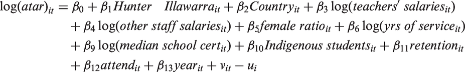
Stochastic Frontier Production model’s results

A number of SFA models are estimated and the results are presented in Table 4. Note that the error term in SFA models is allowed to vary. Some of the options are the time invariant models – the half-normal and the exponential distributions – and the time dependent distribution. The first model is a pooled model where panel effects are not considered. The second model is the time invariant PL model where the panel data are used and the distribution of the error term, u_i, is assumed to be a half-normal distribution. Further, as heteroscedasticity (HET) is expected in the model, a heteroscedastic model is estimated for the PL model. We assume that the two variables most likely to be the cause of heteroscedasticity are school expenditure and teachers’ salaries. The PL HET (PLH) model results are in column 3 of Table 4. The BC model is also estimated as this is a time varying model. This model has an error term, $u_{\mathrm{it}}=\exp [-\eta (t-T)]|u_i|$ , which is dependent on time with u_i being a half-normal distribution. Note that, when the data are very consistent with the model, the BC model produces satisfactory results. Accordingly, we report the BC model as one of the models in Table 4. Note that the estimated coefficients are very similar in each of the three SFA models.

Table 4.

Results from the SFA Models for the panel dataset from 2005 to 2010.

Dependent variable: Log(ATAR) for each school
	(1) Pooled	(2) Pitt/Lee	(3) Pitt/Lee Het	(4) Battese/Coelli
Constant	−3.003***	−2.751***	−2.541***	−2.669***
Hunter & Illawarra	0.028***	0.030***	0.022***	0.028***
Country	0.047***	0.055***	0.047***	0.050***
Log (teachers’ salaries per student)	−0.086	−0.080	−0.143***	−0.069
Log (other staff salaries per student)	−0.061***	−0.086***	−0.059***	−0.088***
Female ratio	0.036***	0.039***	0.032***	0.035***
Log (yrs of service)	0.073***	0.093***	0.113***	0.087***
Log (student/teacher ratio)	0.061	0.078	0.028	0.070
Log (school own expenditure)	0.094***	0.073***	0.062***	0.063***
Log (Median School Cert.)	1.750***	1.698***	1.729***	1.674***
Indigenous students per student	−0.035	−0.087*	−0.095**	−0.070
Retention	0.018**	0.031***	0.024***	0.030***
Attend	0.405***	0.307***	0.253***	0.324***
Year	0.003***	0.005***	0.004***
Lambda	2.753***	1.036***	6.346***	0.762***
Sigma (u)	0.100***	0.059***	0.054***	0.043***
Eta				0.127***
School own expenditure			−0.0006***
Teachers’ salaries			0.0006***

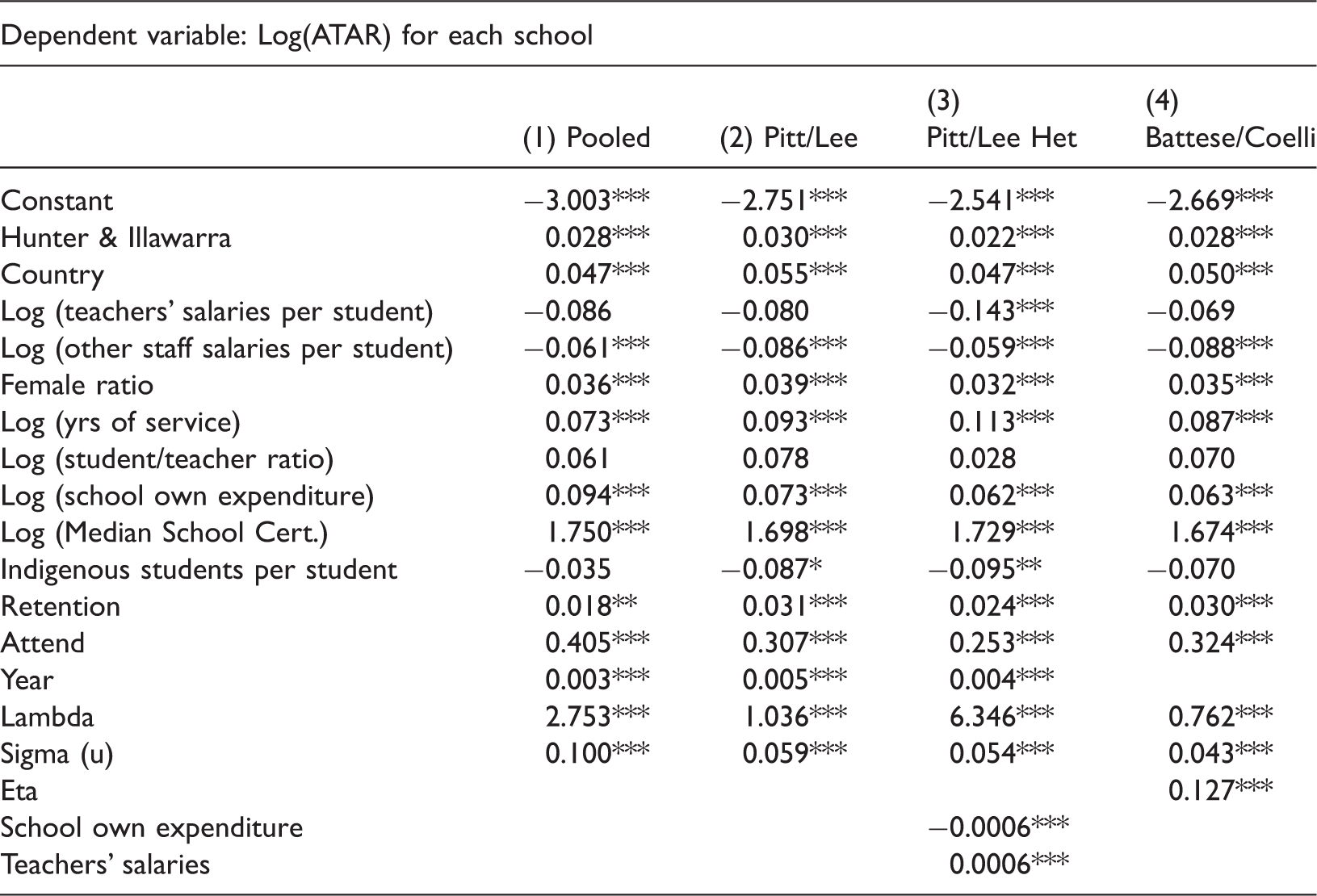
Note: ***, ** and *, denote significance at the 0.01, 0.05 and 0.10 levels, respectively.

The output from these models is the technical efficiency for each school. Using any one of the first three models, there is only one technical efficiency for all six years for each school. However, the BC model allows the efficiency to vary from year to year and thus a technical efficiency is generated for each of the six years for all schools. Kernel density functions are calculated for the four models. These functions show that there is very little difference between the PL model, the Pitt/Lee heteroscedasticity (PLH) model and the BC model. However there is a considerable difference between the pooled model and the PL model. There is evidence in the literature that different stochastic frontier models produce different outcomes. However with this set of data, we show that the decision to use various error terms has little impact on the estimated coefficients and also the technical efficiencies.

log(ATAR) is not a dependent variable. Should the variable, log(Median School Cert.) be lagged by two years? Our original dataset has data from 2005 to 2010, but the value of log(Median School Cert.) in 2005 actually applies to the students in 2007. Thus we estimate models using data from 2007 to 2010 – one with log(lagged Median School Cert.) values and the other without lagging this variable. A frontier model using exponential distribution assumptions gives results for both datasets and thus allows us to compare the results. The levels of significance are very similar for the variables in each model as are the estimated coefficients where the difference is less than 0.02 with two exceptions – the Attend (i.e. the proportion of students attending school) and the log (of the Median School Certificate) variables where the difference is 0.136 and 0.08, respectively. As a result, we have used all the data and not lagged the variable, log (of the Median School Cert.). A dynamic model is also estimated but the estimated coefficient of the lagged dependent variable is not significant.

As a check on the six year panel results (taking into account that FOEI is only available for 2 calendar years 2009 and 2010), we estimate the model for these two years with and without the FOEI variable. The results from this estimation indicate that including the FOEI variable in the equation does not indicate it to be very important, thereby indicating the much greater influence of the Year 10 School Certificate exam results (the prior attainment variable), on Year 12 ATAR scores.

In Table 4, the estimated coefficients are very similar between the three models – PL, PLH and the BC model. The level of significance is less than 1% for most of the variables. The signs of the significant coefficients are all as expected. As the variables, log(Teachers’ Salaries per Student) and log(Other Staff Salaries per Student), are negative, the most plausible reason is that economies of scale result in less State Government finance. The estimated coefficient for log(Median School Cert.) implies that if the School Certificate median result increases by 1%, the ATAR increases by 1.73% for the HET model. This is a large and elastic impact on the ATAR. No other variable has the same impact size. The Attend variable (the average yearly proportion of students attending school) is positive and significant with an estimated coefficient of 0.253 in the PLH model. Thus if Attend increases by 0.1, the ATAR increases by 2.53%. This is a large increase indicating the important of attendance.

The estimated coefficients for the Hunter and Illawarra and Country regions are positive and very significant. Moving from a metropolitan school to a country school, the average ATAR scores increase by 4.7%. Part of the explanation for this increase is the very large spread of ATAR scores and efficiency values for the Metropolitan schools.

The main interest in the results is the technical efficiencies that are produced. Note that the BC model is a time variant model and thus there is an efficiency score for each year for each school. This complicates the comparison between the PLH model and the BC model. However, the correlation coefficient for all the schools between the PLH efficiencies and the BC averaged efficiencies is 0.965. As a result, the PLH efficiencies are used in the rest of this article.

The efficiencies for the schools are further separated into three regions – Metropolitan, Hunter and Illawarra and Country. It is expected that the efficiencies will vary by region. Table 5 details the statistics for the three regions. The differences between the regions for the mean ATAR scores and the efficiencies are not significant. The maximum efficiencies are very similar but the Hunter and Illawarra region has the highest minimum ATAR score (43.17) as well as the highest average efficiency score (0.9635).

Table 5.

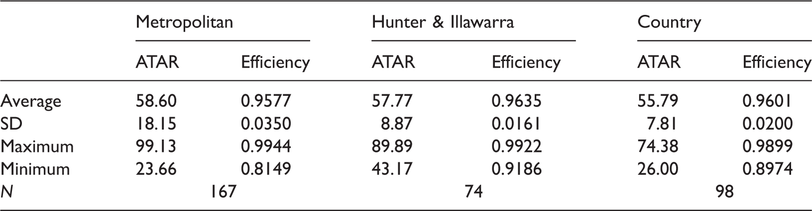
Descriptive statistics for the ATAR and efficiency for the three regions.

	Metropolitan		Hunter & Illawarra		Country
	ATAR	Efficiency	ATAR	Efficiency	ATAR	Efficiency
Average	58.60	0.9577	57.77	0.9635	55.79	0.9601
SD	18.15	0.0350	8.87	0.0161	7.81	0.0200
Maximum	99.13	0.9944	89.89	0.9922	74.38	0.9899
Minimum	23.66	0.8149	43.17	0.9186	26.00	0.8974
N	167		74		98

Mizala et al. (2002) introduce the concept of an efficiency-achievement matrix using four quadrants. Using the totals in Table 6, Quadrant I has 127 schools (37.5%) which indicates that these schools have an above average achievement (ATAR score) (effective) and an above average technical efficiency (efficient) implying that the schools achieve more output with fewer resources. Quadrant II has 82 schools that are efficient but achieve at a lower level. Quadrant III is the opposite of Quadrant I in that the 100 schools (30%) are inefficient and ineffective. Quadrant IV has 30 schools which are effective but not efficient. For the whole state, the average efficiency is 0.960 and the average ATAR is 57.6. Note that the percentage of schools in the Metropolitan region is 49.3%, in the Hunter and Illawarra region 21.8% and in the Country region 28.9%. Note that all schools are at least 80% efficient.

Table 6.

Efficiency-achievement matrix for the three regions in the state of New South Wales using the Pitt/Lee HET model.

Quadrant II		Quadrant I
Metropolitan	40 (24.0%)	Metropolitan	68 (40.7%)
Hunter & Illawarra	23 (31.1%)	Hunter & Illawarra	24 (32.4%)
Country	19 (19.4%)	Country	35 (35.7%)
Total	82 (24.2%)	Total	127 (37.5%)
Quadrant III		Quadrant IV
Metropolitan	47 (28.1%)	Metropolitan	12 (7.2%)
Hunter & Illawarra	19 (25.7%)	Hunter & Illawarra	8 (10.8%)
Country	34 (34.7%)	Country	10 (10.2%)
Total	100 (29.5%)	Total	30 (8.8%)

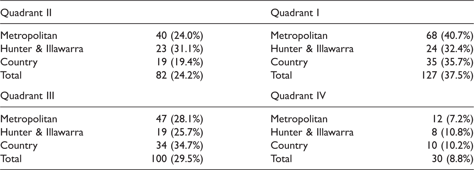
Figure 3(a) to (c) demonstrates these variations. It is obvious that the three regions have many schools with an excellent level of efficiency. For example, approximately 65 per cent of the Metropolitan schools are above the mean level of efficiency. In each of the regions, approximately 10 per cent or less have a high median ATAR and are inefficient. They also have 28.1% of schools in Quadrant III with low ATARs and low efficiency. The pattern for the Country schools is interesting as they are clustered around the average ATAR score and the average efficiency.

Figure 3.

(a) Efficiencies for the Pitt/Lee HET Model for the Metropolitan Region. (b) Efficiencies for the Pitt/Lee HET Model for the Illawarra and Hunter Region. (c) Efficiencies for the Pitt/Lee HET Model for the Country Region.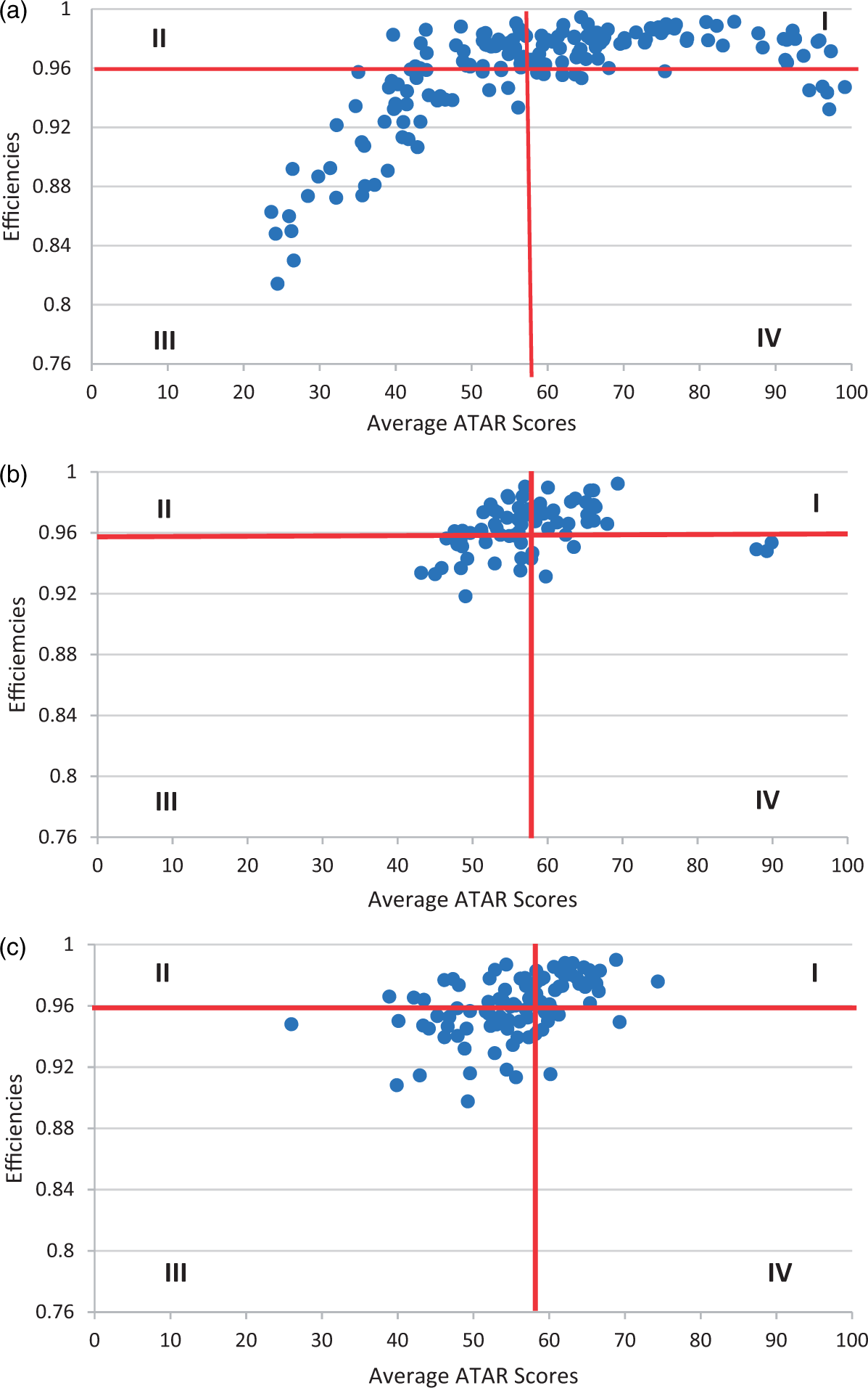

The efficiencies of the Metropolitan schools are further investigated as they have a very large spread of both ATAR scores and efficiencies. There are four districts in the Metropolitan area – Sydney, North Sydney, Western Sydney and South Western Sydney. For the Metropolitan region as a whole, the average efficiency is 0.958 and the average ATAR Score is 58.6. The percentage of schools in each of the four metropolitan districts is 21.0% in both the Sydney and North Sydney regions, 23.4% in the Western Sydney region and 34.7% in the South Western Region.

In Table 7, North Sydney has the highest ATAR score with the smallest standard error while the South-Western Sydney district has the lowest ATAR score and the smallest efficiency score. The difference between the district ATARs is significant except for between Western and South-Western Sydney. The difference between the average district efficiency for North Sydney and South Western Sydney is very large and significant (t-stat = 4.6) and between North Sydney and Sydney is also significant (t-stat = 2.4). The highest maximum average ATAR score is in the Western Sydney region (99.13) with the lowest maximum in the South-Western Sydney region (91.09) with a range of only 8.04. Another indication of the differences in the four regions is the minimum average ATAR scores – 56.15 for North Sydney and 26.0 for Sydney. This difference is much larger – 30.15.

Table 7.

Descriptive statistics for the ATAR and efficiency for the four metropolitan districts.

	Sydney		North Sydney		Western Sydney		South-Western Sydney
	ATAR	Efficiency	ATAR	Efficiency	ATAR	Efficiency	ATAR	Efficiency
Average	63.94	0.9614	73.55	0.9758	54.38	0.9541	49.19	0.9469
SD	18.62	0.0314	11.45	0.0153	16.92	0.0304	15.06	0.0433
Max	96.81	0.9944	97.08	0.9909	99.13	0.9903	91.09	0.9899
Min	26.00	0.8602	56.15	0.9319	26.46	0.8712	23.66	0.8149
N	35		35		39		58

Table 8 presents the efficiency matrix for the Metropolitan schools in each of the four quadrants by efficiency level and by district. Figure 4 illustrates the ranges for the efficiencies and median ATAR scores for each of the districts. Of the North Sydney schools, 80% are in Quadrant 1 compared with the Sydney region (57.1%) and South-Western Sydney (17.2%). Most concerning are schools in Quadrant III as these schools have below average educational achievement and also below average efficiency levels. North Sydney has the smallest percentage (2.8%) of its schools in Quadrant III but South-Western Sydney has almost half (44.8%) of its schools in Quadrant III.

Table 8.

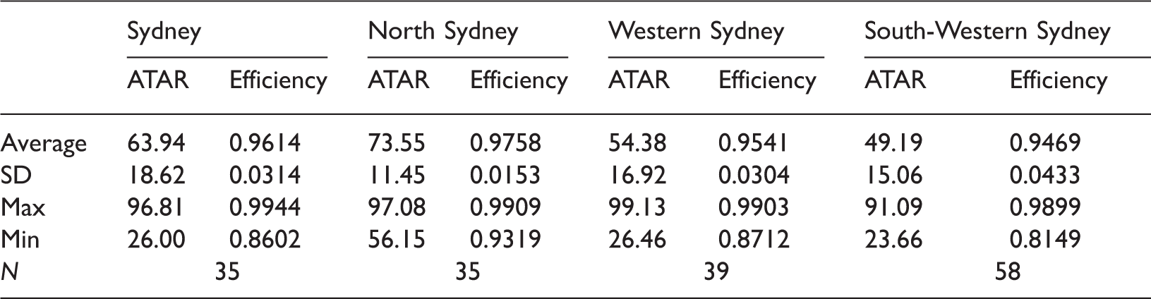
Efficiency matrix for the SFA Model for the metropolitan districts.

Quadrant II		Quadrant I
Sydney	5 (14.3%)	Sydney	20 (57.1%)
North Sydney	2 (5.7%)	North Sydney	28 (80.0%)
Western Sydney	12 (30.8%)	Western Sydney	11 (28.2%)
South-Western Sydney	21 (36.2%)	South-Western Sydney	10 (17.2%)
Total	40 (24.0%)	Total	69 (41.3%)
Quadrant III		Quadrant IV
Sydney	5 (14.3%)	Sydney	5 (14.3%)
North Sydney	1 (2.8%)	North Sydney	4 (11.4%)
Western Sydney	15 (38.5%)	Western Sydney	1 (2.6%)
South-Western Sydney	26 (44.8%)	South-Western Sydney	1 (1.7%)
Total	47 (28.1%)	Total	11 (6.6%)

Figure 4.

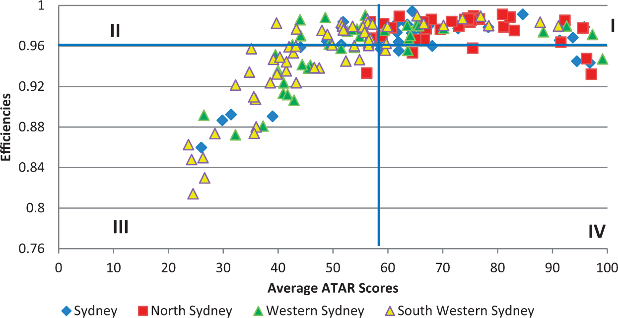
Average efficiencies for the Pitt/Lee HET Model for the four metropolitan districts.

Schools in Quadrant III are inefficient and ineffective with a number of schools performing at a very low level. Further work is needed to determine the specific characteristics of these schools, and what strategies can be implemented to raise both their efficiency and achievement levels. It is expected that the future addition of a FOEI indicator of family characteristics variable may help solve this problem.

Data limitations

Our current study has been constrained by the currently available school site data sets from the NSW Department of Education and Communities. Data on teacher year 12 Math/Science qualifications are of prime importance in model estimation, however, in NSW and across Australian schools generally, ‘teacher quality’ including teacher qualifications and student characteristic data are not systematically collected. This is in contrast to the United Kingdom where individual teacher variables and school student census variables are available. Further, as no information on class size data is available, it is not possible to include this variable in the current analyses.

Omitted variables bias occurs when a model is incorrectly specified and omits an independent variable that is correlated with both the dependent variable and one or more included independent variables. Such regression coefficients are then inconsistent. One variable that is missing is an SES variable. However, the model used has a number of variables that can serve as a proxy for SES. They include dummy variables for region, ratio of female students, the proportion of Indigenous students, the proportion of students attending school and the apparent average retention rate. We have also been able to include financial data in terms of teachers’ and other staff salaries per student which are rarely used.

Furthermore, endogeneity is not an issue as none of the independent variables depend on the ATAR results.

Conclusions

The NSW public secondary school system is currently a predominantly homogenous one that is mainly funded from State Government resources across a common curriculum. Our analysis has shown that there is a wide variation in the output (median ATAR) of these government schools. The efficiencies for the schools vary by median ATAR and by region and district. The most important variable in the analysis is the impact of prior learning achievement in Year 10 which is positive and significant. The outcome of the estimated efficiencies for each school highlights some problems which need addressing in the next stage of the authors’ research.

The authors plan to track the implementation and efficiency of new State policy directions with respect to the impact on schools’ outputs by continuing our SFA modelling using our updated base from 2011 onwards. In the next tranche of data modelling studies, we hope to include the FOEI (and or ICSEA) data as well as data from the NAPLAN tests in Years 7 and 9. This should increase our knowledge of the intake of students into the different schools as well as add family characteristics.